Modularity analysis of a health information platform from a network science perspective

KADIR HAS UNIVERSITY

GRADUATE SCHOOL OF SCIENCE AND ENGINEERING

MODULARITY ANALYSIS OF A HEALTH INFORMATION

PLATFORM FROM A NETWORK SCIENCE PERSPECTIVE

SEMİHA NUR ALAŞAN

S emi ha Nur AL AŞAN M. S . The sis 2015 S tudent’ s F ull Na me P h.D. (or M.S . or M.A .) The sis 20 11

MODULARITY ANALYSIS OF HEALTH INFORMATION

PLATFORM FROM A NETWORK SCIENCE PERSPECTIVE

SEMİHA NUR ALAŞAN

Submitted to the Graduate School of Science and Engineering In partial fulfillment of the requirements for the degree of

Master of Science In

Management Information Systems

KADIR HAS UNIVERSITY May, 2015

i

MODULARITY ANALYSIS OF HEALTH INFORMATION

PLATFORM FROM A NETWORK SCIENCE PERSPECTIVE

Abstract

As Barabási (2015) emphasizes that the very idea of communities goes back to the time people were born into communities and had to find their individuality. But today it is the other way around, that is, people are born individuals and have to find their communities. This research is aimed to better understand modularity measures for a health information platform. Such platform is an exemplary of its many kinds that are characterized as interactive, web-based information exchange platforms. These platforms draw attentions of academics due to its underlying complex systems behavior in various domains such as computer science, management science, sociology, and management information systems (MIS). We adopt a perspective of an emerging interdisciplinary field called network science that enables us to analyze modularity of a health information platform. The whole connection network normally has 2143 nodes and 5706 edges. In this research, since the modularity is examined, it is vague to integrate the sprinkled nodes over the giant component. Thus and so, the only giant component having 1652 nodes and 5146 edges is studied. This analysis is based on the modularity maximization algorithm, which Gephi uses as default, by assigning two different resolution values for the same data set to try which resolution value gives better results.

Keywords. Social Network Analysis, Modularity Analysis, Resolution Limits, Online Health Information Platform.

AP PE ND IX C

ii

AĞ BİLİMİ AÇISINDAN SAĞLIK BİLGİ PLATFORMUNDA MODÜL (MODULARITY) ANALİZİ

Özet

Barabási’nin (2015) de değindiği gibi eskiden insanlar bir topluluk içine doğup sonradan bireyselleşmeye çalışırken, günümüzde insanlar bireysel olarak doğup bir topluluk içine dahil olmaya çalışıyorlar. Bu çalışma, sağlık bilgi platformundaki modül (modularity) analizini yapıp gruplaşmayı modül kriterleri açısından incelemeyi amaçlıyor. Bu platform, bilgi alışverişinin sağlandığı interaktif web-tabanlı birçok platforma emsal teşkil ediyor. Bu platformlar, altında yatan karmaşık sistem davranışları sebebiyle akademisyenlerin dikkatini çekip bilgisayar bilimleri, yönetim bilimi, sosyoloji ve yönetim bilişim sistemleri ihtisaslarında incelemeye değer bulunuyor. Ağ bilimi olarak adlandırılan gelişmekte olan disiplinlerarası alanı bakış açısını benimseyerek sağlık bilgi platformunda modül analizi yaptık. Modül analizinde dev bileşenin etrafında yer alan bağımsız düğümleri incelemek anlamsız olacağından normalde 2143 düğüm (node) ve 5706 bağa (edge) sahip olan bağlantı ağının 1652 düğüm ve 5146 bağdan oluşan dev bileşeni (giant component) ele alındı. Bu analiz, aynı veriseti için iki farklı “resolution” değeri atanıp hangi “resolution” değerinin daha iyi sonuçlar verdiğini anlayabilmek için Gephi adlı yazılımın default olarak kullandığı “modül maksimizasyonu” (modularity maximization) algoritması baz alınarak yapıldı.

Anahtar kelimeler. Sosyal Ağ Analizi, Modül Analizi, “Resolution” limitleri, Online Sağlık Bilgi Platformu.

AP PE ND IX C

iii

Acknowledgements

First and foremost, I would like to show my gratitude to my thesis advisor Assoc. Prof. Dr. Mehmet N. AYDIN and his supportive colleague Asst. Prof. Dr. N. Ziya PERDAHÇI, who was always making our research meetings so much fun by making jokes and English-Turkish puns.

I place on record, my sincere gratefulness to my parents Ekrem ALAŞAN and Aynur ALAŞAN for supporting and encouraging me during my entire education life. I thank my dad for enjoying life under all circumstances and teaching it to me.

I would also like to thank my precious professors Assoc. Prof. Dr. Mehmet N. AYDIN, Prof. Dr. Hasan DAĞ, and Işıl TİRYAKİLER for always believing that I could overcome the challenges in life.

I would like to express my deepest appreciation to my fiancé Abdulkadir EROĞLU for cheering me up and his support.

In addition, I would like to thank all my classmates and friends Cansu Hazal MALKOÇ, Kübra ŞADOĞLU, Nurcan SOARES, Lacey WATSON, Emily CARDWELL, and Džordana KARINIAUSKAITE individually for their motivation and continuous support.

After all, I would like to show my courtesy to not just my great mentor but also my elder sister Yeşer BALMUMCU.

AP PE ND IX C APPENDIX B

iv Dedication page

v

Table of Contents

2.1. Basic Network Terminology ... 4

2.2. Evolution of Social Communities ... 6

2.3. Techniques to Identify Communities ... 7

2.4. Community Detection Applications ... 9

2.5. Modularity and Resolution Limit ... 11

Chapter 3 ... 14 Method ... 14 Chapter 4 ... 15 Results ... 15 Chapter 5 ... 25 Discussion ... 25 Chapter 6 ... 26 Conclusion ... 26 References ... 27 APPENDIX B AP PE ND IX C APPENDIX B

vi

List of Tables

Table 4.1. Overall list for modules with resolution 1 (of Version1) ... 17

Table 4.2. Overall list for modules with resolution .5 (of Version2) ... 18

Table 4.3. The number of visitors and physicians within Version1 ... 19

Table 4.4. The number of visitors and physicians within Version2 ... 20

Table 4.5. Distribution of sex within Version1 ... 21

Table 4.6. Distribution of sex within Version2 ... 21

Table 4.7. Distribution of hubs within Version1 in terms of role attribute (Visitor or Physician) of the nodes ... 23

Table 4.8. Distribution of hubs within Version2 in terms of role attribute (Visitor or Physician) of the nodes ... 24 AP

PE ND IX C

vii

List of Figures

Figure 2.1. Connectedness and Density Hypothesis (Barabási, 2015) ... 6 Figure 2.2. The Zachary Karate Club network & polar-coordinate dendogram the

network (Zachary, 1977) ... 7 Figure 2.3. The largest connected component of the network of network scientists (Porter, et al., 2009) ... 9 Figure 2.4. Communities in Belgium (Barabási, 2015) ... 10 Figure 4.1. The overall view of whole network showing visitors as red nodes, and

physicians as turquoise nodes with Force Atlas 2 layout in Gephi ... 15 Figure 4.2. The overall view of the giant component when the resolution is 1 (Version1) with Force Atlas 2 layout in Gephi ... 16 Figure 4.3. The overall view when the resolution is decreased to 0.5 (Version2) ... 17 AP

PE ND IX C

Chapter 1

Introduction

Network science is a novel still-in-progress transdisciplinary area which produces new methods, approaches, and techniques to make sense out of relationships between things including people and objects. Since the relationships in real life are not easy to understand, it is challenging to look at them in a network science perspective as well. The study of complex networks is yet to be mature and active field of scientific research inspired by the research of real-networks.

As a consequence of living in a technological era, we are surrounded by all kinds of technological means including smart phones, online network applications such as information platforms. Unlike previous generations, Y-generation and the newer one love sharing things they do even sometimes they mean nothing to other people. Younger generation even shares what they eat, tweet their complaints, or create some campaigns just creating a new hashtag. It is getting easier to be organized in social networks. Reaching a celebrity and send a message to her/him is not that hard by reason of globalization and social media. As small-world experiment proves that it takes at most 6 people to reach anyone in the small-world, even the president of US (Milgram, 1969).

Power of social networks is incontrovertible: People come together around a topic or belief using such platforms as a communication tool and may even hold a physical public demonstration. Therefore, social networks are not virtual, but in our real lives. We cannot think of a life isolated from social networks anymore.

Thanks to the growth of social media platforms, every person generates data and contributes to the big data. Any picture posted on Instagram, any sentence or even a word tweeted, or a video posted on Facebook are respected as data. Similarly, accepted friendship requests on Facebook, following relationships on Twitter and Instagram, or subscribers on YouTube are considered in terms of network science.

Without analyzing the raw data, data itself means nothing. The data is valuable when it is analyzed and transformed into information. To be able to evaluate information from the big data on social networks many approaches have been developed. Growing data necessitated the analysis to give a reasonable meaning which might be used in many different fields such as marketing to pinpoint the target market in advance. Since social networks are considered

2

as complex networks, the provided data can be studied from various points of view: Computer science, network science, or sociology. In our research, we are going to examine our data from a network perspective. However, to be able to analyze it better, the basic knowledge on sociology, statistics, social psychology and graph theory are required.

The difference between information networks and social networks is that information networks give us many important ideas about structure of the platform. To be able to call a network as an information network, there are criteria such as “Six Degrees of Separation” model conducted by Stanley Milgram and ensuring not only information pass but information exchange among people in the network. One of the most popular information networks is health social networks (e.g., HealthTap, WebMD). The increase in the Internet usage directed people to solve their problems online rather than spending time in queues in hospitals. Health social networks get more popular because of ease of reliable information access. “More than 700 of the US’ 5000 hospitals have a social media and social networking presence to enhance their ability to market services and communicate to stakeholders (Alaşan, et al., 2014).” There are lots of health social networks available such as healthtap.com, doktorumonline.net, doktorburada.com, and doktorsitesi.com. Basically, all websites mentioned above provide similar services: Visitors are able to access and ask questions about their illnesses to a physician or a visitor who has the same sickness or has had an experience about that sickness before.

We studied the data gathered from Doktorsitesi.com, which is one of the most popular online health platform in Turkey, in terms of modularity from a network science perspective. Doktorsitesi.com was established to meet both physicians and visitors having health problems. It is a platform that enables visitors to make appointments with physicians, help both physicians and visitors to ask questions to each other or send private messages. Asking questions is public, so that visible to all users. However, when sending private messages, only the sender and receiver of the message can see it. The platform has some rules to be able to send messages: It is only allowed to send messages between members (either a visitor or physician), if they are connected. Members get connected to each other when requested connection demands are accepted. From the network perspective, nodes represent members who are physicians or visitors, undirected links represent the ties that are edges between members. In this research, connection relationships among members are observed.

In this paper, it is aimed to analyze a health network by separating them into worthwhile modules which are more connected to each other in sense of degree.

3

Is it possible to group individuals in terms of their common interest and similar characteristics? Is there a specific way to separate a network into explicit communities? If so, depending on what could people aggregate in a network? Could groups in a network be estimated in advance? In this study, I try to answer such questions from a network perspective clarifying the works done before in Chapter 2, the methodology, the tools used, and steps taken to complete the whole analysis in Chapter 3, and showing the quantitative results as well as the overall graphs of my work in Chapter 4. In Chapter 5, the meaning of the results is depicted predicating the claims on the references. Ultimately, the limitations of the study and further work based on this research are revealed in Chapter 6.

4

Chapter 2

Research Background

From an abstract view, a network can be represented as a graph in mathematical sense. Among various fields, a network has so many different meanings. The United States National Research Council defines network science as “the study of network representations of physical, biological, and social phenomena leading to predictive models of these phenomena” (Council, 2006). Network science is such a wide field that every disciplinary has its own definition for it. In sociology, for example, each node of a network represents an agent, and a pair of nodes is connected to each other by an edge or link. Binary pairwise connections, which are the simplest types of edges, are called ties. In addition, edges can be assigned to a direction considering positive or negative weights to observe various interactions among nodes.

Networks might be categorized depending on the relationship between nodes: An undirected

network is the one in which edges have no orientation and there is symmetry between edges.

For example the edge (Node A to Node B) is identical to the edge (Node B to Node A. Basically, the edges in such networks have no direction. The maximum number of edges in such networks without a self-loop is calculated by (n*(n - 1))/2, n is the number of nodes in the network. Becoming friends on Facebook, road maps, airline route maps, electrical circuits, and computer networks are considered as undirected networks.

Directed networks on the other hand, a set of nodes that are connected together, where all the

edges are directed from one node to another, there is no symmetry between edges. A directed network is also called a digraph. Exceptionally, a node can have an edge to itself, so an edge Node A to Node A is valid. A financial network is an instance of a directed network; transactions are edges, while currency or stocks are nodes. Similarly, the World Wide Web is recognized as directed network, calling web pages as nodes (vertexes) and hyperlinks connecting web pages are edges (links). Correspondingly, a telephone network which consists of people as nodes, and placed calls made by people as edges is defined as a directed network.

Networks may also be grouped as weighted or unweighted in terms of number of edges between nodes. If there is only one edge between nodes, it is simply called a unweighted

5

network. When there is more than one edge among two nodes, then the network is called a weighted network. A connection network such as friendship or membership is an unweighted

network, whereas a text message network between two people is considered as weighted because of the number of messages received and sent.

In the study of networks, the degree of a node in a network is the number of connections it has to other nodes and the degree distribution is the probability distribution of these degrees over the whole network (Albert & Barabási, 2002).

Average path length is a concept in network science which is defined as the average number

of steps along the shortest paths for all possible pairs of network nodes. It is a measure of the efficiency of information or mass transport on a network (Albert & Barabási, 2002). The shorter the path length is, the easier for information to transport throughout the whole network.

In a mesoscopic structure, a group of nodes that are relatively intensively connected to each other but infrequently connected to other dense groups in the network is called a community (Fortunato, 2010).

Albert-László Barabási came up with the H2, which stands for Hypothesis 2: Connectedness

and Density Hypothesis, to be able to define communities. Depending on H2, “A community

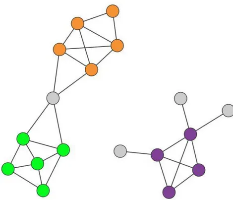
is a locally dense connected subgraph in a network. In other words, all members of a community must be reached through other members of the same community (connectedness). At the same time we expect that nodes that belong to a community have a higher probability to link to the other members of that community than to nodes that do not belong to the same community (density). While this hypothesis considerably narrows what would be considered a community, it does not uniquely define it. Shown in Fig. 2.1 below, H2 relies on two different hypotheses: Connectedness hypothesis declare that each community corresponds to a connected subgraph, like the subgraphs formed by the orange, green or the purple nodes. Consequently, if a network consists of two isolated components, each community is limited to only one component. The hypothesis also implies that on the same component a community cannot consist of two subgraphs that do not have a link to each other. Consequently, the orange and the green nodes form separate communities. Density hypothesis on the other hand, claims nodes in a community are more likely to connect to other members of the same community than to nodes in other communities. The orange, the green and the purple nodes satisfy this expectation (Barabási, 2015).”

6

Figure 2.1: Connectedness and Density Hypothesis (Barabási, 2015) 2.2. Evolution of Social Communities

Studies in the history prove the existence of social communities in a variety of networks. Human grouping patterns have been investigated for a long time especially in sociology (Freeman, 2004) and social anthropology (Kottak, 1991): Stuart Rice clustered data manually to ascertain political groups in the 1920s (Rice, 1927), and George Humans clarified the importance of rearranging the rows and columns of data matrices in 1950 (Homans, 1950). In 1955, Robert Weiss and Eugene Jacobson practiced the first community structure analysis (Weiss & Jacobson, 1955).

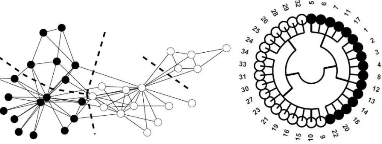
In regards to community detection, sociologist Wayne Zachary’s Karate Club example is considered as a milestone and also a benchmark to detect groups in networks. In this study, an internal dispute led to the schism of a karate club into two smaller clubs (Zachary, 1977). When the club split in two, its members chose preferentially to be in the one with most of their friends. Zachary comprehended that he might anticipate the split in advance.

In Fig. 2.2 below, two communities in Karate Club network are shown with two different visualization techniques. “The Zachary Karate Club network has a natural hierarchy of decompositions: a coarse pair of communities that correspond precisely to the observed membership split, and a finer partition into four communities. In larger networks, for which algorithmic methods of investigation are especially important, the presence of multiple such

7

partitions indicates mesoscopic network structures at different mesoscopic resolution levels. At each level, one can easily compare the set of communities with identifying characteristics of the nodes (e.g., the post-split Karate Club memberships) by drawing a pie chart for each community, indicating the composition of node characteristics in that community (Porter, et al., 2009).”

Figure 2.2: The Zachary Karate Club network (on the left) & polar-coordinate dendogram the network (on the right) (Zachary, 1977)

In Fig. 2.2 on the left side, the Zachary Karate Club network is visualized using the Fruchterman-Reingold method (Fruchterman & Reingold, 1991). Nodes are colored black or white depending on their later club affiliation after a disagreement prompted the organization’s breakup. On the right side, polar-coordinate dendrogram representing the results of applying the community-detection algorithm to the network is shown. One may realize the obvious split of the network into two groups which are identical to the observed membership of the new clubs (Porter, et al., 2009).

Since sociologists needed powerful mathematical tools and data analysis tools to detect communities, physicians took action to create such algorithms. An important step was taken in 2002, when Michelle Girvan and Mark Newman brought graph-partitioning problems to the broader attention of the statistical physics and mathematics communities (Girvan & Newman, 2002).

2.3. Techniques to Identify Communities

The idea of organizing data by separating them based on common features goes long way back in the history (Slater, 2008). Especially physicians put so much effort on that issue in terms of generating algorithms, while sociologists tried to examine that affair in a way of understanding domains and basic characteristics of the networks.

8 2.3.1. Traditional Clustering Techniques

The original computational studies to detect clusters of similar objects are based on statistics and data mining (Porter, et al., 2009). Important methods include partitional clustering

techniques such as k-means clustering, neural network clustering techniques such as

self-organizing maps, and multi-dimensional scaling (MDS) techniques such as singular value decomposition (SVD) and principal component analysis (PCA) (Gan, et al., 2007).

The other outstanding classical techniques are hierarchical clustering algorithms such as the

linkage clustering methods. In addition, there are divisive techniques, where one starts with

the full graph and separates it into several groups to find communities (Fortunato, 2010).

2.3.2. Centrality-Based Community Detection

Michelle Girvan and Mark Newman brought a new view to the sociological notion of betweenness centrality. They caught greater attention in mathematics and statistical physics when they invented a community-finding algorithm based on centrality, which basically gives an idea about how central and important nodes in a whole network. “An edge has high betweenness if it lies on a large number of paths between vertices. If one starts at a node and wants to go to some other node in the network, it is clear that some edges will experience a lot more traffic than others” (Porter, et al., 2009).

2.3.3. Modularity Optimization

One of the most popular quality functions is modularity that tries to understand how well a given portion of a network separates into its communities. Quality functions such as modularity maintains explicit statistical criteria to count the total strength of connections within communities versus those between communities (Newman & Girvan, 2003).

“Modularity is a scaled assortativity measure based on whether high-strength edges are more or less likely to be adjacent to other high-strength edges. Because communities are supposed to have high edge density relative to other parts of the graph, a high-modularity partition tends to have high edge-strength assortativity by construction” (Porter, et al., 2009).

2.3.4. The Kernighan-Lin Algorithm

It is an algorithm nominated by Brian Kernighan and Shen Lin (KL) to find out how to split electric circuits into boards so that the nodes in different boards can be linked to each other following the most efficient path in terms of length (Kernighan & Lin, 1970).

2.3.5. k-Clique Percolation

The method of k-clique percolation is based on the concept of a k-clique, which is a complete subgraph of k nodes that are connected with all k*(k − 1)/2 possible links (Palla, 2005). The

9

method depends on the examination of communities whether they have small cliques that share many of their nodes with other cliques in the same community.

2.3.6. Spectral Partitioning

The method of spectral partitioning emerged for parallel computation. In traditional spectral partitioning, network properties are related to the spectrum of the graph’s Laplacian matrix L, examining the Kronecker delta (Pothen, et al., 1990). Basically, the method starts by separating a network into two components. One then applies two-group partitioning recursively to the smaller networks one obtains as long as the result satisfies to do so (Richardson, et al., 2008).

2.4. Community Detection Applications 2.4.1. Scientific Collaboration Networks

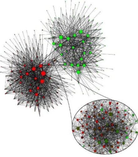
In the literature, a well-known co-authorship network, which has scientists linked to papers that they authored or co-authored, has been investigated as an indicator of community-detection. The largest connected component (379 nodes) of the co-authorship network with 1589 scientists as nodes is shown in the Fig. 2.3, using a Kamada-Kawaii visualization, is colored according to its community assignment using the leading-eigenvector spectral method (Newman, 2006).

10 2.4.2. Communities in Belgium

The Belgium appears to be the model of a bicultural society: 59% of its citizens are Flemish, speaking Dutch and 40% are Walloons who speak French. Vincent Blondel and his students find an answer for how Belgium fostered the peaceful coexistence of these two ethnic groups since 1830. In 2007, Blondel and his students started to examine the public from the mobile call network, placing individuals next to whom they regularly called on their mobile phone (Blondel, et al., 2008). The algorithm reported that Belgium’s social network is broken into two large clusters of communities and that individuals in one of these clusters rarely talk with individuals from the other cluster, shown in Fig. 2.4 below. “The origin of this separation became obvious once they assigned to each node the language spoken by each individual, learning that one cluster consisted almost exclusively of French speakers and the other collected the Dutch speakers (Barabási, 2015)”.

11 2.4.3. Online Social Networks

Social networking sites are prevalent part of everyday life. “They allow users to construct a public or semi-public online profile within a bounded system, articulate a list of other users (called “friends”) with whom they share a connection, and view and traverse their network of connections” (Traag & Bruggeman, 2009). Social network web sites such as Facebook, LinkedIn, MySpace, and hundreds of others have collectively attracted over one billion users since they have been established. People have easily accepted social network sites into their daily lives, for many different purposes: to communicate with friends, send e-mails, solicit opinions or votes, organize events, spread ideas, find jobs, and so on.

The appearance of social network web sites has enabled scientists and sociologists to reach quantitative social and demographic data (Boyd & Ellison, 2007).

This has obviously been a big deal for social scientists, but numerous mathematicians, computer scientists, physicists, and more have also had a lot of fun with this new wealth of data, which is called big data. Big data is everywhere, waiting for data scientists to analyze it and turn it into valuable information.

2.4.4. Biological Networks

Communities have a significant role to perceive how particular biological functions are concealed in cellular networks and to understand human diseases. “Ravasz and collaborators made the first attempt to systematically identify such modules in metabolic networks. They did so by building an algorithm to identify groups of molecules that form locally dense communities (Barabási, 2015)”. It is proved that proteins which are involved in the same disease tend to interact with each other (Goh, et al., 2007). In this fashion, since health is the point in the question, community detection becomes a more important issue.

2.5. Modularity and Resolution Limit

The definition of modularity is stated as the following expression in Barabási’s book: “In a randomly wired network the connection pattern between the nodes is expected to be uniform, independent of the network's degree distribution. Consequently these networks are not expected to display systematic local density fluctuations that we could interpret as communities. This expectation inspired the third hypothesis of community organization: H3:

Random Hypothesis is explained as randomly wired networks lack an inherent community

structure. This hypothesis has some actionable consequences: By comparing the link density of a community with the link density obtained for the same group of nodes for a randomly

12

rewired network, we could decide if the original community corresponds to a dense subgraph, or its connectivity pattern emerged by chance.

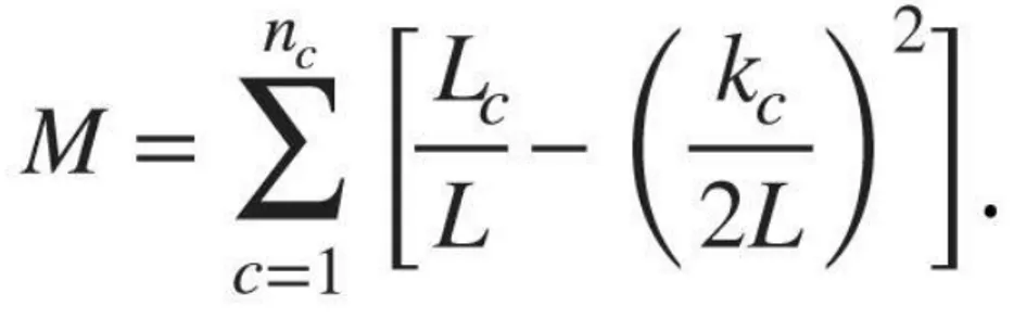
Consider a network with N nodes and L links and a partition into nc communities, each community having Nc nodes connected to each other by Lc links, where c=1,...,nc, and kc is the total degree of the nodes in this community. If Lc is larger than the expected number of links between the nc nodes given the network’s degree sequence (Barabási, 2015)”. The formula to calculate modularity is shown below in Fig 2.5:

Figure 2.5: Modularity formula (Barabási, 2015)

To better understand the modularity, some key properties are explained as well:

Modularity value can be between -1 and 1. When the modularity value is higher, the partition of the network is better (Barabási, 2015), meaning it suits better with real life and partition becomes domain-specific. If all nodes are assigned to the same community, modularity value becomes zero.

Barabási has also mentioned about H4: Maximal Modularity Hypothesis, which has a definition as follows: For a given network the partition with maximum modularity corresponds to the optimal community structure. “The maximum modularity hypothesis is the starting point of several community detection algorithms, each seeking the partition with the largest modularity. In principle we could identify the best partition by checking M for all possible partitions, selecting the one for which M is largest. Given, however, the exceptionally large number of partitions, this brute-force approach is computationally not feasible (Barabási, 2015)”.

The Greedy algorithm introduced by Mark E. J. Newman was the first modularity maximization approach. What it basically affirms is considering each node as a community at the beginning, calculating modularity one by one for the neighbor nodes, and assigning the nodes to the communities where modularity value is higher (Newman, 2004).

Modularity maximization forces small communities into larger ones (Fortunato & Barthélemy, 2007). “Modularity maximization cannot detect communities that are smaller

13

than the resolution limit. For example, for the WWW sample with L=1,497,134 modularity maximization will have difficulties resolving communities with total degree kc is (approximately) smaller than 1,730. Real networks contain numerous small communities. Given the resolution limit, these small communities are systematically forced into larger communities, offering a misleading characterization of the underlying community structure (Barabási, 2015)”.

14

Chapter 3

Method

The data set is received from the well-known Turkish online health platform Doktorsitesi members, which are either physicians or patients as nodes, and the connection between them as edges. All records of established connections over the 3-month period from October to December 2012 are examined. For each connection, all information regarding the transaction that resulted in a connection is gathered. Description of the network data and visual analysis of network diagrams and overall views are generated with Gephi (Bastian, et al., 2009), which is an open-source and free visualization and exploration software for social network analysis. Gephi is an ongoing platform created by the French. In addition, Microsoft Excel is used to sort the data and create tables.

It is modeled the giant component of the whole network, which normally has 2143 nodes and 5706 edges. In this study, since the modularity is probed, it makes no sense to integrate the sprinkled nodes over the giant component. Thus and so, the only giant component having 1652 nodes and 5146 edges is examined.

Although the connection network examined as a graph of directed edges, it is considered as an undirected ones because of the modularity algorithm generated by Gephi is applicable to undirected ones.

The connection network is represented in general in Table 1 and Table 2 showing the basic statistics of the connection request network as well as the modularity class IDs depending on the resolution. Version 1 has 20 individual modules, while Version 2 possesses 40 modules. The difference is because of from how close the network is examined, which is simply the resolution value selected. Nodes are called “Physician” and “Visitor”, which are actually patients, in the tables. It is have connections between Physician-Physician, Visitor-Visitor or Physician-Visitor in the platform examined.

Two key measures, node degrees and path length, maintain effective but finite insights about the structure of the connection network. The degree of a node in a network is the number of connections or edges the node has to other nodes. In such a way, average degree shows the degree of the most of the nodes in the network. “Path length measures the distance between nodes in terms of number of connections in the network examined. Thus, it simply shows how far apart people (Physicians and Visitors) are” (Aydın & Perdahçı, 2014).

Following tables show in detail the distribution of sex and hubs that are considered as the most important people in a network in terms of information exchange.

15

Chapter 4

Results

Gephi cannot take the attributes of nodes into account when modularity analysis is performed. It only considers degree of nodes and edges. Hence, the attributes of the nodes are not taking into account in terms of calculation. However, it is still possible to estimate the some basics of the connection network since the domain is known.

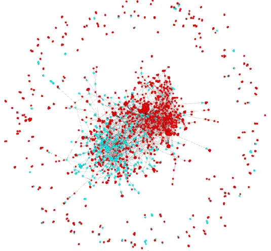
Figure 4.1: The overall view of whole network showing visitors as red nodes, and physicians as turquoise nodes with Force Atlas 2 layout in Gephi

The network examined shown in Fig 4.1 has 2143 nodes and 5706 edges as total. 74.48% of whole network is visitors, while physicians form the 25.52% of the connection network. Since we focus on the tie network, it makes more sense to work on the giant network instead of the whole network. The giant component, which has 1652 nodes and 5146 edges, is examined with different resolution values in order to define modules.

16

The giant component corresponds to the 77.09% of the whole network. There are 1224 visitors, which are most probably patients, 428 physicians in the giant component. 910 of whole visitors are female, while only 128 of physicians are female. On the other hand, 314 of visitors are males whereas there are 300 male physicians in the giant component. Obviously, the connection network of Doktorsitesi is a female dominant network matching to the 62.83% of the giant component. Over and above, the 74.1% of the giant component is visitors.

When the resolution is 1, which is the default value provided by Gephi referencing the Greedy algorithm, which is considered as the first modularity maximization approach and introduced by Mark E. J. Newman (Blondel, et al., 2008), 20 modules are provided. 20 modules in one are abbreviated to “Version 2” for the following work.

As the resolution is decreased, the number of modules increases. So that, when the resolution is taken as 0.5, 40 modules are provided in the same network. 40-mod version is henceforth called simply “Version2”.

It is worth to categorize all these modules depending on their attributes such as the role (Physician-dominant modules or Patient-dominant modules), sex (Female-dominant modules or Male-dominant modules), and the importance of hubs, that are the nodes whose degree is 16 or higher.

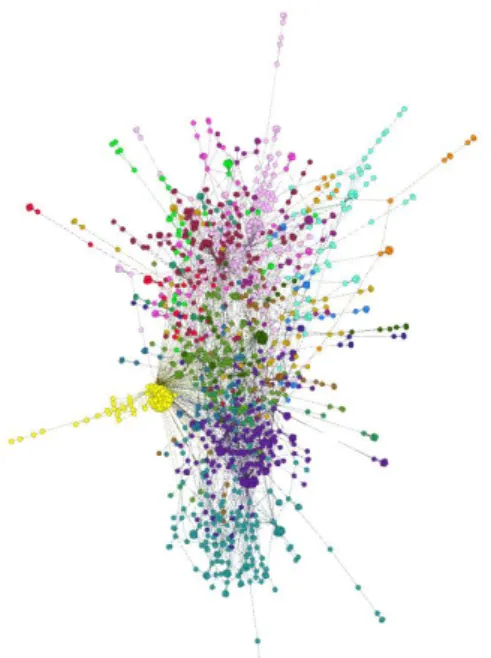
Figure 4.2: The overall view of the giant component when the resolution is 1 (Version1) with Force Atlas 2 layout in Gephi

17

Figure 4.3: The overall view when the resolution is decreased to 0.5 (Version2)

Colors on Figure 4.2 and Figure 4.3 vary depending on the modules. On the first graph there are 20 modules, while the second one constitutes 40 modules. As can be seen clearly, the number of modules increases as the resolution decreases.

Modularity

Class ID Nodes Edges

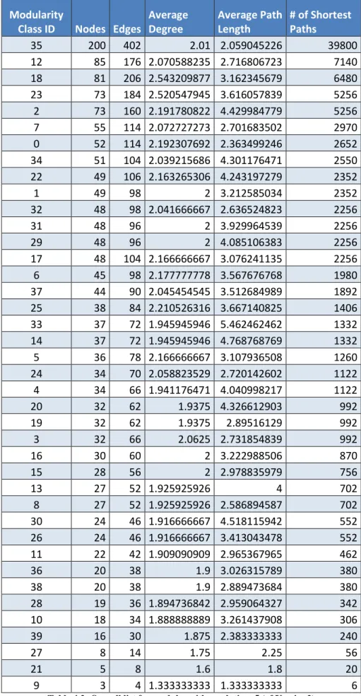
Average Degree Average Path Length # of Shortest Paths 3 221 650 2.94117647 3.569477581 48620 9 208 418 2.00961538 2.160628019 43056 7 185 478 2.58378378 4.486016451 34040 14 181 418 2.30939227 3.651074279 32580 12 141 321 2.27659574 4.036372847 19740 5 129 308 2.3875969 3.803657946 16512 13 73 150 2.05479452 4.880898021 5256 11 58 118 2.03448276 2.948578342 3306 19 54 110 2.03703704 5.456324249 2862 6 53 116 2.18867925 3.277213353 2756 17 48 94 1.95833333 4.436170213 2256 18 46 90 1.95652174 4.833816425 2070 4 45 90 2 3.383838384 1980 10 43 88 2.04651163 3.508305648 1806 2 41 80 1.95121951 3.782926829 1640 1 33 64 1.93939394 3.625 1056 8 30 58 1.93333333 4.972413793 870 0 24 46 1.91666667 3.413043478 552 16 20 38 1.9 3.157894737 380 15 19 36 1.89473684 4.116959064 342

18

Modularity

Class ID Nodes Edges

Average Degree Average Path Length # of Shortest Paths 35 200 402 2.01 2.059045226 39800 12 85 176 2.070588235 2.716806723 7140 18 81 206 2.543209877 3.162345679 6480 23 73 184 2.520547945 3.616057839 5256 2 73 160 2.191780822 4.429984779 5256 7 55 114 2.072727273 2.701683502 2970 0 52 114 2.192307692 2.363499246 2652 34 51 104 2.039215686 4.301176471 2550 22 49 106 2.163265306 4.243197279 2352 1 49 98 2 3.212585034 2352 32 48 98 2.041666667 2.636524823 2256 31 48 96 2 3.929964539 2256 29 48 96 2 4.085106383 2256 17 48 104 2.166666667 3.076241135 2256 6 45 98 2.177777778 3.567676768 1980 37 44 90 2.045454545 3.512684989 1892 25 38 84 2.210526316 3.667140825 1406 33 37 72 1.945945946 5.462462462 1332 14 37 72 1.945945946 4.768768769 1332 5 36 78 2.166666667 3.107936508 1260 24 34 70 2.058823529 2.720142602 1122 4 34 66 1.941176471 4.040998217 1122 20 32 62 1.9375 4.326612903 992 19 32 62 1.9375 2.89516129 992 3 32 66 2.0625 2.731854839 992 16 30 60 2 3.222988506 870 15 28 56 2 2.978835979 756 13 27 52 1.925925926 4 702 8 27 52 1.925925926 2.586894587 702 30 24 46 1.916666667 4.518115942 552 26 24 46 1.916666667 3.413043478 552 11 22 42 1.909090909 2.965367965 462 36 20 38 1.9 3.026315789 380 38 20 38 1.9 2.889473684 380 28 19 36 1.894736842 2.959064327 342 10 18 34 1.888888889 3.261437908 306 39 16 30 1.875 2.383333333 240 27 8 14 1.75 2.25 56 21 5 8 1.6 1.8 20 9 3 4 1.333333333 1.333333333 6

19 In both versions, average degree is similar, which is 2.

As shown in Table 4.1, the minimum degree value in Version 1 is 1.9, whereas the maximum one is 2.94. In Table 4.2, the lowest degree value is 1.33, while the highest degree value is 2.01.

The minimum average path length of Version1 is 2.16, whereas the minimum average path length of Version2 is 1.33. Version1 is more efficient in terms of information transport on the network (Albert & Barabási, 2002). The maximum average path length of Version1 is 5.45, while the maximum average path length of Version2 is 5.46.

The maximum number of shortest paths of Version1 is 48620, while the maximum number of shortest paths of Version2 is 39800. The minimum number of shortest paths of Version1 is 342, while the minimum number of shortest paths of Version2 is 6. Most real networks have a very short average path length leading to the concept of a “small world” phenomena (Milgram, 1969), where everyone is connected to everyone else through a very short path. Gephi assigns random modularity class IDs every time the modularity algorithm is executed. So it gets more challenging to follow the changes between Version1 and Version2.

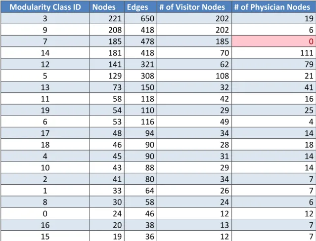
Modularity Class ID Nodes Edges # of Visitor Nodes # of Physician Nodes

3 221 650 202 19 9 208 418 202 6 7 185 478 185 0 14 181 418 70 111 12 141 321 62 79 5 129 308 108 21 13 73 150 32 41 11 58 118 42 16 19 54 110 29 25 6 53 116 49 4 17 48 94 34 14 18 46 90 28 18 4 45 90 31 14 10 43 88 29 14 2 41 80 34 7 1 33 64 26 7 8 30 58 24 6 0 24 46 12 12 16 20 38 13 7 15 19 36 12 7

20

Modularity Class ID Nodes Edges # of Visitor Nodes # of Physician Nodes

35 200 402 195 5 12 85 176 26 59 18 81 206 80 1 23 73 184 73 0 2 73 160 53 20 7 55 114 23 32 0 52 114 51 1 34 51 104 21 30 22 49 106 49 0 1 49 98 41 8 32 48 98 36 12 31 48 96 30 18 29 48 96 31 17 17 48 104 20 28 6 45 98 35 10 37 44 90 38 6 25 38 84 37 1 33 37 72 25 12 14 37 72 29 8 5 36 78 36 0 24 34 70 32 2 4 34 66 20 14 20 32 62 16 16 19 32 62 32 0 3 32 66 7 25 16 30 60 16 14 15 28 56 18 10 13 27 52 17 10 8 27 52 16 11 30 24 46 13 11 26 24 46 12 12 11 22 42 17 5 36 20 38 14 6 38 20 38 15 5 28 19 36 15 4 10 18 34 11 7 39 16 30 12 4 27 8 14 5 3 21 5 8 5 0 9 3 4 2 1

Table 4.4: The number of visitors and physicians within Version2

When the modules are named depending on node roles as visitor or physician modularity, surprisingly the number of visitor nodes exceeds the number of physician nodes in most of

21

the modules. To be more precise, visitors create more modules among themselves than the physicians do. There are even some modules that have no physicians at all. By analyzing the Version1 and Version2, it can explicitly be said that the number of patient nodes are more than the number of physician nodes in most of the modules. In addition, mod ID 7 in Version1 contains only visitors. Similarly, mod IDs 23, 22, 5, 19, and 21 in Version2 have no physicians.

Modularity

Class ID Nodes Edges

# of Female Visitors # of Male Visitors # of Female Physicians # of Male Physicians 3 221 650 163 39 16 3 9 208 418 139 63 4 2 7 185 478 142 43 0 0 14 181 418 42 28 17 94 12 141 321 47 15 20 59 5 129 308 98 10 3 18 13 73 150 23 9 18 23 11 58 118 34 8 9 7 19 54 110 16 13 15 10 6 53 116 39 10 1 3 17 48 94 17 17 2 12 18 46 90 15 13 2 16 4 45 90 16 15 1 13 10 43 88 18 11 2 12 2 41 80 27 7 2 5 1 33 64 20 6 3 4 8 30 58 19 5 2 4 0 24 46 10 2 7 5 16 20 38 13 0 3 4 15 19 36 12 0 1 6

Table 4.5: Distribution of sex within Version1

Modularity

Class ID Nodes Edges

# of Female Visitors # of Male Visitors # of Female Physicians # of Male Physicians 35 200 402 133 62 3 2 12 85 176 14 12 3 56 18 81 206 68 12 1 0 23 73 184 58 15 0 0 2 73 160 39 14 16 4 7 55 114 20 3 10 22 0 52 114 46 5 0 1 34 51 104 15 6 2 28 22 49 106 36 13 0 0

22 1 49 98 37 4 0 8 32 48 98 29 7 7 5 31 48 96 8 22 2 16 29 48 96 17 14 5 12 17 48 104 14 6 4 24 6 45 98 34 1 2 8 37 44 90 31 7 5 1 25 38 84 24 13 1 0 33 37 72 16 9 2 10 14 37 72 23 6 1 7 5 36 78 27 9 0 0 24 34 70 27 5 0 2 4 34 66 12 8 12 2 20 32 62 9 7 8 8 19 32 62 22 10 0 0 3 32 66 6 1 11 14 16 30 60 12 4 0 14 15 28 56 12 6 9 1 13 27 52 15 2 4 6 8 27 52 10 6 1 10 30 24 46 13 0 2 9 26 24 46 10 2 7 5 11 22 42 13 4 1 4 36 20 38 7 7 1 5 38 20 38 12 3 1 4 28 19 36 15 0 2 2 10 18 34 8 3 3 4 39 16 30 10 2 1 3 27 8 14 2 3 0 3 21 5 8 4 1 0 0 9 3 4 2 0 1 0

Table 4.6: Distribution of sex within Version2

There are no modules which do not have any female visitors. Female visitors have dominance over both physicians and male visitors regardless of the number of modules when the resolution is changed. There are even 2 modules (mod ID 16 and 15 in Version1) which have no male visitors. Similarly, 3 modules (mod ID 30, 28, and 9) in Version2 have no male visitors. Exceptionally, mod 31 in Version2 has more male visitors than female ones.

Unlike the dominance of female visitors, male physicians exceed the female physicians in modules for both cases.

Hubs are heavily linked nodes which tend to quickly accumulate more links. Hubs by definition exhibit high betweenness centrality which allows short paths to exist between

23

nodes (Albert & Barabási, 2002). In our research, we consider that hubs are the nodes whose degree is 16 or higher. Modularity Class ID Nodes Edges # of Hubs # of Visitor Hubs # of Physician Hubs 3 221 650 20 20 0 9 208 418 1 0 1 7 185 478 17 17 0 14 181 418 7 5 2 12 141 321 7 3 4 5 129 308 13 4 9 13 73 150 4 0 4 11 58 118 5 3 2 19 54 110 4 1 3 6 53 116 5 5 0 17 48 94 3 0 3 18 46 90 4 1 3 4 45 90 2 1 1 10 43 88 4 3 1 2 41 80 2 1 1 1 33 64 2 0 2 8 30 58 2 1 1 0 24 46 3 1 2 16 20 38 1 0 1 15 19 36 2 0 2

Table 4.7: Distribution of hubs within Version1 in terms of role attribute (Visitor or Physician) of the nodes

Modularity Class

ID Nodes Edges

# of

Hubs # of Visitor Hubs

# of Physician Hubs 35 200 402 1 0 1 12 85 176 1 1 0 18 81 206 8 8 0 23 73 184 8 8 0 2 73 160 3 3 0 7 55 114 1 1 0 0 52 114 5 5 0 34 51 104 3 2 1 22 49 106 4 4 0 1 49 98 2 0 2 32 48 98 4 3 1 31 48 96 2 1 1 29 48 96 4 0 4 17 48 104 4 2 2

24 6 45 98 6 1 5 37 44 90 5 3 2 25 38 84 4 4 0 33 37 72 4 1 3 14 37 72 2 0 2 5 36 78 4 4 0 24 34 70 2 2 0 4 34 66 4 1 3 20 32 62 2 1 1 19 32 62 2 2 0 3 32 66 1 0 1 16 30 60 1 1 0 15 28 56 2 2 0 13 27 52 1 0 1 8 27 52 2 1 1 30 24 46 2 0 2 26 24 46 3 1 2 11 22 42 2 2 0 36 20 38 2 0 2 38 20 38 2 1 1 28 19 36 2 0 2 10 18 34 2 1 1 39 16 30 1 0 1 27 8 14 0 0 0 21 5 8 0 0 0 9 3 4 0 0 0

Table 4.8: Distribution of hubs within Version2 in terms of role attribute (Visitor or Physician) of the nodes Undoubtedly, visitor hubs are much more than physician ones in both versions showing in Fig 4.7 and 4.8. In addition, a clear majority of the hubs are female.

In Version1, the correlation between the number of visitor nodes and the number of physician nodes is -0.01856. The correlation between the number of all nodes and the number of hubs with outliers is 0.705709. The correlation between average degree values and average path length values is -0.02002.

In Version2, the correlation between the number of visitor nodes and the number of physician nodes is -0.15609462. The correlation between the number of all nodes and the number of hubs with outliers (outliers are the modules # 35, 27, 21, and 9.) is 0.245828961. The correlation between the number of all nodes and the number of hubs excluding outliers is 0.519172957. The correlation between average degree values and average path length values is 0.330753355.

25

Chapter 5

Discussion

From the network science perspective, firstly interpreting the network basics meets requires both network science-related theoretical accounts (if they are mature enough) and domain knowledge, which frames the context of platform use. These two aspects (theoretical underpinnings and domain knowledge) challenge us to discuss the results with complete validation. Nevertheless, we attempt to raise some interesting points along with results and aim to bring out some future research questions.

Having roughly 3 as a value for the average degree of giant component might be simply depicted as the presence of many nodes which have at least 3 degree values (they can be in-degree or out-in-degree) in the connection network. Additionally, the value of the average path length is 4 means that the distance between regarding number of connections in the network is generally 4.

When focusing on Version 1 and Version 2, the highest and lowest degree values are both higher in Version 1. Apparently, Version 1 meets the criteria better than Version 2 in terms of degree for information transport (Albert & Barabási, 2002). On the other hand, average path length values in Version 1 are higher than Version 2. It is a proof that Version 2 is more reliable in terms of shortest path length as mentioned in the literature: Most real networks have a very short average path length leading to the concept of the “small world” phenomena, where everyone is connected to everyone else through a very short path (Milgram, 1969). So, one cannot 100% surely advocate that modularity analysis is better when the resolution value is considered 1 or 0.5. In order to decide which version is better, the other parameters of the network should be examined and the domain of the network should be understood so well. Still, one could argue that Version 1 should be selected when compartmentalizing the whole network.

It is also found that there are 2 modules (mod ID 16 and 15 in Version1) which have no male visitors. Those modules are more likely to be communities that are related to gynecological diseases.

26

Chapter 6

Conclusion

Taking everything into consideration, it could conveniently be said that network science helps researcher and practitioners to better understand complex behavior underlying web platforms. This research is a step towards to illustrate this understanding with a modularity analysis of an online health information platform, which deserves to be analyzed further as a prospective online social network. The attempt in this research was to structure the connection network of the health platform into modules using two different resolution values, and try to group members in the network depending on their common interest and similar characteristics. For modularity analysis we used an edge attribute (degrees) and take into account nodes attributes (gender: male, female and roles: physicians and visitors) to characterize the identifiers modules and make sense what underlies the formation of these modules. While identifying the modules, we were limited by Gephi as a tool in many aspects. It is more viable to keep the resolution value as default, which is 1, in Gephi. However, one cannot defend that resolution value must be left default unless having relevant results and evidence.

This research is restricted in many ways: The software used to analyze the connection network is limited in terms of modularity analysis. Hence, the network separated into modules only considering the degree values of nodes, not the attributes of nodes. In addition, since the areas of expertise of the physicians are not known, the domain of the health network was not enough to best describe the modules.

For the future work, with a larger and recent data set the same modularity analysis could be generated using a better software tool which takes attributes of the nodes into account as well. Moreover, evolutionary nature of the interactions might be examined when incorporation of time stamps is provided to explore dynamics of the network. Last but not the least, if the areas of expertise of physicians are gathered, the better analysis matching the domain could be achieved.

27

References

Alaşan, S. N., Sayın, K. E. & Aydın, M. N., 2014. Examination of Centrality in a Health Social Network. In: e-Health – For Continuity of Care. s.l.:European Federation for Medical Informatics and IOS Press.

Albert, R. & Barabási, A.-L., 2002. Statistical Mechanics of Complex Networks. s.l.:s.n. Aydın, M. N. & Perdahçı, N. Z., 2014. Analysis of the Patients and Physicians Connection Network on an Online Health Information Platform. In: e-Health – For Continuity of Care. s.l.:European Federation for Medical Informatics and IOS Press, pp. 443-447.

Barabási, A.-L., 2015. Communities. In: Network Science. s.l.:Cambridge University Press, p. Section 9.

Bastian, M., Heymann, S. & Jacomy, M., 2009. Gephi : An Open Source Software for Exploring and Manipulating Networks. Proc of the 3rd Intl AAAI Conf on Weblogs and

Social Media.

Blondel, V. D., Guillaume, J.-L., Lambiotte, R. & Lefebvre, E., 2008. Fast Unfolding of

Communities in Large Networks, s.l.: s.n.

Boyd, D. & Ellison, N. B., 2007. Social Network Sites: Definition, History, and Scholarship.

Computer-Mediated Communication, 13(11).

Council, N. R., 2006. Committee on Network Science for Future Army Applications. s.l.:s.n. Fortunato, S., 2010. Community Detection in Graphs. Torino: s.n.

Fortunato, S. & Barthélemy, M., 2007. Resolution Limit in Community Detection. PNAS, pp. 36-41.

Freeman, L. C., 2004. The Development of Social Network Analysis: A Study in the Sociology

of Science. Vancouver: Booksurge Publishing.

Fruchterman, T. M. J. & Reingold, E. M., 1991. Graph Drawing by Force-Directed Placement. Volume 21, pp. 1129-1164.

Gan, G., Ma, C. & Wu, J., 2007. Data Clustering: Theory, Algorithms, and Applications. Philadelphia: s.n.

Girvan, M. & Newman, M. E. J., 2002. Community Structure in Social and Biological Networks. pp. 7821-7826.

Goh, K.-I.et al., 2007. The Human Disease Network, s.l.: s.n. Homans, G. C., 1950. The Human Group. New York: s.n.

Kernighan, B. W. & Lin, S., 1970. An Eficient Heuristic Procedure for Partitioning Graphs.

The Bell System Technical Journal, pp. 291-307.

Kottak, C. P., 1991. Cultural Anthropology. 14th ed. New York: s.n.

Milgram, S., 1969. An Experimental Study of the Small World Problem. s.l.:American Sociological Association.

Newman, M. E. J., 2004. Fast Algorithm for Detecting Community Structure in Networks.

Physical Review E..

Newman, M. E. J., 2006. Finding Community Structure in Networks Using the Eigenvectors

of Matrices, s.l.: s.n.

Newman, M. E. J. & Girvan, M., 2003. Mixing Patterns and Community Structure in

Networks in Statistical Mechanics of Complex Networks, s.l.: s.n.

Palla, G., 2005. Uncovering the Overlapping Community Structure of Complex Networks in Nature and Society. Nature, pp. 814-818.

28

Pothen, A., Simon, H. D. & Liou, K.-P., 1990. Partitioning Sparse Matrices with

Eigenvectors of Graphs. SIAM Journal on Matrix Analysis and Applications, 11(3), pp. 430-452.

Rice, S. A., 1927. The Identification of Blocs in Small Political Bodies. s.l.:s.n.

Richardson, T., Mucha, P. J. & Porter, M. A., 2008. Spectral Tripartitioning of Networks, s.l.: s.n.

Slater, P. B., 2008. Established Clustering Procedures for Network Analysis, s.l.: s.n. Traag, V. & Bruggeman, J., 2009. Community Detection in Networks with Positive and

Negative Links, s.l.: s.n.

Weiss, R. & Jacobson, E., 1955. A Method for The Analysis of The Structure of Complex

Organizations. s.l.:s.n.

Zachary, W. W., 1977. An Information Flow Model for Conflict and Fission in Small Groups. In: Journal of Anthropological Research. s.l.:s.n., pp. 452-473.