A Memristive Hyperjerk Chaotic System: Amplitude Control, FPGA Design, and Prediction with Artificial Neural Network

(1)

Research Article

A Memristive Hyperjerk Chaotic System: Amplitude Control,

FPGA Design, and Prediction with Artificial Neural Network

Ran Wang ,

1

Chunbiao Li ,

1,2

Serdar Çiçek ,

3

Karthikeyan Rajagopal ,

4

and Xin Zhang

1,2

1_{Jiangsu Collaborative Innovation Center of Atmospheric Environment and Equipment Technology (CICAEET),}

Nanjing University of Information Science & Technology, Nanjing 210044, China

2_{School of Artiﬁcial Intelligence, Nanjing University of Information Science & Technology, Nanjing 210044, China}

3_{Department of Electronic & Automation, Vocational School of Hacıbektas¸, Nevs¸ehir Hacı Bektas¸ Veli University, Hacıbektas¸,}

Nevs¸ehir 50800, Turkey

4_{Center for Nonlinear Systems, Chennai Institute of Technology, Chennai, India}

Correspondence should be addressed to Chunbiao Li; chunbiaolee@nuist.edu.cn

Received 2 October 2020; Revised 24 January 2021; Accepted 3 February 2021; Published 24 February 2021 Academic Editor: Danilo Comminiello

Copyright © 2021 Ran Wang et al. This is an open access article distributed under the Creative Commons Attribution License, which permits unrestricted use, distribution, and reproduction in any medium, provided the original work is properly cited. An amplitude controllable hyperjerk system is constructed for chaos producing by introducing a nonlinear factor of memristor. In this case, the amplitude control is realized from a single coefficient in the memristor. The hyperjerk system has a line of equilibria and also shows extreme multistability indicated by the initial value-associated bifurcation diagram. FPGA-based circuit realization is also given for physical verification. Finally, the proposed memristive hyperjerk system is successfully predicted with artificial neural networks for AI based engineering applications.

1. Introduction

Memristor brings the nonlinear factor with memory func-tion [1–4]. The discovery of the memristor gives the pos-sibility of the circuit with brain-like natural memory. In 2008, HP Company has triggered an upsurge in the research of memristor, among which memristive chaotic system is the main branch [5–7]. The amplitude control in the memristive system has also aroused great interest in chaos producing. When the coexisting attractors [8, 9] or multistable [10–12] systems are considered, chaos producing becomes more and more complicated. Speciﬁcally, noise may pose a great in-ﬂuence on the dynamics of a memristive system by initial conditions. Li explained the mechanism of amplitude control in chaotic systems [13], and then the partial am-plitude control was studied by Li et al. and Gu et al. [14, 15]. The amplitude control with one parameter is still a challenge and attractive in chaos application. At the same time, during the last decade, many researchers have discussed chaotic systems and their implementations based on FPGA [16–18],

where, to simulate a diﬀerential system, a proper numerical method is chosen. In fact, FPGA implementation [19–23] of chaotic systems has been a hot topic in recent days. Moti-vated by the above discussions, in this work, the newly proposed memristive hyperjerk chaotic system with am-plitude control is ﬁnally implemented by FPGA.

Chaos extends its application for synchronization [24] or data encryption [25] based on the inherent randomness. However, people also expect to grasp the whole evolvement based on the technology of artificial intelligence. In order to control the dynamics of chaotic systems, some research tried to predict the data outputting by various classes of opti-mization. Alatas et al. introduced the chaotic particle swarm optimization algorithm [26]. Sayed et al. introduced the chaotic multiverse optimization algorithm [27]. The chaos-based whale optimization algorithm is introduced by using chaotic systems in whale optimization processes [28, 29]. Chaotic systems are also used in the field of genetic algo-rithms [30–33]. Artificial neural networks (ANN) [34–37], fuzzy logic [38], and fuzzy neural network [39] methods https://doi.org/10.1155/2021/6636813

(2)

have been used for predicting chaotic systems with artiﬁcial intelligence (AI). Various chaos and AI based engineering applications such as random number generator [40, 41] and cryptology [42, 43] are performed by chaos producing and image analysis with AI techniques.

In this paper, a memristor is introduced into a jerk structure for chaos producing with amplitude control and a line of equilibria. The amplitude of the chaotic attractor is controlled by a parameter in a ﬂux-controlled memristor. In section 2, basic dynamics are analyzed including equilibria stability, bifurcation, and multistability. In section 3, FPGA implementation is designed to show that the proposed system is also suitable for hardware realization. The pro-posed memristive hyperjerk chaotic system is predicted with ANN for AI based engineering applications in section 4. Conclusions are given in the last section.

2. Memristive Hyperjerk Chaotic System and

Basic Analysis

2.1. Model Description. Because the jerk system equation is simple in form and convenient for circuit implementation, here the magnetron memristor is introduced into the jerk system to obtain a memristive jerk system:

_ x � y, _ y � z, _ z � w, _ w � −az − bw − y c −􏼐 dx2􏼑, ⎧ ⎪ ⎪ ⎪ ⎪ ⎪ ⎨ ⎪ ⎪ ⎪ ⎪ ⎪ ⎩ (1)

where y, z, and w are the system state variables, while x is the internal variable of the memristor. a or b is a bifurcation parameter, and c or d deﬁnes the external characteristic of the memristor. The new proposed Jerk system (1) produces chaos by the memristor nonlinearity. The integration of the input variable y of the memristor determines the internal state variable x. The excess volume shrinkage of the system ∇V � (z _x/zx) + (z _y/zy) + (z _z/zz) + (z _w/zw) � −b. When parameter a � 0.8, b � 0.5, c � 1, d � 0.1, system (1) is a dissipative system and shows chaos.

The ﬂux-controlled memristor is deﬁned as i � W(x)y, W(x) � c −dx2, _ x � y. ⎧ ⎪ ⎪ ⎨ ⎪ ⎪ ⎩ (2)

The ﬂux-controlled memristor is a function of the in-ternal variable x related to the voltage y. When c � 1 and

d �0.1 W(x) � 1 − 0.1x2_�_{1 − 0.1(􏽒}t −∞yds) 2_�_{1 − 0.1(W} 0+ 􏽒 t 0yds) 2_, where W0� 􏽒 t −∞yds − 􏽒 t

0yds. The memductance

associ-ated with the parameter and the pinched hysteresis loop against frequency is shown in Figure 1.

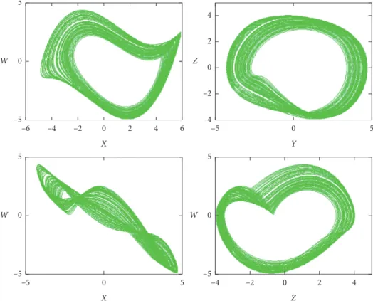
When a � 0.8, b � 0.5, c � 1, d � 0.1,and the initial value is (0.01, 0.01, 0, 0), system (1) produces strange attractors, and the phase trajectory is shown in Figure 2. Using the fourth-order Runge–Kutta integrator, the time step is se-lected to be 0.005, MATLAB is used to solve the equations,

the Lyapunov exponents are L1�0.0357, L2�0, L3�0,

L₄� −0.5357, and Kaplan–Yorke dimension is DKY�3 − ((L₁+ L₂+ L₃)/L4) �3.0666 proving that the system is

chaotic.

2.2. Equlibira Analysis. Solving equation (3), y �0, z �0, w �0, −az − bw − y c −􏼐 dx2􏼑 �0. ⎧ ⎪ ⎪ ⎪ ⎪ ⎪ ⎨ ⎪ ⎪ ⎪ ⎪ ⎪ ⎩ (3)

Therefore, system (1) has a line of equilibria (x, 0, 0, 0). The characteristic equation is

λ λ􏼐 3+ bλ2+ aλ + c − dx2􏼑 �0, (4) where a, b, c, and d are constants and x is an arbitrary variable. When c − dx2� 0, and the equilibrium points are stable, x � ±√��10 when c � 1, d � 0.1. In fact, from the stability criterion of Routh–Hurwitz,

b> 0, a> 0, c − dx2> 0, ab +dx2− c> 0, ⎧ ⎪ ⎪ ⎪ ⎪ ⎪ ⎨ ⎪ ⎪ ⎪ ⎪ ⎪ ⎩ (5)

and when x ∈ (−√��10, −√�6)∪ (√�6,√��10], the nonzero ei-genvalue of the system is either negative or has a negative real part, and therefore the line of equilibria is stable; otherwise, the equilibria are unstable.

Speciﬁcally, there are four types of stability for the line equlibrium points, as shown in Table 1. When x is in the range of (−∞, −√��10)∪ (√��10, +∞) (the green area I in Figure 3), the eigenvalue consists of a zero, a positive real root, and a pair of conjugate complex numbers with a negative real part, correspondingly the equilibrium points

are saddle foci of index-1. When

x∈ [−√��10, −√�6)∪ (√�6,√��10] (the purple area II in Fig-ure 3), the eigenvalue is shown in Table 1, the equilibrium points belong to the stable node foci. When x � ±√�6(the blue area III in Figure 3), the eigenvalue has a pair of virtual roots, and the equilibrium points are stable which turns to be unstable when a Hopf bifurcation occurs. When x changes in the interval (−√�6,√�6) (yellow area IV in Figure 3), the equilibrium points are saddle foci of index-2.

2.3. Bifurcation Analysis. When b � 0.5, c � 1, d � 0.1; the initial value is (0.01, 0.01, 0, 0); and a varies in the range of [0.78, 0.9], system (1) shows a typical inverse period-doubling bifurcation. From the Lyapunov exponent spectrum and bi-furcation diagram in Figure 4, we can see that when the parameter a is in the range of [0.780, 0.788] and [0.791, 0.805], the system returns chaos. When a is in the range of [0.790, 0.791], the cycle-3 attractor is generated in a very short window. When a changes in the region of [0.817, 0.840] and [0.864, 0.900], cycle-2 and cycle-1 are generated, respectively.

(3)

2 1 0 –1 W (x) –2 –5 0 x 5 c = 1, d = 0.1 c = 0.8, d = 0.3 c = 0.6, d = 0.5 (a) 4 2 0 –2 C ur ren t (A) –4 –2 –1 0 1 Voltage (V) 2 f = 0.1hz f = 0.15hz f = 0.3hz (b) Figure 1: The memductance and pinched hysteresis loop.

5 0 W –5 –6 –4 –2 0 X 2 4 6 Y 4 0 2 –2 Z –4 –5 0 5 5 0 W –5 –5 0 X 5 Z 5 0 W –5 –4 –2 0 2 4

Figure 2: Strange attractor projection on various planes of system (1) with (a) � 0.8, (b) � 0.5, c � 1, (d) � 0.1 under the initial condition IC � (0.01, 0.01, 0, 0).

Table 1: The stability of the equilibrium points and corresponding eigenvalues.

x Speciﬁc value Eigenvalue Stability

(−∞, −√��10)∪ (√��10, +∞) x � ± 5 0, 0.8079, −0.6540 ± 1.1954i Region I saddle foci of index-1

±√��10 x � ±√��10 0, 0, −0.25 ± 0.8588i Region II stable node foci

(−√��10, −√�6)∪ (√6�,√��10) x � ± 3 0, −0.1331, −0.1834 ± 0.8471i —

±√�6 x � ±√�6 0, −0.5, ± 0.8944i Region III Hopf bifurcation

(4)

The phase trajectories of system (1) under diﬀerent parameters of a are shown in Figure 5.

When the initial value is (0.01, 0.01, 0, 0), the parameters a, c, and d are set to be 0.8, 1, and 0.1, respectively; while b changes within the range of [0.45, 0.56], system (1) also shows the inverse period-doubling bifurcation. The Lya-punov exponent spectrum and bifurcation diagram of sys-tem (1) are shown in Figure 6. The parameter b in the range of [0.450, 0.492] and [0.495, 0.502] also give the chance for chaos producing. The cycle-2 attractor exists when the pa-rameter b changes in the interval of [0.510, 0.523]. Papa-rameter b generates cycle-1 attractor in the range of [0.532, 0.560]. Corresponding phase trajectories of system (1) are shown in Figure 7.

Under the same initial value, and a � 0.8, b � 0.5, d � 0.1, the Lyapunov exponent spectrum and bifurcation diagram of system (1) are shown in Figure 8. The parameter c in the range of [0.85, 1.1] leads a typical period-doubling bifur-cation, the system gradually changes from periodic state to chaotic state, and the trajectories of system (1) are shown in Figure 9. When the parameter c is in the range of [0.995,

1.011] and [1.016, 1.100], the system is in a chaotic state. When the value of c is changed in the range of [0.947, 0.980] and [0.850, 0.946], cycle-2 attractors and cycle-1 attractors are produced respectively.

2.4. Multistability Observation. The chaotic system is very sensitive to the initial value showing extreme multistability, which can be clearly seen from the Lyapunov exponent spectrum and bifurcation diagram under the control of initial condition x0 or y0 in Figures 10 and 11. When the initial conditions x0 and y0 change within the interval of

[−0.11, 0.11] and [−0.18, 0.15], intermittent chaotic oscil-lations show up. Figures 12 and 13 show the typical phase trajectories under diﬀerent initial values x0 and y0. As

analyzed above, when the parameters are a � 0.8, b � 0.5, c � 1, d � 0.1 and x₀ is in the region of[−√��10, −√�6)∪ (√�6,√��10], the system has inﬁnitely many stable equilibrium points. In this case, we can say inﬁnitely many point attractors coexist with chaotic attractors and periodic attractors.

0 –0.1 –0.2 –0.3 –0.4 LEs –0.5 –0.6 0.8 0.85 a 0.9 6 5.5 5 xmax 0.8 0.85 a 0.9

Figure 4: Lyapunov exponent spectrum and bifurcation diagram of system (1) with (b) � 0.5, (c) � 1, (d) � 0.1 and initial condition IC � (0.01, 0.01, 0, 0), when (a) varies in [0.78, 0.9].

I –5 –1 –0.5 Real ( λi ) 0 0.5 λ2 λ3,4 1 –√10 –√6 0 5 X √6 √10 I II IV II Hopf bifurcation III III

(5)

Furthermore, from the bifurcation diagram of xmaxin Figure 10, system (1) switches its dynamics from period to chaos at the breakpoint of x0�0.02. This discontin-uous bifurcation mode is also proved by Figure 12, where system (1) switches the oscillation from a limit cycle to chaos. Note that all the bifurcation is realized by the initial condition, and therefore the hidden bifurcation occurs in the initial space indicating a new regime of multistability.

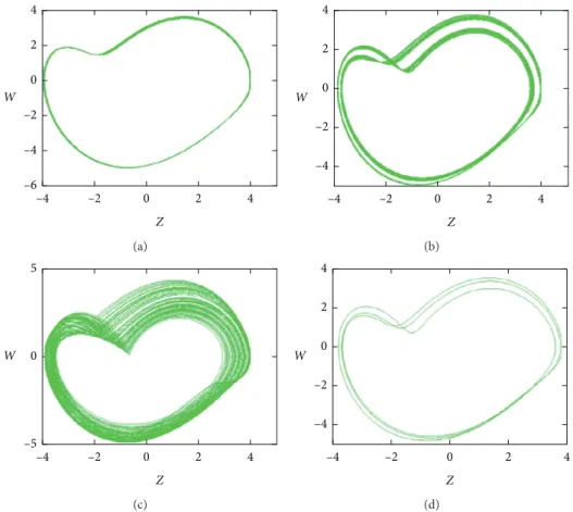
2.5. Amplitude Control. For a dynamical system, there are various parameters influencing the dynamics, some of which are bifurcation ones and some define the geometric prop-erties. In the chaotic system with only one linear or non-linear term, the coefficient of it may play the role of amplitude control. Here, after the tertiary magnetron memristor was introduced into the Jerk system, the new chaotic system introduces only a nonlinear term with a parameter for adjusting the amplitude. When a � 0.8, b � 0.5, 4 2 0 –2 –4 –6 –4 –2 0 2 Z W 4 (a) W –4 –2 0 2 Z 4 4 2 0 –2 –4 (b) 5 0 –5 –4 –2 0 2 Z W 4 (c) W –4 –2 0 2 Z 4 4 2 0 –2 –4 (d)

Figure 5: Typical phase portraits of system (1) with (b) � 0.5, (c) � 1, (d) � 0.1 and IC � (0.01, 0.01, 0, 0) on the (z)-(w) plane: (a) (a) � 0.88, (b) (a) � 0.8306, (c) (a) � 0.8, (d) (a) � 0.7904.

0 –0.1 –0.2 –0.3 –0.4 LEs –0.5 –0.6 6 5 3 2 4 xmax 0.45 0.5 b 0.55 0.45 0.5 b 0.55

Figure 6: Lyapunov exponent spectrum and bifurcation diagram of system (1) with (a) � 0.8, (c) � 1, (d) � 0.1 and initial condition IC � (0.01, 0.01, 0, 0), when (b) varies in [0.45, 0.56].

(6)

c � 1, let x ⟶ (x/√��d), y ⟶ (y/√��d), z ⟶ (z/√��d), w⟶ (w/√��d); the derived equation is the same as system (1) when d � 1, so the coeﬃcient d in system (1) can control the amplitude of the state variables x, y, z, w. The amplitude adjustment of the chaotic attractor is realized by the internal parameter d in the memristor. The parameter d makes the state variables x, y, z, w scaled by the ratio of√��d. As shown in

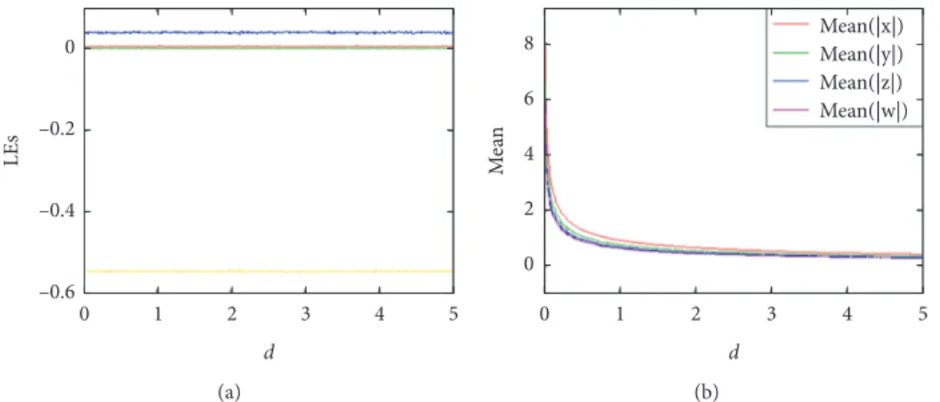
Figure 14, parameter d has basically the same inﬂuence on the amplitude of system state variables x, y, z, and w.

The average value of the absolute value of the state variable decreases with the increase of the parameter d, but when the parameter d changes in the range of [0, 5], the Lyapunov exponent spectrum remains constant. The con-trolled amplitude can be clearly seen from the attractor and 4 2 0 –2 W –4 –4 –2 0 Z 2 4 (a) 4 2 0 –2 W –4 –4 –2 0 Z 2 4 (b) 5 0 W –5 –4 –2 0 Z 2 4 (c) 6 4 2 0 –2 W –4 –6 –5 0 Z 5 (d)

Figure 7: Phase portraits of system (1) with (a) � 0.8, (c) � 1, (d) � 0.1 and initial condition IC � (0.01, 0.01, 0, 0) on the (z)-(w) plane: (a) (b) � 0.55, (b) (b) � 0.52, (c) (b) � 0.5, (d) (b) � 0.4805. 0.2 0 –0.2 –0.4 LEs –0.6 0.9 1 c 1.1 7 6 5 4 xmax 3 0.9 1 c 1.1

Figure 8: Lyapunov exponent spectrum and bifurcation diagram of system (1) with (a) � 0.8, (b) � 0.5, (d) � 0.1 and initial condition IC � (0.01, 0.01, 0, 0), when (c) varies in [0.85, 1.1].

(7)

signal waveforms as shown in Figures 15 and 16. Figures 14–16 show that the size of the attractor has a negative proportion with the parameter d.

3. FPGA-Based Implementation

In this part, digital implementation of the memristive hyperjerk chaotic system is shown. From the variety of digital platform, we choose FPGA technology as this provides a good performance and higher design ﬂexibility. FPGA will also provide a better computing performance with low cost as

when compared to ASIC (Application Specific Integrated Circuits) Technology. FPGA implementation of memristive hyperjerk chaotic system has been implemented and power efficiency analysis is investigated. All four states of a hyperjerk system are discretized using a suitable numerical method (Euler’s method) with 32-bit IEEE-754-1985 floating point format. We have used the hardware-software cosimulation to implement the memristive hyperjerk oscillator in Kintex-7 board and the output is seen using MATLAB.

FPGA-based hyperjerk chaotic system has been obtained using Xilinx (Vivado) system generator [44, 45] which is 2 0 –2 –4 –4 –2 0 Z 2 4 W (a) 4 2 0 –2 W –4 –4 –2 0 Z 2 4 (b) 5 0 W –5 –4 –2 0 Z 2 4 (c) 6 4 2 0 –2 W –4 –6 –5 0 Z 5 (d)

Figure 9: Typical phase portraits of system (1) with (a) � 0.8, (b) � 0.5, (d) � 0.1 and initial condition IC � (0.01, 0.01, 0, 0) on the (z)-(w) plane: (a) (c) � 0.9, (b) (c) � 0.96, (c) (c) � 1, (d) (c) � 1.05. 0 –0.2 –0.4 LEs –0.6 –0.1 –0.05 0 x0 0.05 0.1 6 5 3 4 xmax 2 –0.1 –0.05 0 x0 0.05 0.1

Figure 10: Dynamical evolution of system (1) with (a) � 0.8, (b) � 0.5, (c) � 1, (d) � 0.1 and initial condition IC � (x0, 0, 0.01, 0), and x0varies in [−0.11, 0.11]: (a) Lyapunov exponent spectrum and (b) bifurcation diagram.

(8)

integrated with MATLAB software. Xilinx block sets which are available on the system generator toolbox need to be conﬁgured with zero latency and 32/16-bit ﬁxed point

settings. In order to reduce the bit latency, the output block is conﬁgured to round quantization. By conﬁguring all blocks and setting, the following phase portraits are obtained. 0 –0.2 –0.4 LEs –0.6 –0.1 0 0.1 y0 xmax 6 4 2 –0.1 0 0.1 y0

Figure 11: Dynamical evolution of system (1) with (a) � 0.8, (b) � 0.5, (c) � 1, (d) � 0.1 and initial condition IC � (0.01, y0, 0, 0), and y0varies in [-0.18, 0.15]: (a) Lyapunov exponent spectrum and (b) bifurcation.

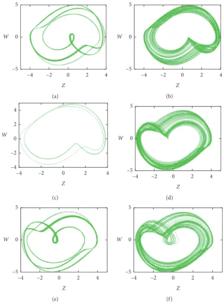
5 W 0 –5 –4 –2 0 Z 2 4 (a) 5 W 0 –5 –4 –2 0 Z 2 4 (b) 2 4 W ₀ –4 –2 –4 –2 0 Z 2 4 (c) 0 5 W –5 –4 –2 0 Z 2 4 (d) 0 5 W –5 –4 –2 0 Z 2 4 (e) 0 5 W –5 –4 –2 0 Z 2 4 (f)

Figure 12: Typical coexisting attractors of system (1) with (a) � 0.8, (b) � 0.5, (c) � 1, (d) � 0.1 and initial condition IC � (x0, 0, 0.01, 0): (a) x0 � −0.0874, (b) x0 � −0.06, (c) x0 �0.002, (d) x0 �0.05, (e) x0 �0.08, (f ) x0 �0.105.

(9)

Figure 17 represents the phase portrait where the hyperjerk chaotic system signals x, y, z, and w are repre-sented with 32 bits using the Forward Euler method by setting h � 0.01 with parameter values a � 0.8, b � 0.5, c � 1, d � 0.1 and the initial condition of (x₀�0.01, y0�0.01, z0�0, w0�0). It can be seen that the

functional hardware results are very similar to MATLAB results. Figure 18 represents the phase portraits of system (1) with a � 0.8, b � 0.5, c � 1, under the initial condition of (0(0.01/􏽰��(0.1/d)), (0.01/􏽰��(0.1/d)),0, 0). D � 0.08 is red while the initial conditions are (0.0089, 0.0089, 0, 0); d �

0.12 is blue while the initial conditions are

(0.0109, 0.0109, 0, 0); and d � 0.25is green while the initial conditions are (0.0158, 0.0158, 0, 0).

Figure 19 and Table 2 show power utilization and re-source utilization of memristive hyperjerk chaotic system

obtained using FPGA with the parameter values,

a �0.08b � 0.5c � 1.05,d � 0.1 under the initial condition (0.01, 0.01, 0, 0).

The power chart of the proposed system gives us in-formation about the diﬀerent resources and their power utilization. From the chart, it is observed that the power consumption is extremely less when compare with realizing the system on other digital software.

0 –0.2 –0.4 LEs –0.6 0 1 2 3 d 4 5 (a) 8 6 4 2 Me an 0 0 1 2 3 d 4 Mean(|x|) Mean(|y|) Mean(|z|) Mean(|w|) 5 (b) Figure 14: Dynamical evolution of system (1) with (a) � 0.8; (b) � 0.5; (c) � 1 and initial condition ((0.01/

�� (0.1/d) 􏽰

), (0.01/􏽰��(0.1/d)), 0, 0), when (d) varies in [0, 5]: (a) Lyapunov exponent spectrum and (b) average values of the absolute value of the chaotic signal.

5 0 W –5 –4 –2 0 2 4 Z (a) 5 0 W –5 –4 –2 0 2 4 Z (b) 5 0 W –5 –4 –2 0 2 4 Z (c) 5 0 W –5 –4 –2 0 2 4 Z (d) –5 5 0 W –4 –2 0 2 4 Z (e) –5 5 0 W –4 –2 0 2 4 Z (f)

Figure 13: Typical coexisting attractors of system (1) with (a) � 0.8, (b) � 0.5, (c) � 1, (d) � 0.1 and initial condition IC � (0.01, y0, 0, 0): (a)y0 �-0.15, (b) y₀ � −0.1185, (c) y₀ � −0.04, (d) y₀ �0.04, (e) y₀ �0.085, and (f ) y₀ �0.13.

(10)

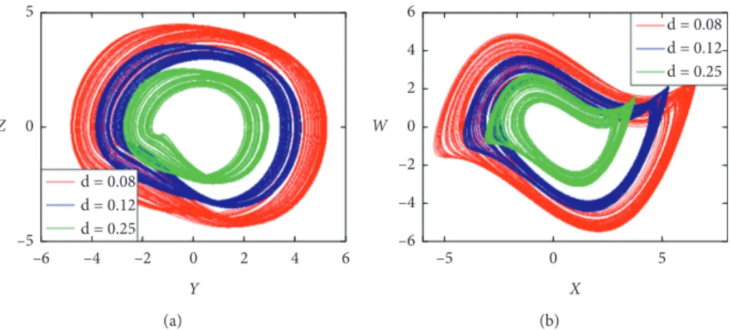
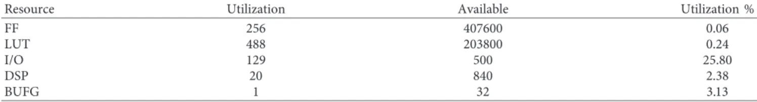
Figure 20 and Table 3 show power utilization and re-source utilization of memristive hyperjerk chaotic system which is obtained using FPGA with the parameter values, a �0.08, b �0.5, c �1.05 under initial condition (0.01/􏽰��(0.1/d)), (0.01/􏽰��(0.1/d)), 0, 0) (a) y-z plane, for d � 0.08 (red), for d � 0.12 (blue), for d � 0.25 (green) (b) x-wplane, for d � 0.08 (red), for d � 0.12 (blue), for d � 0.25 (green).

From Table 3, we can find the different resources such as flip-flops, lookup tables, input-output, digital signal pro-cessing, and the global buffer. The total number of available flip flops in the design is 407600, but here the system had utilized only 0.06% of the available resources, likewise, for other resources too, it had utilized only less numbers; thus, it consumes less power.

The Register-Transfer Level (RTL) schematic of the memristive hyperjerk chaotic system is shown in Figure 21. This RTL design is achieved by interfacing the Xilinx system generator with the Vivado design tool. Each block in the Simulink will get implemented and synthesized using Vivado and generates a schematic diagram. Figure 21 shows the RTL design of the state w of system (1). Kintex 7 is the hardware chosen to implement the system.

4. System Prediction with Artificial

Neural Network

ANN is a mathematical model representing neurons in the brain and their network relationships [35]. In ANN archi-tecture design, the number of layers, the number of neurons in the layers, the learning algorithm, and activation func-tions are parameters that can be changed to achieve the desired result. A basic neuron model is given in Figure 22. Inputs are denoted by x, outputs are denoted by y, weights are denoted by w, bias is denoted by b, and f denotes ac-tivation function. The neuron output is given in Table 4 [42]. Each input information is multiplied by weight and added by bias. The output (y) is obtained by processing the total value on the activation function.

yj � f 􏽘

n

xnwn+ b ⎛

⎝ ⎞_⎠. ₍₆₎

Chaotic data can be predicted with artiﬁcial neural networks. Compared with the fuzzy logic method [38] or the fuzzy neural network [39], NARX network model can give d = 0.08 d = 0.12 d = 0.25 5 0 –5 Z –6 –4 –2 0 2 Y 4 6 (a) d = 0.08 d = 0.12 d = 0.25 6 4 2 W 0 –2 –4 –6 –5 0 X 5 (b)

Figure 15: Phase trajectories of system (1) with (a) � 0.8; (b) � 0.5; (c) � 1 under the initial condition ((0.01/ �� (0.1/d) 􏽰

), (0.01/􏽰��(0.1/d)), 0, 0): (a) (y)-(z) plane and (b) (x)-(w) plane.

d = 0.08 d = 0.12 d = 0.25 5 0 –5 x ( t) 500 1000 Time (Sec) 1500 2000 (a) d = 0.08 d = 0.12 d = 0.25 500 1000 Time (Sec) 1500 2000 6 4 2 z ( t) ₀ –2 –4 –6 (b)

(11)

the prediction in a relatively simple way [46]. NARX is a feedforward network model with two layers. A general di-agram of the NARX model is given in Figure 23 [46]. In the ﬁrst layer (Layer 1), data from inputs and outputs enter the network by passing through the delay line (TDL-Tapped Delay Time). Thus, the past values of the time series are also applied to the input. In the NARX model, the network architecture relates both the present value of the time series and the current and past values of the exogenous input [46].

The mathematical expression of the input and output re-lationship of the NARX model is given in equation (7) [46, 47].where u is the input, y is the output, m and n are the number of input and output variables, f1 _{and f}2 _{are the}

activation functions, IW is the input weight, LW is the output weight, b1is the Layer-1 bias (input bias), b2is the Layer-2 bias (output bias), and t is the time step. In Fig-ure 23, Layer-1 refers to the hidden layer, and Layer-2 refers to the output layer. Equation (8) gives the dynamics of the 5 0 –5 –4 –2 0 2 X 4 6 W (a) –5 0 5 Y 4 2 0 –4 –2 Z (b) –5 0 Y 5 5 0 –5 W (c) Z –4 –2 0 2 4 5 0 –5 W (d)

Figure 17: Strange attractor projections on various planes of system (1) with (a) � 0.8, (b) � 0.5, (c) � 1, (d) � 0.1under the initial condition (0.01, 0.01, 0, 0). 5 0 –5 –6 –4 –2 Y Z 0 2 4 (a) X W 6 4 2 0 –4 –2 –5 0 5 (b)

Figure 18: Phase portraits of system (1) with (a) � 0.08, (b) � 0.5, (c) � 1.05, under the initial condition ((0.01/ �� (0.1/d) 􏽰

), (0.01/􏽰��(0.1/d)), 0, 0), (d) � 0.08 is red, (d) � 0.12 is blue, (d) � 0.25 is green (a) (y)-(z) plane, (b) (x)-(w) plane.

(12)

NARX network for the number of q neurons. In equation (8), i indicates the index of neurons and j indicates the index of n inputs [46]:

y(t) � f[[u(t), u(t −Δt), . . . , u(t − mΔt),

y(t −Δt), . . . , y(t − nΔt)], (7) Clocks: 0.163 W (51%) (2%) 9% 10% 75% 100% 49% 51% (9%) (4%) (10%) (75%) (49%) (100%) 0.003 W 0.015 W 0.007 W 0.017 W 0.122 W 0.159 W 0.159 W Signals: Logic: DSP: I/O: PL static: Static: Dynamic:

Figure 19: Power consumed for the FPGA implementation of memristive hyperjerk chaotic system (1).

Table 2: Resource utilization for the FPGA implementation of memristive hyperjerk chaotic system.

Resource Utilization Available Utilization %

FF 256 407600 0.06 LUT 488 203800 0.24 I/O 129 500 25.80 DSP 20 840 2.38 BUFG 1 32 3.13 Clocks: 0.163 W (51%) (2%) 9% 10% 75% 100% 49% 51% (9%) (4%) (10%) (75%) (49%) (100%) 0.003 W 0.015 W 0.007 W 0.017 W 0.122 W 0.159 W 0.159 W Signals: Logic: DSP: I/O: PL static: Static: Dynamic:

Figure 20: Power consumed for the FPGA implementation of memristive hyperjerk chaotic system (1).

Table 3: Resource utilization for the FPGA implementation of memristive hyperjerk chaotic system.

Resource Utilization Available Utilization %

FF 256 407600 0.06

LUT 495 203800 0.24

I/O 129 500 25.80

DSP 20 840 2.38

(13)

Figure 21: The RTL schematic of memristive hyperjerk chaotic system implemented in Kintex-7 using hardware-software cosimulation. w1 w2 x1 x2 w3 wn _b ∑ f y x3 xn

Figure 22: A basic neuron model [37].

Table 4: The performance of the network in diﬀerent learning algorithms and diﬀerent hidden layer neuron numbers.

Learning algorithm Number of hidden layer neurons Test performance value (mse)

Levenberg–Marquardt 5 4.7493e-08

Bayesian regularization 5 5.3542e-09

Scaled conjugate gradient 5 4.1850e-04

(14)

x (t) y (t) W W W b 4 y (t) 4 20 Output Hidden + + b 1:2 1:2 4 4

Figure 24: The designed NARX model.

1000 epochs 0 200 10–10 10–5 M ea n s qua re d er ro r (m se ) 100 400 600 800 1000 (a) 14000 12000 10000 In st an ces ₈₀₀₀ 6000 4000 2000 Errors

Error histogram with 20 bins

0

–0.00016 –0.00015 –0.00013 –0.00012 –0.0001 –8.7e–05 –7.1e–05 –5.6e–05 –4e–05 –2.5e–05 –9.6e–06 5.8e–06 2.12e–05 3.66e–05 5.2e–05 6.73e–05 8.27e–05 9.81e–05 0.000114 0.000129

Zero error (b)

Figure 25: For tested network: (a) performance (mse values), (b) error histogram.

T D L IW1,1 _LW2,1 LW1,3 S1_{× R} R1_{× 1} p1_{(t) = u(t)} a2_{(t) = y}^_(t) a1_(t) n1_(t) n2_(t) 1 + +

Inputs Layer-1 Layer-2

R1 _S1_{× 1} b1 _b2 f1 _f2 1 _S1_{× 1} S2_{× 1} S2_{× 1} S2_{× 1} S2_{× S}1 S1 _S2 S1_{× 1} T D L

(15)

y(t) � f2 b2+ 􏽘 q i�1 LW_if1 b1+ 􏽘 n j�1 IW_iju_jt ⎡ ⎢ ⎢ ⎣ ⎤⎥⎥⎦ ⎧ ⎪ ⎨ ⎪ ⎩ ⎫ ⎪ ⎬ ⎪ ⎭. (8)

The designed NARX model given in Figure 24 is used to estimate the system (1) with ANN. The network model has 4 inputs (x, y, z, w) and 4 outputs (x∧, y∧, z∧, w∧_{). The data}

obtained from the simulation result under the initial conditions (0.01, 0.01, 0, 0) of system (1) are used as the data set. 24500 of the data set are used for training (70% of the data set), 5250 of the

data set used for validation (15% of the data set), and 5250 of the data set used for testing (15% of the data set). Training, testing, and verification data are taken at random. 15000 pieces of data that were not given to the network before were used for testing. Hyperbolic tangent is used as the activation function in the hidden layer, and a pureline function is used as the activation function in the output layer. Three different learning algorithms, Levenberg-Marquardt, Bayesian Regularization, and Scaled Conjugate Gradient are used for network training. The per-formance of the network is compared using three different training algorithms by taking the number of hidden layer 5 0 –5 –5 0 X W 5 (a) 5 0 –5 –5 0 ~X ~W 5 (b) 5 0 –5 –5 0 Y Z 5 (c) 5 0 –5 –5 0 ~Y ~Z 5 (d) 5 0 –5 –5 0 Y W 5 (e) 5 0 –5 –5 0 ~Y ~W 5 (f ) 5 0 –5 –5 0 Z W 5 (g) 5 0 –5 –5 0 ~Z ~W 5 (h)

(16)

neurons at different values. The performance (mse-mean squared error) of the network in different learning algorithms and different numbers of hidden layer neuron is given in Table 4. As can be seen from Table 4, the best result was achieved with the Levenberg–Marquardt learning algorithm and 20 neurons in the hidden layer. Performance (mse values) and error histogram graphs of the tested network are given in Figure 24. In the test simulation process, the mse value was obtained as 9.1743e-10, Figure 25(a). As a result, according to this mse value, the trained network can predict the chaotic system (1) very well.

As can be seen from the phase portraits in Figure 26, designed ANN has predicted system (1) very successfully. The green attractors and blue attractors represent the target data and the predicted data from the artiﬁcial neural net-work, respectively.

5. Conclusion

When a memristor is introduced into a jerk structure, a new memristive hyperjerk chaotic system with amplitude control is designed. The coeﬃcient of the internal variable shows its function for amplitude control. In this work, it is proven that the jerk structure can host a nonlinear memristor for chaos rescaling. By revising, a resistor in the physical circuit can realize the total amplitude control leaving much margin for chaos application. Like some of the other memristive chaotic systems [48–50], the newly proposed chaotic system shows extreme multistability. The implementation of FPGA proves the consistence of theoretical analysis and numerical sim-ulation. Also, the proposed memristive hyperjerk chaotic system is predicted with ANN for AI based engineering applications. Further work associated with this system like chaos-based communication or image encryption is ex-pected in the near future.

Data Availability

The data used to support the ﬁndings of this study are available from the corresponding author upon reasonable request.

Conflicts of Interest

The authors declare that there are no conﬂicts of interest regarding the publication of this paper.

Acknowledgments

This work was supported ﬁnancially by the National Natural Science Foundation of China (Grant no. 61871230), the Natural Science Foundation of Jiangsu Province (Grant no. BK20181410), and a Project Funded by the Priority Aca-demic Program Development of Jiangsu Higher Education Institutions.

References

[1] S. He, K. Sun, Y. Peng, and L. Wang, “Modeling of discrete fracmemristor and its application,” AIP Advances, vol. 10, no. 1, 2020.

[2] S. Wen, R. Hu, Y. Yang et al., “Memristor based echo state network with online least mean square,” IEEE Transactions on

Systems, Man and Cybernetics, vol. 49, no. 9, pp. 1787–1796, 2019.

[3] C. Li, J. C. Thio, H. H. C. Iu et al., “A memristive chaotic oscillator with increasing amplitude and frequency,” IEEE

Access, vol. 6, pp. 12945–12950, 2018.

[4] Q. Lai, Z. Wan, L. K. Kengne, P. D. K. Kuate, and C. Chen, “Two-memristor-based chaotic system with inﬁnite coexist-ing attractors,” IEEE Transactions on Circuits and Systems II:

Express Briefs, 2020.

[5] S. T. Kingni, C. Ainamon, V. V. Tamba, and B. C. Orou, “Directly modulated semiconductor ring lasers: chaos synchronization and applications to cryptography communications,” Chaos Theory

and Applications, vol. 2, no. 1, pp. 31–39, 2020.

[6] A. S. K. Tsafack, R. Kengne, A. Cheukem, J. R. M. Pone, and G. Kenne, “Chaos control using self-feedback delay controller and electronic implementation in IFOC of 3-phase induction motor,” Chaos Theory and Applications, vol. 2, no. 1, pp. 40–48, 2020.

[7] J. C. Sprott, “Do we need more chaos examples?” Chaos

Theory and Applications, vol. 2, no. 2, pp. 49–51, 2020.

[8] Q. Lai, N. Benyamin, and L. Feng, “Dynamic analysis, circuit realization, control design and image encryption application of an extended l¨u system with coexisting attractors,” Chaos

Solitons & Fractals, vol. 114, pp. 230–245, 2018.

[9] Q. Lai, P. D. K. Kuate, F. Liu, and H. C. Lu, “An extremely simple chaotic system with inﬁnitely many coexisting attractors,” IEEE Transactions on Circuits and Systems II:

Express Briefs, vol. 67, 2019.

[10] C. Li and J. C. Sprott, “Multistablility in a butterﬂy ﬂow,”

International Journal of Bifurcation and Chaos, vol. 23, no. 12,

2013.

[11] S. He, B. Yan, and S. Wang, “Multistability and formation of spiral waves in a fractional-order memristor-based hyper-chaotic l¨u system with No equilibrium points,” Mathematical

Problems in Engineering, vol. 2020, Article ID 2468134,

12 pages, 2020.

[12] X. Zhang and C. Wang, “A novel attractor period multi-scroll chaotic integrated circuit based on CMOS wide ad-justable CCCII,” IEEE Access, vol. 7, no. 1, pp. 16336–16350, 2019.

[13] C. Li and J. C. Sprott, “Amplitude control approach for chaotic signals,” Nonlinear Dynamics, vol. 73, no. 3, pp. 1335–1341, 2013.

[14] C. Li, J. C. Sprott, and H. Xing, “Crisis in amplitude control hides in multistability,” International Journal of Bifurcation

and Chaos, vol. 26, no. 14, Article ID 1650233, 2016.

[15] Z. Gu, C. Li, X. Pei et al., “A conditional symmetric mem-ristive system with amplitude and frequency control,” The

European Physical Journal Special Topics, vol. 229, pp. 1007–

1019, 2015.

[16] E. Dong, Z. Liang, S. Du et al., “Topological horseshoe analysis on a four-wing chaotic attractor and its FPGA implement,”

Nonlinear Dynamics, vol. 83, pp. 623–630, 2016.

[17] E. Tlelo-Cuautle, J. Rangel-Magdaleno, A. Pano-Azucena et al., “FPGA realization of multi-scroll chaotic oscillators,”

Communications in Nonlinear Science and Numerical Simu-lation, vol. 27, pp. 66–80, 2015.

[18] K. Rajagopal, A. Karthikeyan, and A. K. Srinivasan, “FPGA implementation of novel fractional-order chaotic systems with two equilibriums and no equilibrium and its adaptive sliding mode synchronization,” Nonlinear Dynamics, vol. 87, pp. 1–24, 2016.

(17)

[19] E. Tlelo-Cuautle, A. D. Pano-Azucena, and J. J. Rangel-Magdaleno, “Generating a 50-scroll chaotic attractor at 66MHzby using FPGAs,” Nonlinear Dyn, vol. 85, no. 4, pp. 2143–2157, 2016.

[20] Q. Wang, S. Yu, C. Li et al., “Theoretical design and FPGA-based implementation of higher-dimensional digital chaotic systems,” IEEE Transactions on Circuits and Systems I: Regular

Papers, vol. 63, no. 3, pp. 401–412, 2016.

[21] A. Karthikeyan, K. Rajagopal, V. Sundarapandian et al., “Chaos control in fractional order smart grid with adaptive sliding mode control and genetically optimized PID control and its FPGA implementation,” Complexity, vol. 2017, Article ID 3815146, 18 pages, 2017.

[22] ˙I. Koyuncu, ˙I. S¸ahin, C. Gloster et al., “A neuron library for rapid realization of artiﬁcial neural networks on FPGA: a case study of r¨ossler chaotic system,” Journal of Circuits, Systems

and Computers, vol. 26, Article ID 1750015, 2017.

[23] M. Alçın, ˙I. Pehlivan, and ˙I. Koyuncu, “Hardware design and implementation of a novel ANN-based chaotic generator in FPGA,” International Journal for Light and Electron Optics, vol. 127, pp. 5500–5505, 2016.

[24] S. Mobayen and J. Ma, “Robust ﬁnite-time composite non-linear feedback control for synchronization of uncertain chaotic systems with nonlinearity and time-delay,” Chaos,

Solitons & Fractals, vol. 114, pp. 46–54, 2018.

[25] G. Cheng, C. Wang, and H. Chen, “A novel color image en-cryption algorithm based on hyperchaotic system and permu-tation-diﬀusion architecture,” International Journal of Bifurcation and Chaos, vol. 29, no. 09, Article ID 1950115, 2019.

[26] B. Alatas, E. Akin, and A. B. Ozer, “Chaos embedded particle swarm optimization algorithms,” Chaos, Solitons & Fractals, vol. 40, no. 4, pp. 1715–1734, 2009.

[27] G. I. Sayed, A. Darwish, and A. E. Hassanien, “A new chaotic multi-verse optimization algorithm for solving engineering optimization problems,” Journal of Experimental &

Theo-retical Artiﬁcial Intelligence, vol. 30, no. 2, pp. 293–317, 2018.

[28] G. Kaur and S. Arora, “Chaotic whale optimization algo-rithm,” Journal of Computational Design and Engineering, vol. 5, no. 3, pp. 275–284, 2018.

[29] Z. B. Garip, M. E. Cimen, D. Karayel et al., “The Chaos-based whale optimization algorithms global optimization,” Chaos

Teory and Application, vol. 1, no. 1, pp. 51–63, 2019.

[30] L. J. Yang and T. L. Chen, “Application of chaos in genetic algorithms,” Communications in Theoretical Physics, vol. 38, no. 2, pp. 168–172, 2002.

[31] P. Snaselova and F. Zboril, “Genetic algorithm using theory of chaos,” Procedia Computer Science, vol. 51, pp. 316–325, 2015. [32] X. Yuan, Y. Yuan, and Y. Zhang, “A hybrid chaotic genetic algorithm for short-term hydro system scheduling,”

Mathe-matics and Computers in Simulation, vol. 59, no. 4, pp. 319–

327, 2002.

[33] R. Ebrahimzadeh and M. Jampour, “Chaotic genetic algo-rithm based on Lorenz chaotic system for optimization problems,” International Journal of Intelligent Systems and

Applications, vol. 5, no. 5, pp. 19–24, 2013.

[34] D. S. K. Karunasinghe and S.-Y. Liong, “Chaotic time series prediction with a global model: artiﬁcial neural network,”

Journal of Hydrology, vol. 323, no. 1–4, pp. 92–105, 2006.

[35] ˙I. Dalkıran, F. Y. Dalkıran, and R. Kılıç, “Prediction of dy-namics of chaotic Chua’s circuit with artiﬁcial neural net-work,” in Proceedings of the IEEE 15th Signal Processing and

Communications Applications, pp. 1–4, Eskisehir, Turkey, July

2007.

[36] J. W. Woolley, P. K. Agarwal, and J. Baker, “Modeling and prediction of chaotic systems with artiﬁcial neural networks,”

International Journal for Numerical Methods in Fluids, vol. 63,

pp. 989–1004, 2010.

[37] M. K. Rafsanjani and M. Samareh, “Chaotic time series prediction by artiﬁcial neural networks,” Journal of

Compu-tational Methods in Sciences and Engineering, vol. 16, no. 3,

pp. 599–615, 2016.

[38] M. N. Alemu, “A fuzzy model for chaotic time series pre-diction,” International Journal of Innovative Computing,

In-formation and Control, vol. 14, no. 5, pp. 1767–1786, 2018.

[39] M. Han, K. Zhong, T. Qiu, and B. Han, “Interval type-2 fuzzy neural networks for chaotic time series prediction: a concise overview,” IEEE Transactions on Cybernetics, vol. 49, no. 7, pp. 2720–2731, 2019.

[40] M. Alcin, I. Koyuncu, M. Tuna et al., “A novel high speed artiﬁcial neural network-based chaotic true random number generator on ﬁeld programmable gate array,” International

Journal of Circuit Theory and Applications, vol. 47, no. 3,

pp. 365–378, 2019.

[41] S. Vaidyanathan, I. Pehlivan, L. G. Dolvis et al., “A novel ANN-based four-dimensional two-disk hyperchaotic dy-namical system, bifurcation analysis, circuit realisation and FPGA-based TRNG implementation,” International Journal

of Computer Applications in Technology, vol. 62, no. 1,

pp. 20–35, 2020.

[42] ˙I. Dalkiran and K. Danıs¸man, “Artiﬁcial neural network based chaotic generator for cryptology,” Turkish Journal of Electrical

Engineering & Computer Sciences, vol. 18, no. 2, pp. 225–240,

2010.

[43] A. R. Bevi, S. Tumu, and N. V. Prasad, “Design and inves-tigation of a chaotic neural network architecture for cryp-tographic applications,” Computers & Electrical Engineering, vol. 72, pp. 179–190, 2018.

[44] K. Rajagopal, L. Guessas, A. Karthikeyan et al., “Fractional-order memristor no equilibrium chaotic system with its adaptive sliding mode synchronization and genetically opti-mized fractional-order pid synchronization,” Complexity, vol. 2017, Article ID 1892618, 19 pages, 2017.

[45] E. Tlelo-Cuautle, V. H. Carbajal-Gomez, P. J. Obeso-Rodelo, J. J. Rangel-Magdaleno, and J. C. N´uñez-P´erez, “FPGA re-alization of a chaotic communication system applied to image processing,” Nonlinear Dynamics, vol. 82, no. 4, pp. 1879–1892, 2015.

[46] S. A. Taqvi, L. D. Tufa, H. Zabiri, A. S. Maulud, and F. Uddin, “Fault detection in distillation column using NARX neural network,” Neural Computing and Applications, vol. 32, no. 8, pp. 3503–3519, 2020.

[47] J. Buitrago and S. Asfour, “Short-term forecasting of electric loads using nonlinear autoregressive artiﬁcial neural networks with exogenous vector inputs,” Energies, vol. 10, no. 1, 2017. [48] B. Bao, Q. Yang, D. Zhu, Y. Zhang, and M. Chen, “Initial-induced coexisting and synchronous ﬁring activities in memristor synapse-coupled morris–lecar bi-neuron net-work,” Nonlinear Dynamics, vol. 99, no. 3, pp. 1–16, 2020. [49] B. Bao, X. Tan, M. Chen, Y. Zhang, Q. Xu, and H. Bao, “Riddled

attraction basin and multistability in three-element-based memristive circuit,” Complexity, vol. 2020, Article ID 4624792, 13 pages, 2020.

[50] H. Bao, D. Zhu, W. Liu, Q. Xu, and B. Bao, “Memristor synapse-based morris–lecar model: bifurcation analyses and FPGa-based validations for periodic and chaotic bursting/ spiking ﬁrings,” International Journal of Bifurcation and