Copula-based multivariate input modeling

Contents lists available atSciVerse ScienceDirect

Surveys in Operations Research and Management Science

journal homepage:www.elsevier.com/locate/sorms

Review

Copula-based multivariate input modeling

Bahar Biller

a,∗

, Canan Gunes Corlu

b a_{Tepper School of Business, Carnegie Mellon University, United States} b_{Department of Industrial Engineering, Bilkent University, Turkey}

a r t i c l e i n f o

Article history:

Received 7 April 2010 Received in revised form 13 February 2012 Accepted 3 April 2012

a b s t r a c t

In this survey, we review the copula-based input models that are well suited to provide multivariate input-modeling support for stochastic simulations with dependent inputs. Specifically, we consider the situation in which the dependence between pairs of simulation input random variables is measured by tail dependence (i.e., the amount of dependence in the tails of a bivariate distribution) and review the techniques to construct copula-based input models representing positive tail dependencies. We complement the review with the parameter estimation from multivariate input data and the random-vector generation from the estimated input model with the purpose of driving the simulation.

© 2012 Elsevier Ltd. All rights reserved.

Contents

1. Introduction... 69

2. Two measures of dependence: correlation and tail dependence... 70

2.1. Correlation... 70

2.2. Tail dependence... 71

3. Copula-based input modeling... 72

3.1. Fundamentals of copula theory... 73

3.2. Bivariate copula models... 74

3.2.1. Elliptically symmetric copulas... 74

3.2.2. Archimedean copulas... 75

3.2.3. Max-infinitely divisible copulas... 75

3.3. Multivariate copula models... 75

3.3.1. Multivariate elliptical copulas... 75

3.3.2. Exchangeable multivariate Archimedean copulas... 76

3.3.3. Mixtures of max-infinitely divisible copulas... 76

3.3.4. Vines... 77 4. Fitting methods... 78 4.1. Frequentist method... 78 4.2. Bayesian method... 79 5. Goodness-of-fit tests... 80 6. Sampling... 81

6.1. Sampling from the normal copula and the t copula... 81

6.2. Sampling from the Archimedean copulas... 81

6.3. Sampling from theC-vine andD-vine specifications... 81

7. Conclusion... 82

References... 82

1. Introduction

An important step in the design of a stochastic simulation is input modeling; i.e., choosing a probability distribution to

∗_{Corresponding author.}

E-mail address:billerb@andrew.cmu.edu(B. Biller).

represent the inputs of the system being studied. Input modeling is easily performed when the system inputs can be represented as a sequence of independent and identically distributed random variables. Reviews of such input models are available in [1–3].

The focus of this survey is on stochastic simulations with dependent inputs that require the use of flexible multivariate input models to capture their joint distributional properties. Examples

1876-7354/$ – see front matter©2012 Elsevier Ltd. All rights reserved. doi:10.1016/j.sorms.2012.04.001

of dependent inputs in need of multivariate input-modeling support include the processing times of workpieces across work centers [4], the inter-arrival times of file accesses in computer systems [5–7], the medical characteristics of organ-transplant donors and recipients [8], arrival and service processes of Web servers [9], the inter-arrival times of customers in call centers [10], and the product demands and exchange rates of global supply chains [11]. Choosing correlation as the dependence measure, Ghosh and Squillante [9] show that ignoring the correlation between the inter-arrival and service times of Web server queues leads to a 25% overestimation of the waiting times, while assuming independent and identically distributed inter-arrival times leads to the underestimation of the expected waiting times by a factor of four. Clearly, the independence assumption can lead to very poor estimates of the performance measures when there is actually correlation present, and the consequences of ignoring correlation can be severe. A comprehensive review of the multivariate input models measuring dependence by correlation is available in [12]. Patton [13], on the other hand, demonstrates the need for an input model that captures not only the correlation but also the dependence in the tails of the exchange rate processes. What distinguishes our survey from others is its focus on this measure of dependence, which is known as the tail dependence and defined as the amount of dependence in the tails of a joint distribution. Other applications with focus on tail dependence include Corbett and Rajaram [14], Wagner et al. [15], and Tehrani et al. [16], and they demonstrate that it is imperative to develop multivariate input models that can capture stochastic tail dependencies among the input random variables of stochastic systems.

A close look at the existing literature reveals that multivariate input models can be classified into two types: random vectors and multivariate time series. Specifically, a random vector X

=

(

X1

,

X2

, . . . ,

Xk

)

′denotes a collection of k random components, each of which is a real-valued random variable, and it is described by its joint distribution function. A k-dimensional time series Xt

=

{

(

X1,t

,

X2,t

, . . . ,

Xk,t

)

′

;

t

=

1

,

2

, . . .}

, on the other hand, denotes a sequence of random vectors observed at times t

=

1

,

2

, . . .

. In this survey, we focus on random vectors and refer the reader to Biller and Ghosh [12] for a comprehensive review of the time-series pro-cesses for stochastic simulations. More specifically, we consider multi-dimensional copula-based input models that have the ability to capture a wide variety of dependence structures by describing dependence in a more general manner than correlation. The use of correlation as the measure of dependence in the simulation input-modeling research has been justified by the fact that making it possible for simulation users to incorporate dependence via corre-lation, while limited, is substantially better than the practice of ig-noring dependence. However, when the simulation inputs are not jointly elliptically distributed and require the use of a joint prob-ability distribution with positive dependence in the tails, correla-tion is no longer sufficient to describe the dependence structure of these simulation inputs. Therefore, in this survey we go beyond the use of correlation as a dependence measure and present the application of copula theory to multivariate input modeling with the purpose of constructing flexible density models that represent a wide variety of dependence structures. Additionally, we consider the problems of estimating the parameters of the copula-based in-put models from multivariate data and generating random vec-tors with the pre-specified marginal distributions and dependence structures to drive stochastic simulations. We refer the reader to Craney and White [17] for input modeling techniques when no data are available.

We organize the remainder of the paper as follows. In Section2, we introduce correlation and tail dependence as the two measures of dependence that are used for multivariate input modeling with focus on the limitations of correlation as the dependence measure.

In Section 3, we present copula-based input models with the

ability to measure tail dependence; Section 3.1 reviews copula theory, Section3.2focuses on two-dimensional input models, and Section3.3 extends the discussion to multivariate input models

with three or more component random variables. In Section4,

we describe how to estimate the parameters of the copula-based input models from multivariate data via automated algorithms. We present the goodness-of-fit tests specifically designed for copula-based input models in Section5. In Section6, we provide the sampling algorithms that generate random vectors from the copula-based input models quickly and accurately to drive stochastic simulations. We conclude our review with a discussion of promising research areas in Section7.

2. Two measures of dependence: correlation and tail depen-dence

Dependent random vectors are often specified partially in terms of the marginal distributions of their component random variables and pair-wise measures of dependence summarizing how these components interact with each other. Although this may not uniquely or even correctly specify the joint distribution of the random vector, the hope is to find a useful specification for the dependence structure among the components, while sparing the simulation practitioner the task of trying to estimate the full joint distribution. In Section 2.1, we review product-moment correlation and rank correlation as the dependence measures that are often used for this purpose in simulation input modeling. In Section2.2, we introduce tail dependence and motivate its consideration in this survey as a measure of the dependence captured by neither product-moment correlation nor rank correlation. The dependence measures we consider in each of these sections are pair-wise measures, in that they are used to quantify the dependence between the pairs of random variables. It is important to note that, despite the focus of this survey, correlation and tail dependence are not the only means to measure dependence; we refer the reader to Nelsen [18] for a discussion of alternative measures.

2.1. Correlation

The product-moment correlation and the rank correlation are the two widely used measures of dependence in applications of stochastic simulations. Specifically, the rank correlation r

(

i

,

j

)

between random variables Xiand Xjis defined by

r

(

i

,

j

) =

E



Fi

(

Xi

)

Fj

(

Xj

) −

E

(

Fi

(

Xi

))

E



Fj

(

Xj

)



Var

(

Fi

(

Xi

))

Var



Fj

(

Xj

)

,

where Fiis the cumulative distribution function (cdf) of Xi[19]. The product-moment correlation

ρ

X

(

i

,

j

)

between Xiand Xjwith finite variances Var

(

Xi

)

and Var

(

Xj

)

is, on the other hand, given by

ρ

X

(

i

,

j

) =

Cov



Xi

,

Xj





Var

(

Xi

)

Var



Xj



=

E



XiXj

 −

E

(

Xi

)

E



Xj





Var

(

Xi

)

Var



Xj



,

where Cov

(

Xi

,

Xj

)

is the product-moment covariance between Xi and Xj [20]. Thus, a correlation of 1 is the maximum possi-ble for bivariate normal random variapossi-blesΦ−1

(

Fi

(

Xi

)) (≡

Zi

)

and

Φ−1

₍

_F

j

(

Xj

)) (≡

Zj

)

, whereΦis the cdf of a standard normal ran-dom variable. Therefore, taking Cov

(

Zi

,

Zj

) =

1 is equivalent (in distribution) to setting Zi

←

Φ−1

(

U

)

and Zj

←

Φ−1

(

U

)

, where U is a uniform random variable in the interval

(

0

,

1

)

[21]. This def-inition of Ziand Zjimplies that Xi

←

Fi−1

(

U

)

and Xj

←

Fj−1

(

U

)

,

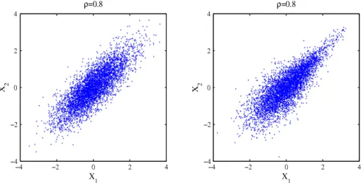
Fig. 1. Input models with standard normal marginals, but with different dependence structures.

from which it follows that

ρ

X

(

i

,

j

)

takes on its maximum

magni-tude. Similarly, taking Cov

(

Zi

,

Zj

) = −

1 is equivalent (in distribu-tion) to setting Xi

←

Fi−1

(

U

)

and Xj

←

Fj−1

(

1

−

U

)

, in which case the correlation

ρ

X

(

i

,

j

)

assumes the minimum possible value for

the random variables Xiand Xj. Furthermore, in the special case of jointly normal input random variables, the product-moment cor-relation

ρ

X

(

i

,

j

)

relates to the rank correlation r

(

i

,

j

)

by

ρ

X

(

i

,

j

) =

2 sin

(π

r

(

i

,

j

)/

6

)

[22].

Despite its wide use, the product-moment correlation suf-fers from several limitations that have motivated simulation practitioners to look for alternative measures of dependence (e.g., [23,12]):

(1) The product-moment correlation cannot capture the nonlinear dependence between random variables. Consequently, it fails to model the non-zero dependence in the tails of a bivariate distribution. As an example, Fig. 1 shows 10 000 bivariate realizations sampled from two different input models constructed for the random vector X

=

(

Xi

,

Xj

)

′. In both of

these models, X_i and X_j have standard normal marginal

distributions and the product-moment correlation

ρ

X

(

i

,

j

)

is

0.8, but with different dependence structures: The first model has the bivariate normal distribution, while the second model has the Gumbel distribution with parameter

θ

that takes the value of 3.8 (Section3.2). More specifically, the dependence in the tails of the joint distribution is zero in the first model, while extreme positive realizations have a tendency to occur together in the second model. Thus, the structure of dependence in the two models cannot be distinguished on the grounds of product-moment correlation alone.

(2) A product-moment correlation of zero between two random variables does not guarantee their independence. For example, the correlation

ρ

X

(

i

,

j

)

is zero between Xi and Xj that are uniformly distributed on the unit circle, but Xi and Xj are dependent as X2

i

+

Xj2

=

1.

(3) A weak product-moment correlation does not imply low dependence. For example, the minimum product-moment correlation between two lognormal random variables with

zero means and standard deviations of 1 and

σ

2 is the

correlation between eZ _{and e}−σZ_{, while the maximum}

product-moment correlation between these two random variables is the correlation between eZ _{and e}σZ_{, where Z is a} standard normal random variable [23]. Although both of these correlations tend to zero with increasing values of

σ

, they are highly dependent.

(4) It follows from the definition of the product-moment correla-tion that

ρ

X

(

i

,

j

)

takes values between

−

1 and 1, but the actual

values

ρ

X

(

i

,

j

)

can assume depends on the marginal

distribu-tions of the input random variables Xiand Xj[24]. For example, the attainable interval for the product-moment correlation of two lognormal random variables with zero means and stan-dard deviations of 1 and 2 is

[−

0

.

090

,

0

.

666

]

; i.e., it is not pos-sible to find a bivariate distribution with these marginals and a product-moment correlation of 0.7.

(5) Product-moment correlation is not invariant under transfor-mations of the input random variables. For example, the product-moment correlation between log

(

Xi

)

and log

(

Xj

)

is not the same as the product-moment correlation between Xiand Xj unless they are independent.

(6) Product-moment correlation is only defined when the vari-ances of the random variables are finite. Therefore, it is not an appropriate dependence measure for heavy-tailed inputs with infinite variances.

The use of the rank correlation as the dependence measure avoids the theoretical deficiencies in 3, 4, 5, and 6. It further provides a natural way to separate the characterization of the component distribution functions Fi

(

Xi

)

and Fj

(

Xj

)

from that of the correlation between Xi and Xj. Danaher and Smith [25] use the rank correlation to study the interaction between the length of customer visit to an online store and the purchase amount. A bivariate plot of the visit duration of a customer against the total amount spent by this customer shows that the marginal distributions are far from being normal and the product-moment correlation between the visit duration and the purchase amount is 0.08, indicating a weak relationship. However, Danaher and Smith compute a stronger dependence via rank correlation with a value of 0.26. A comprehensive review of similar monotone and transformation-invariant measures of dependence like rank correlation can be found in [18]. However, as in the case of product-moment correlation, the dependence structures of the input models inFig. 1cannot be distinguished on the grounds of rank correlation alone, and deficiencies in 1 and 2 remain. 2.2. Tail dependence

Motivated by the pitfalls of correlation, focus on the recent multivariate input-modeling research has been finding alternative ways to understand and model dependence by moving away from simple measures of dependence. An alternative measure of dependence, which has been of interest in recent years, is tail dependence; i.e., the amount of dependence in the tails of a joint

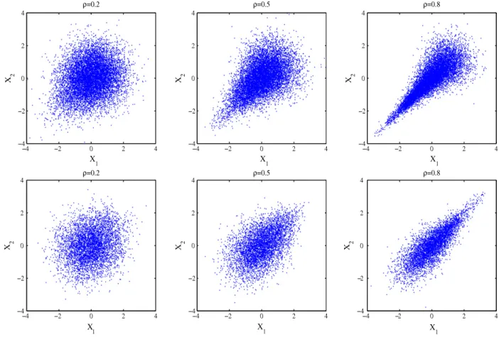
Fig. 2. Examples of bivariate input models with standard normal marginals and positive tail dependencies.

distribution [26]. Specifically, the positive lower-tail dependence

ν

L

(

i

,

j

)

between random variables Xi and Xj is the amount of dependence in the lower-quadrant tail of the joint distribution of Xi and Xjand thus, it is given by limℓ↓0Pr

(

Xi

≤

Fi−1

(ℓ)|

Xj

≤

F_j−1

(ℓ))

. The positive upper-tail dependence

ν

U

(

i

,

j

)

is, on the other hand, the amount of dependence in the upper-quadrant tail of the joint distribution of Xi and Xjand thus, it is given by lim_ℓ↑1Pr

(

Xi

≥

Fi−1

(ℓ)|

Xj

≥

Fj−1

(ℓ))

.Fig. 2provides examples of dependence structures for bivariate input models with standard normal marginals, but different positive tail dependencies [27]. The plots of the first, second, and third columns of this illustration are obtained for product-moment correlations of 0.2, 0.5, and 0.8, respectively. However, the first-row (second-row) plots exhibit greater dependence in the joint lower (upper) tail than in the joint upper (lower) tail; i.e.,

ν

L

(

i

,

j

) >

0 and

ν

U

(

i

,

j

) =

0 (

ν

U

(

i

,

j

) >

0 and

ν

L

(

i

,

j

) =

0). More specifically, the first-row (second-row) plots are obtained from a Clayton (Gumbel) distribution with parameters 0.43 (1.18) for the first column, 1.00 (1.71) for the second column, and 3.11 (3.80) for the third column (Section2). The plots of Fig. 2 also coincide with the plots of Burr–Pareto-Logistic family proposed by Cook and Johnson [28,29]. However, most multivariate input models, including the multivariate normal distribution [30], multivariate Johnson translation system [31], and the Normal-To-Anything (NORTA) distribution [32], measure the dependence between simulation inputs using correlation; therefore, they fail to capture the types of dependence structures illustrated inFig. 2.

The need for input models with asymmetric dependence struc-tures arises in situations where extreme positive realizations have a tendency to occur together. For example, Fortin and Kuzmics [33] show that the stock-return pairs of financial markets exhibit high dependence in the lower tail as well as low dependence in the upper tail of their joint distribution. Similar empirical evidence

for the need to measure tail dependence is provided in [34–36]. Patton [13], on the other hand, studies the dependence between mark–dollar and Yen–dollar exchange rates and shows that they are more dependent when they are depreciating than when they are appreciating. Thus, the asymmetric dependence structure of these exchange-rate processes cannot be adequately modeled by the widely used multivariate input models of the simulation input-modeling literature.

Despite our focus on copula-based input models represent-ing positive tail dependencies, it is important to note that the notion of negative tail dependence has been introduced by Zhang [37]. Specifically, the negative upper-tail dependence, which is called the lower–upper tail dependence in [37], is defined by lim_ℓ↓0Pr

(

Xi

≤

Fi−1

(ℓ)|

Xj

≥

Fj−1

(ℓ))

, while the negative lower-tail dependence, which is also known as the upper–lower lower-tail de-pendence, is given by lim_ℓ↑1Pr

(

Xi

≥

Fi−1

(ℓ)|

Xj

≤

Fj−1

(ℓ))

. Copula theory reviewed in this paper for positive tail dependence read-ily extends to these definitions of negative tail dependence. How-ever, most of the available empirical evidence has been for positive tail dependence. Although Sun and Wu [38] provide empirical ev-idence for the existence of negative tail dependence between the returns of the S&P 500 index and the returns of the Market Volatil-ity Index, the negative tail dependence is rarely mentioned. There-fore, we restrict the focus of this survey to the representation of positive tail dependence. In the next section, we describe how to utilize copula theory to develop multivariate input models with the ability to capture asymmetric dependence structures, which are characterized by the positive tail dependencies among the simu-lation input random variables.

3. Copula-based input modeling

Copulas have been used extensively for a variety of financial applications including Value-at-Risk calculations [39–41], option

pricing [42–46], credit risk modeling [47,48], and portfolio opti-mization [49,50]. For a comprehensive review of the applications of copulas in finance, we refer the reader to Patton [51]. However, copulas are not used only for solving financial problems; they are also used for decision and risk analysis [52], aggregation of expert opinions [53], estimation of joint crop yield distributions [54], dis-ruptive event modeling in project management [55], analysis of accident precursors [56,57], and modeling travel behavior by ac-commodating self-selection effects [58]. Recently, copulas have also been used in marketing to model the purchase behavior of customers [25], and in operations management to model retailer demands [14], supplier defaults [15], and supply disruptions in supply chains [16]. We provide the basics of copula theory in

Sec-tion3.1, review bivariate copula models in Section3.2, and present

multivariate copula models with three or more component ran-dom variables in Section3.3.

3.1. Fundamentals of copula theory

A way of modeling the dependence among the components of a k-dimensional random vector that avoids the pitfalls of correlation is to use a k-dimensional copula [18, Definition 2.10.6]:

Definition 1. A k-dimensional copula is a function Ck

: [

0

,

1

]

k

→

[

0

,

1

]

with the following properties: (1) For every u

=

(

u1

,

u2

,

. . . ,

uk

)

in

[

0

,

1

]

k

,

Ck

(

u

) =

0 if at least one coordinate of u is 0; and if all coordinates of u are 1 except u_ℓ, then Ck

(

u

) =

uℓfor

ℓ =

1

,

2

, . . . ,

k. (2) For every a

=

(

a1

,

a2

, . . . ,

ak

)

and b

=

(

b1

,

b2

,

. . . ,

bk

)

in

[

0

,

1

]

ksuch that a

≤

b; i.e., aℓ

≤

bℓ

, ℓ =

1

,

2

, . . . ,

k, and for every k-box

[

a

,

b

]

; i.e.,

[

a1

,

b1

] × [

a2

,

b2

] × · · · × [

ak

,

bk

]

, the Ck-volume given by∆baCk

(

t

) =

∆bakk∆

bk−1 ak−1

· · ·

∆ b2 a2∆ b1 a1Ck

(

t

)

with ∆bℓ aℓCk

(

t

) =

Ck

(

t1

, . . . ,

tℓ−1

,

bℓ

,

tℓ+1

, . . . ,

tk

) −

Ck

(

t1

, . . . ,

tℓ−1

,

aℓ

,

t_ℓ+1

, . . . ,

tk

)

is

≥

0.

The first condition of this definition provides the lower bound on the joint distribution function and insures that the marginal dis-tributions of the copula are uniform. The second condition insures that the probability of observing a point in a k-box is nonnegative. Thus, a k-dimensional copula is simply a k-dimensional distribu-tion funcdistribu-tion with uniform marginals.

It is important to note that copulas are not the only means to obtain joint distribution functions from uniform marginals. There exist useful families of multivariate uniform distributions that could be the basis for multivariate input modeling: Multivariate Burr distribution [59], multivariate Pareto distribution [60], and multivariate logistic distribution [61] are essentially obtained by transforming uniform marginal distributions to arbitrary marginal distributions. Similarly, Plackett’s distribution [62] is obtained by transforming bivariate uniform marginal distributions to arbi-trary marginal distributions, while Morgenstern’s distribution [63] with uniform marginals is generalized to have arbitrary marginal distributions in [64]. We refer the reader to Chapter 9 and Chap-ter 10 of Johnson [65] for a detailed discussion on obtaining mul-tivariate distributions with arbitrary marginals from mulmul-tivariate uniform distributions. This survey, however, focuses on tail depen-dence and therefore, describes the use of copulas to obtain mul-tivariate distributions with arbitrary marginals and positive tail dependencies.

The use of a copula for representing the joint distribution of a random vector has been studied extensively for the last two decades [66,67,26,68,18]. The name ‘‘copula’’ emphasizes the manner in which a k-dimensional distribution function is ‘‘coupled’’ to its k (one-dimensional) marginal distributions; this property is formally stated in Sklar’s theorem [18, Theorem 2.10.9]:

Theorem 1. Let F be a k-dimensional distribution function with

marginals Fi

,

i

=

1

,

2

, . . . ,

k. Then, there exists a k-dimensional copula Cksuch that for all xi

,

i

=

1

,

2

, . . . ,

k in domain

ℜ

k, F

(

x1

,

x2

, . . . ,

xk

) =

Ck

(

F1

(

x1

),

F2

(

x2

), . . . ,

Fk

(

xk

)) .

If Fi

,

i

=

1

,

2

, . . . ,

k are all continuous, then Ckis unique; otherwise, C_kis uniquely determined on RanF₁

×

RanF₂

×· · ·×

RanF_k. Conversely, if Ckis a k-dimensional copula and Fi

,

i

=

1

,

2

, . . . ,

k are distribution functions, then the function F is a k-dimensional distribution function with marginals Fi

,

i

=

1

,

2

, . . . ,

k.

The major implication of this theorem is that copula Ckis the joint distribution function of Ui

≡

Fi

(

Xi

),

i

=

1

,

2

, . . . ,

k, where the random variables Ui

,

i

=

1

,

2

, . . . ,

k are the probability inte-gral transforms of Xi

,

i

=

1

,

2

, . . . ,

k. Thus, each of the random variables Ui

,

i

=

1

,

2

, . . . ,

k follows a uniform distribution in

[

0

,

1

]

, regardless of the distributions of the component random variables Xi

,

i

=

1

,

2

, . . . ,

k. Moreover, Ckcan be uniquely deter-mined when the marginal cdfs Fi

,

i

=

1

,

2

, . . . ,

k are all contin-uous. If the marginal cdfs Fi

,

i

=

1

,

2

, . . . ,

k are all discrete, then Ckis uniquely determined on RanF1

×

RanF2

× · · · ×

RanFk, where RanFiis the range of the cdf Fi. In any case, the copula Ckcaptures the dependence structure of the joint cdf F and it can be written as Ck

(

u1

,

u2

, . . . ,

uk

) =

F

(

F1−1

(

u1

),

F2−1

(

u2

), . . . ,

Fk−1

(

uk

))

, where F_i−1is the generalized inverse of the marginal cdf Fi[18, Corollary 2.10.10].

The practical premise of Sklar’s theorem in multivariate input modeling is that the joint distribution F can be constructed by choosing the marginal distributions Fi

,

i

=

1

,

2

, . . . ,

k and the copula density function ckseparately. More specifically, any joint probability density function (pdf) f can be written as a product of its marginal pdfs fi

,

i

=

1

,

2

, . . . ,

k and copula density function ck for differentiable cdfs Fi

,

i

=

1

,

2

, . . . ,

k and differentiable copula Ck; i.e., f

(

x1

,

x2

, . . . ,

xk

) =

ck



F1

(

x1

),

F2

(

x2

), . . . ,

Fk

(

xk

)



·

k



i=1 fi

(

xi

).

The marginal pdf fi is obtained from

∂

Fi

(

xi

)/∂

xi, while

∂

kCk

(

u1

,

u2

, . . . ,

uk

)/(∂

u1

∂

u2

· · ·

∂

uk

)

provides the k-dimensional copula density function ck, encoding all of the information about the de-pendencies among the random variables Xi

,

i

=

1

,

2

, . . . ,

k. Thus, cktakes the value of 1 when Xi

,

i

=

1

,

2

, . . . ,

k are independent, and the joint density function reduces to the product of only the marginal pdfs.

There are numerous parametric families of copulas proposed in the literature, emphasizing different distributional properties. In this survey, we distinguish these copulas on the grounds of the tail dependence they capture; i.e., some copulas assign the value of zero to the tail dependence, while others represent positive lower-tail dependence and/or positive upper-lower-tail dependence. Next, we present a copula-based definition of the tail dependence for a bivariate input model with copula C2[26]:

Definition 2. If a two-dimensional copula C2is such that limu↓0C2

(

u

,

u

)/

u

=

ν

_L exists, then C2has lower-tail dependence if

ν

L

∈

(

0

,

1

]

and no lower-tail dependence if

ν

L

=

0. Similarly, if limu↑1

(

1

−

2u

+

C2

(

u

,

u

))/(

1

−

u

) = ν

Uexists, then C2has upper-tail

dependence if

ν

U

∈

(

0

,

1

]

and no upper-tail dependence if

ν

U

=

0. A close look at the existing literature reveals that one of the widely used copulas for bivariate input modeling is the

two-dimensional normal distribution. The application of

Def-inition 2 with the two-dimensional copula C2 replaced by

the two-dimensional standard normal cdf having correlation

ρ(

1

,

2

) ∈ (−

1

,

1

)

between random variables Z1

(≡

Φ−1

(

F1

(

X1

)))

Table 1

Bivariate copulas and their tail-dependence functions.

Copula Parameter νL νU Elliptically symmetric Normal −1< ρ <1 0 0 t −1< ρ <1,0<d< ∞ 2td+1 _{(d+1)(1−ρ)} (1+ρ)  2td+1 _{(d+1)(1−ρ)} (1+ρ)  Archimedean Clayton θ ≥0 2−1/θ ₀ Gumbel θ ≥1 0 2−21/θ θ ≥1 2−1/θ ₂₋₂1/θ θ1>0, θ2≥1 2−1/(θ1θ2) 2−21/θ2 Max-infinitely divisible θ1≥0, θ2≥1 2−1/θ1 2−21/θ2

the lower-tail dependence (

ν

L

(

1

,

2

) =

0) and the upper-tail de-pendence (

ν

U

(

1

,

2

) =

0) between random variables X1and X2.

Thus, regardless of the correlation

ρ(

1

,

2

) ∈ (−

1

,

1

)

we choose, extreme events appear to occur independently in X1and X2when

we go far enough into the tails. This explains why a bivariate input model building on the normal distribution fails to represent posi-tive tail dependencies.

This discussion readily extends to the multi-dimensional set-ting with k

≥

2. A well known multivariate input model building also on the normal distribution is the NORTA random vector in-troduced by Cario and Nelson [32]. The goal of this input model is to match the pre-specified properties of the random vector X

=

(

X1

,

X2

, . . . ,

Xk

)

′, i.e., the marginal distributions Fi

,

i

=

1

,

2

, . . . ,

k and the input correlations

ρ

X

(

i

,

j

),

i

,

j

=

1

,

2

, . . . ,

k, so as to drive

the simulation with random vectors that have these properties. Therefore, the construction of the NORTA random vector builds on (1) applying the probability integral transform Fito the input random variable Xi, which results in the uniform random variable Ui(i.e., Fi

(

Xi

) =

Ui); and (2) applying the inverse cdfΦ−1 to Ui from which the standard normal random variable Zi is obtained (i.e., Zi

=

Φ−1

(

Fi

(

Xi

))

). Consequently, we obtain the joint cdf F of the NORTA random vector X as follows:

F

(

x1

,

x2

, . . . ,

xk

)

=

Pr

(

Xi

≤

xi

;

i

=

1

,

2

, . . . ,

k

)

=

Pr

(

Fi

(

Xi

) ≤

Fi

(

xi

);

i

=

1

,

2

, . . . ,

k

)

=

Pr

(

Ui

≤

ui

;

i

=

1

,

2

, . . . ,

k

)

=

Pr



Φ−1

₍

_U i

) ≤

Φ−1

(

ui

);

i

=

1

,

2

, . . . ,

k



=

Pr



Zi

≤

Φ−1

(

ui

);

i

=

1

,

2

, . . . ,

k



=

Φ_k



Φ−1

₍

_u 1

),

Φ−1

(

u2

), . . . ,

Φ−1

(

uk

);

6k



=

Φ_k



Φ−1

(

F1

(

x1

)),

Φ−1

(

F2

(

x2

)), . . . ,

Φ−1

(

Fk

(

xk

));

6k



.

In this representation,Φk

(·;

6k

)

is the joint cdf of the standard normal random vector Z

=

(

Z1

,

Z2

, . . . ,

Zk

)

′with the correlation matrix 6k

≡ [

ρ(

i

,

j

);

i

,

j

=

1

,

2

, . . . ,

k

]

, where

ρ(

i

,

j

)

is the correlation between the random variables Ziand Zj. The function

Φk

(·;

6k

)

, which is simply the k-dimensional normal copula, cou-ples the arbitrary marginal cdfs Fi

,

i

=

1

,

2

, . . . ,

k with the cor-relation matrix6kto obtain the joint distribution function F . Thus, the dependence structure of the k-dimensional NORTA distribution is represented by the k-dimensional normal copula, explaining the failure of the NORTA distribution to represent non-zero tail depen-dencies. This result further extends to the multivariate normal dis-tribution and the multivariate Johnson translation system, which are the special cases of the NORTA distribution. Specifically, we ob-tain the multivariate normal distribution by allowing each of the NORTA components to have a univariate normal distribution; we obtain the multivariate Johnson translation system by letting each component of the NORTA random vector have a univariate Johnson distribution [69].

A solution to the problem of capturing asymmetric dependence structures with positive tail dependencies is to replace the k-dimensional normal copula of the NORTA random vector X with a

k-dimensional copula having the ability to match the pre-specified values of lower-tail dependencies

ν

L

(

i

,

j

),

i

,

j

=

1

,

2

, . . . ,

k and upper-tail dependencies

ν

U

(

i

,

j

),

i

,

j

=

1

,

2

, . . . ,

k. Section3.2 re-views the bivariate copula models that can be used for this purpose along with their tail dependence properties (i.e., k

=

2). Focusing on random vectors with three or more components (i.e., k

≥

3), Section3.3considers the representation of tail dependencies by multivariate input models.

3.2. Bivariate copula models

The existing literature contains numerous parametric families of bivariate copulas, emphasizing different distributional proper-ties [26,68,18]. In this survey, we consider the property of tail de-pendence.Table 1provides the bivariate copulas that can be used for capturing this measure of dependence between any pair of ran-dom variables.

3.2.1. Elliptically symmetric copulas

Both the normal copula and the t copula fall into the class of elliptically symmetric copulas, which are introduced in [70] and discussed comprehensively in [71] as the generalizations of the normal copula to those with elliptically symmetric contours. Thus, the elliptically symmetric copulas inherit many of the tractable properties of the normal copula and maintain the advantage of being easy to sample. Specifically, the bivariate normal copula with the dependence parameter

ρ ∈ (−

1

,

1

)

is given by

C2

(

u1

,

u2

;

ρ) =



Φ−1(u1) −∞



Φ−1(u2) −∞ 1 2

π

1

−

ρ

2

×

exp



−

z 2 1

−

2

ρ

z1z2

+

z22 2

(

1

−

ρ

2

)



dz1dz2

,

while the bivariate t copula with the degrees of freedom d

∈

(

0

, ∞)

is given by C2

(

u1

,

u2

;

ρ,

d

) =



t_d−1(u1) −∞



t_d−1(u2) −∞ 1 2

π

1

−

ρ

2

×



1

+

z 2 1

−

2

ρ

z1z2

+

z22 d

(

1

−

ρ

2

)



−(d+2)/2 dz1dz2

,

where the parameter

ρ

corresponds to a dependence parameter

when d

>

2. An important distinction between these two cop-ulas is that the normal copula assigns the value of zero to the tail dependencies, while both the lower-tail dependence and the upper-tail dependence captured by the t copula are given by 2td+1

(

√

d

+

1

√

1

−

ρ/

√

1

+

ρ)

, where tddenotes the univariate t distribution function with d degrees of freedom [23]. Thus, the t copula assumes positive tail dependence even for

ρ =

0, but the symmetry in the dependence structure (i.e., the equivalence be-tween the lower-tail dependence and the upper-tail dependence) restricts its use for bivariate input modeling; i.e., a property that is shared by all elliptically symmetric copulas.

3.2.2. Archimedean copulas

A family of non-elliptical copulas with the ability to capture asymmetric dependence structures (i.e., different values for lower-tail and upper-lower-tail dependencies) is the class of Archimedean copu-las. These copulas are analytically tractable in the sense that many of their properties can be derived using elementary calculus [66]. Specifically, an Archimedean copula with parameter

θ

is of the form C2

(

u1

,

u2

;

θ) = φ

−1

(φ(

u1

;

θ)+φ(

u2

;

θ); θ)

, where

φ

−1

(·; θ)

is the pseudo-inverse of

φ(·; θ) : [

0

,

1

] → [

0

, ∞]

, which is a continuous, strictly decreasing, and convex generator function satisfying

φ(

1

;

θ) =

0. Different generator functions lead to dif-ferent types of Archimedean copulas. For instance, the generator

φ(

t

;

θ) = (

t−θ

₋

₁

_)/θ

_{produces the Clayton copula C}

2

(

u1

,

u2

;

θ) =

(

u−₁θ

+

u−₂θ

−

1

)

−1/θ_{with 0}

_≤

_{θ < ∞}

_{, leading to a lower-tail}

de-pendence of

ν

L

(

1

,

2

) =

2−1/θ between random variables X1and

X2[72]. This is the copula function used for obtaining the first-row

plots ofFig. 2, while the second-row plots are obtained from the generator function

φ(

t

;

θ) = (−

log t

)

θ, which leads to the Gum-bel copula C2

(

u1

,

u2

;

θ) =

exp

(−((−

log u1

)

θ

+

(−

log u2

)

θ

)

1/θ

),

1

≤

θ < ∞

with an upper-tail dependence of

ν

U

(

1

,

2

) =

2

−

21/θ _{[73]. Thus, neither the Clayton copula nor the Gumbel}

cop-ula can simultaneously represent positive lower-tail and upper-tail dependencies. The generator function defined as

φ(

t

;

θ) =

(

t−1

−

1

)

θ, however, captures both the lower-tail dependence and the upper-tail dependence. More specifically, it produces the cop-ula C2

(

u1

,

u2

;

θ) = (

1

+

((

u−11

−

1

)

θ

+

(

u

−1

2

−

1

)

θ

)

1/θ

)

−1_with

θ ≥

1, leading to a lower-tail dependence of

ν

L

(

1

,

2

) =

2−1/θand an upper-tail dependence of

ν

U

(

1

,

2

) =

2

−

21/θ [18]. However, the values

ν

L

(

1

,

2

)

and

ν

U

(

1

,

2

)

can take are limited by the copula parameter

θ

.

A way to overcome this limitation of a single-parameter cop-ula is to construct a two-parameter Archimedean copcop-ula. This can be done by using a composite generator function of the form

φ(

t

;

θ

₁

, θ

₂

) = (φ(

tθ1

))

θ2_{. For example, defining the composite} generator function

φ(

t

;

θ

₁

, θ

₂

)

as

(

t−θ1

₋

₁

)

θ2_with

θ

1

>

0 and

θ

2

≥

1 leads to the two-parameter Archimedean copula C2

(

u1

,

u2

;

θ) =

(((

uθ1

1

−

1

)

θ2

+

(

u

θ1

2

−

1

)

θ2

)

1/θ1

+

1

)

−1/θ1 _{with a lower-tail} de-pendence of

ν

L

(

1

,

2

) =

2−1/(θ1θ2)and an upper-tail dependence of

ν

U

(

1

,

2

) =

2

−

21/θ2. The upper-tail dependence

ν

U

(

1

,

2

)

can take any value between 0 and 1, providing more flexibility than the single-parameter Archimedean copula in modeling the amount of dependence in the upper-quadrant tail of the underlying joint dis-tribution function. However, the value the lower-tail dependence

ν

L

(

1

,

2

)

can assume is restricted by the value of the upper-tail de-pendence

ν

U

(

1

,

2

)

. This modeling challenge is overcome by the max-infinitely divisible copulas introduced in the next section. 3.2.3. Max-infinitely divisible copulas

The lower-tail dependence

ν

L

(

1

,

2

) ∈ (

0

,

1

]

and the upper-tail dependence

ν

U

(

1

,

2

) ∈ (

0

,

1

]

between random variables X1

and X2can be jointly represented by using a family of copulas of

the form C2

(

u1

,

u2

) =

Θ

(−

log K

(

e−Θ −1_(u

1)

,

_e−Θ−1(u2)

))

_{, where}

Θis a Laplace transformation and K is a max-infinitely divisible bivariate copula between random variables U1

=

F1

(

X1

)

and

U2

=

F2

(

X2

)

. Specifically, the distribution function K is

max-infinitely divisible if Kαis a distribution function for every

α >

0 [74]. Furthermore, if K is an Archimedean copula, then C2

is an Archimedean copula. For example, letting K be the

one-parameter Clayton copula with one-parameter

θ

1

≥

0 and allowing

Θto be the Laplace transformation satisfyingΘ

(

t

) =

1

−

(

1

−

e−t

)

1/θ2 _{with parameter}

θ

2

≥

1 results in the two-parameter

copula of the form C2

(

u1

,

u2

;

θ

1

, θ

2

) = φ

−1

(φ(

u1

;

θ

1

, θ

2

) +

φ(

u2

;

θ

1

, θ

2

); θ

1

, θ

2

)

, where

φ(

t

;

θ

1

, θ

2

) = (

1

−

(

1

−

t

)

θ2

)

−θ1

−

1 [26]. The application ofDefinition 2to this copula function results

in the lower-tail dependence

ν

L

(

1

,

2

) =

2−1/θ1 and the upper-tail dependence

ν

U

(

1

,

2

) =

2

−

21/θ2. Thus, parameter

θ

1 (

θ

2)

is used only for adjusting the lower-tail (upper-tail) dependence

ν

L

(

1

,

2

) (ν

U

(

1

,

2

))

; i.e., the use of this two-parameter Archimedean copula for bivariate input modeling allows both the lower-tail dependence and the upper-tail dependence to assume arbitrary values in

[

0

,

1

]

. Further discussion on two-parameter bivariate copulas can be found in [26].

3.3. Multivariate copula models

In this section, we discuss the extension of the bivariate

cop-ula models presented in Section 3.2 to three or more random

variables. Specifically, Section3.3.1reviews the multivariate ellip-tical copulas; Section3.3.2presents the exchangeable multivari-ate Archimedean copulas; Section3.3.3provides the mixtures of max-infinitely divisible copulas; and finally Section3.3.4reviews the vine specifications that are known to be the most flexible mul-tivariate copula models with the ability to represent asymmetric dependence structures with positive tail dependencies.

3.3.1. Multivariate elliptical copulas

Two widely used copulas for representing the joint distribution of three or more input random variables are the normal copula associated with the multivariate normal distribution and the t copula associated with the multivariate t distribution. Each of these copulas is a member of the elliptical copula family that is particularly easy to use for driving stochastic simulations with multiple inputs. Specifically, the multivariate normal copula with the positive definite correlation matrix6k

≡ [

ρ(

i

,

j

);

i

,

j

=

1

,

2

,

. . . ,

k

]

is given by Ck

(

u1

,

u2

, . . . ,

uk

;

6k

)

=

Φ_k



Φ−1

₍

_u 1

),

Φ−1

(

u2

), . . . ,

Φ−1

(

uk

);

6k



,

=



Φ−1(u1) −∞

. . .



Φ −1_(u k) −∞ 1

(

2

π)

k/2

_|

₆ k

|

1/2

×

exp



−

1 2z ′₆−1 k z



dz1

. . .

dzk

,

where z denotes the vector

(

z1

,

z2

, . . . ,

zk

)

′. The limitation of this multivariate copula in representing positive tail dependence becomes apparent in modeling investor’s default risk [75,76]. For further discussion on the limitations of the multivariate normal copula, we refer the reader to Lipton and Rennie [77], Donnelly and Embrechts [78] and Brigo et al. [79].

The multivariate t copula with the parameters6k

≡ [

ρ(

i

,

j

);

i

,

j

=

1

,

2

, . . . ,

k

]

and d

∈

(

0

, ∞)

is given by Ck

(

u1

,

u2

, . . . ,

uk

;

6k

,

d

)

=

t



t_d−1

(

u1

),

td−1

(

u2

), . . . ,

td−1

(

uk

);

6k

,

d



,

=



t_d−1(u1) −∞

. . .



t−_d1(uk) −∞ Γ



_d+k 2

 |

6k

|

−1/2 Γ



_d 2



(

d

π)

k/2

×



1

+

1 dz ′₆−1 k z



−d+₂k dz1

. . .

dzk

.

Even for

ρ(

i

,

j

) =

0, the multivariate t copula represents sym-metric tail dependencies

ν

L

(

i

,

j

) = ν

U

(

i

,

j

) =

2td+1

(−

√

d

+

1

√

1

−

ρ(

i

,

j

)/

√

1

+

ρ(

i

,

j

))

, as can be deduced fromTable 1by fo-cusing on the interaction between random variables Xi and Xj. Thus, the multivariate t copula fails to capture asymmetric depen-dence structures with different values for lower-tail and upper-tail dependencies. In the following section, this limitation of the multivariate t copula is overcome by using the exchangeable Archimedean copula for multivariate input modeling.

We conclude this section by noting that the class of the ellipti-cally symmetric copulas includes the logistic copula [71], the ex-ponential power copula [80], and the generalized t copula [81,82]. However, not all generalized t copulas are elliptically symmetric; they allow for different degrees of freedom and different types of dependencies among the components of the random vector. We refer the reader to Mendes and Arslan [82] for the characterization of the tail dependencies that can be captured by the generalized t copulas.

3.3.2. Exchangeable multivariate Archimedean copulas

The extension of the Archimedean copula introduced in

Section 3.2 for bivariate input modeling is the k-dimensional

Archimedean copula of the following form: Ck

(

u1

,

u2

, . . . ,

uk

;

θ)

=

φ

−1

(φ(

u1

;

θ) + φ(

u2

;

θ) + · · · + φ(

uk

;

θ); θ) .

φ(·; θ) : [

0

,

1

] → [

0

, ∞)

is a continuous, strictly decreasing function that satisfies

φ(

0

;

θ) = ∞

and

φ(

1

;

θ) =

0. Additionally,

φ

−1

_{(·; θ)}

_{is a completely monotonic function on}

_[

₀

_{, ∞)}

_(i.e.,

(−

1

)

ℓ

∂

ℓ

φ

−1

(

t

;

θ)/∂

tℓ

≥

0 for all t

∈

(

0

, ∞)

and

ℓ =

0

,

1

,

. . . , ∞

) [83]. This is a necessary and sufficient condition for the function Ck

(·; θ)

to define a copula, and this condition is satisfied by both the k-dimensional Clayton copula and the k-dimensional Gumbel copula.

Specifically, the pseudo-inverse of the generator function of the Clayton copula; i.e.,

φ

−1

(

t

;

θ) = (

1

+

t

)

−1/θ is completely monotonic on

[

0

, ∞)

. Therefore, the k-dimensional Clayton copula with

θ >

0 is given by Ck

(

u1

,

u2

, . . . ,

uk

;

θ) = 

u −θ 1

+

u −θ 2

+ · · · +

u −θ k

−

k

+

1



−1/θ

.

Due to its ability to represent the joint probability of compo-nent random variables taking very small values together, Tehrani et al. [16] use this copula function to model dependent disruptions in supply chains caused by catastrophic events. Wagner et al. [15], on the other hand, use the multivariate Clayton copula for inves-tigating the impact of positive default dependencies on the de-sign of supplier portfolios. However, the k-dimensional Clayton copula assumes a lower-tail dependence of 2−1/θ _{and an}

upper-tail dependence of zero between all pairs of its components (i.e.,

ν

L

(

i

,

j

) =

2−1/θand

ν

U

(

i

,

j

) =

0 for i

=

1

,

2

, . . . ,

k and j

=

i

,

i

+

1

,

. . . ,

k), limiting its ability to perform flexible dependence model-ing.

Similarly, the pseudo-inverse of the generator function of the Gumbel copula; i.e.,

φ

−1

₍

_t

_;

_{θ) =}

_exp

₍₋

_t1/θ

₎

_{is completely}

mono-tonic on

[

0

, ∞)

. Thus, the two-dimensional Gumbel copula of Sec-tion3.2is generalized to the following k-dimensional copula with

θ ≥

1:

Ck

(

u1

,

u2

, . . . ,

uk

;

θ)

=

exp



−



(−

log u1

)

θ

+

(−

log u2

)

θ

+ · · · +

(−

log uk

)

θ



1/θ

 .

The functional form of this copula leads to the tail dependencies of

ν

L

(

i

,

j

) =

0 and

ν

U

(

i

,

j

) =

2

−

21/θ for i

=

1

,

2

, . . . ,

k and j

=

i

,

i

+

1

, . . . ,

k.

The bivariate two-parameter Archimedean copulas can also be generalized to be the k-dimensional Archimedean copulas. As an example, we consider the composite generator function

φ(

t

;

θ

₁

, θ

₂

) = (

t−θ1

₋

₁

)

θ2 _with

θ

1

>

0 and

θ

2

≥

1. Since the

pseudo-inverse of this generator function is completely monotonic on

[

0

, ∞)

, we obtain the following k-dimensional copula:

Ck(u1,u2, . . . ,uk;θ1, θ2) =  (u−θ1 1 −1)θ2+(u −_θ1 2 −1)θ2+ · · · +(u −_θ1 k −1)θ2 1/θ2 +1 −1/θ1 . Therefore, the tail dependencies

ν

L

(

i

,

j

)

and

ν

U

(

i

,

j

)

are, respec-tively, identified as 2−1/(θ1θ2)_{and 2}

₋

₂1/θ2_{for i}

₌

₁

,

₂

, . . . ,

_{k and} j

=

i

,

i

+

1

, . . . ,

k.

3.3.3. Mixtures of max-infinitely divisible copulas

A flexible bivariate copula with the ability to represent any pair of lower-tail and upper-tail dependencies is the max-infinitely divisible bivariate copula (Section3.2). Thus, a natural question to ask is whether it is possible to build on the mixtures of max-infinitely divisible bivariate copulas so as to construct a k-dimensional copula that would match arbitrary values of

ν

L

(

i

,

j

) >

0 and

ν

U

(

i

,

j

) >

0 for i

=

1

,

2

, . . . ,

k and j

=

i

,

i

+

1

,

. . . ,

k. While the answer to this question is no, there exists a multivariate copula function, Ck

(

F1

(

x1

),

F2

(

x2

), . . . ,

Fk

(

xk

))

from the family of extreme value copulas, which captures arbitrary values for the positive upper-tail dependencies among the random variables X₁

,

X₂

, . . . ,

X_k, while modeling the positive lower-tail dependencies with limited flexibility:

Θ



−

k



i=1 k



j>i log Ki,j

(

e−Θ −1_(F i(xi))/(ϑi+k−1)

,

e−Θ−1(Fj(xj))/(ϑj+k−1)

) +

k



i=1

ϑ

i

ϑ

i

+

k

−

1 Θ−1

₍

_F i

(

xi

))



.

For this representation, Joe [26] provides the interpretation that

Laplace transformation Θ represents a minimal level of

pair-wise global dependence, bivariate copula Ki,jadds individual pair-wise dependence beyond the global dependence, and parameters

ϑ

i

,

i

=

1

,

2

, . . . ,

k lead to bivariate and multivariate asymme-try. Usually, the

ϑ

i

,

i

=

1

,

2

, . . . ,

k are nonnegative, although they can be negative if some of the copulas Ki,jcorrespond to inde-pendence. What is important to recognize here is that the Laplace transformationΘ limits our ability to represent arbitrary values for

ν

L

(

i

,

j

) >

0 and

ν

U

(

i

,

j

) >

0. This can be shown by selecting the Galambos copula for Ki,j; i.e.,

Ki,j

(

ui

,

uj

;

θ

i,j

)

=

uiujexp





(−

log ui

)

−_θi,j

₊

(−

_{log u} j

)

−_θi,j



−1/θi,j



with 0

≤

θ

_i,j

< ∞

[84], and by choosing the Laplace transforma-tionΘas gamma type; i.e.,Θ

(

s

) = (

1

+

s

)

−1/δ with parameter

δ ≥

0. In this case, we obtain an upper-tail dependence of

ν

U

(

i

,

j

) =

(ϑ

i

+

k

−

1

)

θi,j

+



ϑ

j

+

k

−

1



θi,j



−1/θi,j

and a lower-tail dependence of

ν

L

(

i

,

j

) =



2

−

(ϑ

_i

+

k

−

1

)

θi,j

₊



ϑ

j

+

k

−

1



θi,j



−1/θi,j



−1/δ

for i

=

1

,

2

, . . . ,

k and j

=

i

,

i

+

1

, . . . ,

k. The parameter

θ

i,j is specific to the joint distribution of random variables Xi and Xj, while global parameter

δ

is shared among all k components Xi

,

i

=

1

,

2

, . . . ,

k. Therefore, we can represent any arbitrary value of upper-tail dependence between any pair of component random variables, but the global parameter

δ

limits our ability to have the same level of flexibility in representing lower-tail dependence.

To conclude, the use of mixtures of max-infinitely divisible copulas as well as multivariate Archimedean copulas for input modeling allows the representation of both the lower-tail depen-dence and the upper-tail dependepen-dence among the components of the random vector. However, the dependence structures captured by these copula families are restricted by the use of insufficient number of copula parameters. Although this particular limitation is overcome by the vine copula we present in the following section, the copula-vine method characterizes the dependence structure of the random vector using a mix of bivariate tail dependencies and bivariate conditional tail dependencies. Thus, in low-dimensional settings the simulation practitioner, who is interested in generat-ing random vectors with pre-specified (unconditional) pair-wise

lower-tail and upper-tail dependencies, might find the use of the mixtures of max-infinitely divisible copulas of this section more convenient than the vines of the following section.

3.3.4. Vines

A vine is a graphical model introduced in [85], studied extensively in [86–89], and described comprehensively in [90] for constructing multivariate distributions using a mix of bivariate and conditional bivariate distributions of uniform random variables. Specifically, a k-dimensional vine is a nested set of k

−

1 spanning trees where the edges of tree j are the nodes of tree j

+

1, starting with a tree on a graph whose nodes are the k component random variables Xi

,

i

=

1

,

2

, . . . ,

k. A regular vine is, on the other hand, a vine in which two edges in tree j are joined by an edge in tree j

+

1 only if they share a common node [90, Section 4.4].

Fig. 3presents a four-dimensional vine, which is a nested set

of three spanning trees. Specifically, the first tree of this regular vine is the collection of three bivariate distributions; i.e., the joint distribution of the component random variables X1and X2,

the joint distribution of X2 and X3, and the joint distribution of

X3 and X4. Since the solid line between X1 and X2 links these

random variables, we associate this solid line with the joint distribution of X1 and X2, and label it as ‘‘1, 2’’, implying the

copula density function c2

(

F1

(

x1

),

F2

(

x2

))

. Similarly, we denote

the solid line between X2 and X3 by ‘‘2, 3’’ associated with the

copula density function c2

(

F2

(

x2

),

F3

(

x3

))

, and use ‘‘3, 4’’ for the line

between X3 and X4to correspond to the copula density function

c2

(

F3

(

x3

),

F4

(

x4

))

. The second tree, on the other hand, contains

two bivariate distributions, which are the joint distribution of X1

|

X2and X3

|

X2and the joint distribution of X2

|

X3and X4

|

X3with

the respective copula density functions c2

(

F1|2

(

x1

|

x2

),

F3|2

(

x3

|

x2

))

and c2

(

F2|3

(

x2

|

x3

),

F4|3

(

x4

|

x3

))

. Therefore, inFig. 3we mark the

lines ‘‘. . . ’’ of the second tree by ‘‘1

,

3

|

2’’ and ‘‘2

,

4

|

3’’. Finally, the third tree corresponds to the joint distribution of X1

|

X2

,

X3

and X4

|

X2

,

X3 represented by the line ‘‘–..–’’, which is further

labeled by ‘‘1

,

4

|

2

,

3’’ implying the copula density function c2

(

F1|2,3

(

x1

|

x2

,

x3

),

F4|2,3

(

x4

|

x2

,

x3

))

.

The two edges of a tree inFig. 3are joined only if they share a common component random variable to obtain an edge of the following tree. For example, the edges ‘‘1, 2’’ and ‘‘2, 3’’ of the first tree share the node associated with the random variable X2

and they are combined for the edge ‘‘1

,

3

|

2’’ of the second tree, while the edge ‘‘2

,

4

|

3’’ of the second tree is obtained from the edges ‘‘2

,

3’’ and ‘‘3

,

4’’ sharing the node of the random variable X3.

Similarly, the edges ‘‘1

,

3

|

2’’ and ‘‘2

,

4

|

3’’, which share the nodes associated with the random variables X2and X3in the second tree,

are joined by the edge ‘‘1

,

4

|

2

,

3’’ of the third tree in a manner that is consistent with the definition of a regular vine.

More specifically, the regular vine inFig. 3is known as the drawable vine (D-vine). Its use for multivariate input modeling allows the four-dimensional copula density function to be represented by the product of the six bivariate linking copulas illustrated inFig. 3; i.e.,

c4

(

F1

(

x1

),

F2

(

x2

),

F3

(

x3

),

F4

(

x4

))

=

c2

(

F1

(

x1

),

F2

(

x2

)) ×

c2

(

F2

(

x2

),

F3

(

x3

))

×

c2

(

F3

(

x3

),

F4

(

x4

)) ×

c2



F1|2

(

x1

|

x2

),

F3|2

(

x3

|

x2

)

×

c2



F2|3

(

x2

|

x3

),

F4|3

(

x4

|

x3

)

×

c2



F1|2,3

(

x1

|

x2

,

x3

),

F4|2,3

(

x4

|

x2

,

x3

) .

The bivariate linking copulas of the first row appear in the first tree of Fig. 3, while the bivariate linking copulas of the next two rows come from the second and third trees. Furthermore, this characterization of the four-dimensional random vector is easily generalized to a k-dimensional random vector; i.e., the joint

Fig. 3. AD-vine specification on four dependent random variables.

Fig. 4. AC-vine specification on four dependent random variables.

Fig. 5. An example of a non-regular vine on four dependent random variables.

density function of the k-dimensionalD-vine copula is obtained as a factorization of the univariate marginal density functions



k

i=1fi

(

xi

)

and the product of the bivariate (unconditional) linking copulas

k−1



i=1

c2

(

Fi

(

xi

),

Fi+1

(

xi+1

))

of the first tree and the bivariate (conditional) linking copulas k−1



j=2 k−j



i=1 c2

(

Fi|i+1,...,i+j−1

(

xi

|

xi+1

, . . . ,

xi+j−1

),

Fi+j|i+1,...,i+j−1

(

xi+j

|

xi+1

, . . . ,

xi+j−1

))

of the remaining k

−

2 trees. Representing the dependence

structure of the k-dimensional random vector via these

(

k

−

1

)(

k

−

2

)

bivariate copulas instead of a single k-dimensional copula leads to computational tractability in the development of data-fitting algorithms in Section 4, goodness-of-fit tests in Section 5, and sampling procedures in Section 6for copula-based multivariate input modeling.

Nevertheless, no unique regular vine exists for representing the dependence structure of a random vector.Fig. 4presents another type of four-dimensional regular vine, the canonical vine (C-vine), which is often used for multivariate input modeling. Fig. 5, on the other hand, provides an example of a four-dimensional non-regular vine. The comparison of this vine to the non-regular vines in

Figs. 3and4shows that the dependence structure of the regular

vine is represented in terms of unconditional and conditional dependence measures that are algebraically independent of each other; i.e., they do not need to satisfy any algebraic constraints for positive definiteness. Therefore, all assignments of the numbers between

−

1 and 1 to the edges of the regular vine are consistent