Ray representation for k-trees

Pattern Recognition Letters It) i [959) SIS—320 North-Holland

66

November [989

Ray representation for k-trees

Varol AKN‘IAN

Department of Computer Engineering and Informuitmi St‘it’nt'es. Biikuui L'niiersiii'. PO. Box a. ”6572 .Hailepe. Ankara.

Turkm-Wm. Randolph FRANKLIN

Department of Electrical, Computer. irrtdSi'xii-mi Engineering, Rem‘seiuer Pnii‘iet'hme Institute. Troy, NY 13130-3590. USA Received 25 March 1989

Abstract: k-trces ban: established themselves as useful data structures in pattern recognition. A fundamental operation regarding k-trees is the construction ota it-trce. We present a method to store an object as a set ol‘ rays and an algorithm to convert such a set into a k-tree. The algorithm is conceptually Simple. works for any A". and builds a k-tree from the rays very fast. It produces a minimal k-tree and does not lead to intermediate storage swell.

Key words: Hierarchical data structures, representation of rigid solids. rays. stacking.

1. Introduction

k-trees are data structures based on the symmet-ric recursive partitioning ol‘space. In order to make the upcoming presentation more concrete and the definitions less cumbersome. hereafter we shall

choose octrees (k = 3) as the representative member

of this group. It will be observed that our results will be applicable to both quadtrees (k = 2) and k-trees with k > 3 as well.

We are concerned in this paper with a task of fun damental importance in systems based on octrees. This is the operation of constructing an octree. The algorithms cited in recent overviews [1.2] are nei-ther efiicient nor conceptually easy to understand and implement.

We aim to accomplish two things: (i) propose a new way of storing an object as a set of rays. and (ii) describe an original algorithm to convert this set of rays into an octree. In a previous publication [3]. we have called the rays parallelepipeds. It will be seen that the latter term is indeed more suggestive but for the sake of conciseness we shall adopt the former.

0(67»8655 89 $3.50 © I989. Elsevier Science Publishers BN1 (North-Holland)

2. Termhobgy

An octree is a special case of the abstract data type digital s'i‘tit‘t‘ii tree [5]. The object. which we shall denote as “. is contained in a universe. I. which is a cube of size U x U x U where U = 2’.

Here I is a positive integer. 7' is made of U3 small

cubes of unit volume called iroxels. To obtain an oc-tree. which wc shall denote as Q. l’ is continuously subdivided into eight symmetric octants of equal volume. Each of these octants will either be homo‘ geneous (i.e.. either fully occupied by E or void) or heterogeneous tie. partly occupied by E). We fur-ther subdivide the heterogeneous octants into sub-octants, This is stopped when octants (possibly

voxels) of uniform properties are obtained.

Following the established usage. let us consider the obeis, An obel can be empty-Juli. or partial. l’ is considered to be a level-O obel. If E is not void but does not till 1’ either. then the universe obel is

labeled as partial. Then the following recursive

process is carried out. Iii < K then a partial obel at level-[ is divided evenly into eight obels at level i + I. Each of these obels is again labeledtiiil. empty.

\ olume it). Numberf

or partial and the process is repeated on the partial ones. Let us assume. without loss of generality. that the partial voxels. if any. at level-/' are arbitrarily declared to be full.

The level of an obel v in an oetree is detined re— cursively as let't'ltvi : t}. in ease \' is the root and as [ere-dirt = i'ei'eltiiitlit‘rii-ii + 1. otherwise. The depth ofan octree is understood as the level of its deepest

(lowest) leaf.

3. Relev ant research

Quadtrees. octrees. and to a lesser extent higher

dimensional lt-trees have proved to be a fertile area of research with many hundreds of papers and var-ious surveys. A recent. rather nontechnical over-view is provided by Samet and Webber [1.3] who cite about 300 references (althOugh with some im-portant omissions). Since we carry no pretensions of covering all the relevant work. we shall be selec-tive and refer the reader to Requicha [6} and Srihari [7] for two informative surveys on the representa-tion of rigid solids.

Early work on quadtree algorithms was done by

Hunter and Steiglitz [8} who showed how to per» form a set of operations on images using quadtrees. Jackins and Tanimoto [9] extended this work to oc-trees. Doctor and Torborg [l0] presented display techniques for octree-encoded objects.

Construction of a software system to represent and manipulate irregular 3D objects was first ac-complished by Meagher [1]]. His system lets the user build quadtrces interactively. extend them to

oetrees. and carry out transformations and

set-theoretic operations on them. Later. Meagher built a special hardware. ‘The Solids Engine'. which is a system for interactive solid modeling based on oc-trees.

Techniques for building octrees include merging the cross—sectional images (which are represented as quadtrees] of the object in sequence. This technique is examined by Yau and Srihari [l 2]; they show how to construct a k—dimensional tree representation from multiple (k — li-dimensional cross-sectional images. It is noted that there is a superficial resem-blance between the algorithm in [ll] and our algo-rithm. Tamminen and Samet [13] give an algorithm

3H1

PA TTFRN RECOL'JNITION LETTERS Nov ember l 95‘)

for converting from the boundary representation of a solid to the corresponding octree model using a technique called ‘eonnectivity labeling'. Samet [H] considers the conversion of tasters to quadtrees.

Sometimes. it is possible to use a small number of 2D images to reconstruct an octree representa-tion of a 3D object. This is done by taking silhou-ettes from various viewpoints. These silhousilhou-ettes are then proceSsed to create a bounding volume that serves as an approximation ol‘tlie object. cf. Potme-sil [15].

4. Ray representation

Ray representation has. in fact. been known for

a long time. For example. to compute the volume

of a 3D object. 5. one approximates it with a set of rectangular parallelepipeds. These parallelepipeds

(or. as noted before. rays. from now onl are as—

sumed. without loss of generality. to be evenly spaced in the xy—plane but to have varying lengths along the :fiirection. Figure 1 shows the rays for a JD object (region). In 3D these thin rectangles would become thin parallelepipeds. We assume throughout this paper that the rays are cast at unit spacing.

Let each ray be given in the format p 2

l.\'._l.'.:1.:;.’tl.tl:]. ‘~\:tct‘€ .\‘.}‘.:;.Z:E[O.U - I}. This

corresponds to a ray with fixed (Lt) that enters the object at :l and leaves it at :3 (assume that :l g :2). When an object is given as a set of rays. it is as— sumed that all rays in the set are distinct and dis-joint. The siujrttt'e normals iil and P1; are associated with :l and :1. respectively. They are used to dis-play E realistically so that the user can determine its shape. especially if it is an irregular object. In the sequel. we sometimes ignore the surface normals Since they can be easily handled by our algorithm.

E

tr:

Figure 1 Rd) representation for a region Iregion boundary not shown‘i,

Volume ll). Numbcri

There are several advantages ofthe ray format: ' Set—theoretic (Boolean) operations on two

oc-trees can be performed via trivial operations on rays since rays are 1D.

Translation of a ray is easy. (Rotation is still problematic.)

' To display an octree stored as a set of rays. we

simply paint the rays into the frame butler back to front. Notice that this would work for any display angle.

5. Rays from quadrie solids

Before we present our algorithm to build an oc-tree from a set of rays. we consider the problem of obtaining a ray representation for quadric solids. eg. an ellipsoid. Thus. we shall effectively show how to obtain an octree from a quadrie solid. since the output rays from the following process are direcly supplied as input to the stacking algorithm of Section 7. it is fair to note that quadric solids are

taken as an exemplary case for they are neither too trivial nor too complicated (like bieubic patchest.

The algorithm below was implemented in For-tran—T? on a Prime 750.

Let E be a 4 x 4 matrix and let 1 be the vector

[x y : l]". (The superscript T denotes the transpose.)

A concise way of writing down the equation of a quadric is then 1 "31' = 0. We first clip a quadric solid to the unit cube lie. [0. l]’) and then output a set of rays and surface normals as described be-fore. We assume that each ray goes through the lower left corner of the obel: the alternatiye would have been that the rays go through the center.

The algorithm to obtain rays from quadric solids is as follows:

Algorithm

0. lterate up the quadric solid in y. For each y. find the 3D conic in .\' and :.

I. For each conic in the x:-plane. find the range

of x for which : is real. This range contains up to

two (0. l. or 3) segments that may be finite or

inti-nite. To determine the range of x for which the 3D conic fuzz) is real. six cases should be considered

depending on the discriminant of the formal solu-tion for : in terms of x. That is. if f'lx.:) =

PATTERN RECOGNITION LETTERS N'm ember 1%“)

of + (ha — lilx): #— lcn + clx + cg“) = 0.

then

the discriminant is (its) : (hm + h; t)3 .. Jute... + t'1.\' + (33(2). The six cases are: nix) is always posi-tive; tilt) is positive outside a finite interval; til )5] is positive inside a finite interval; tilx) is nexer

posi-tive; tilxl is positive above a certain value; and

final-ly. nix) is positive below a certain Value,

2. lterate in x and solve the quadratic equation for :._ and :2. Clearly. they are clipped to [0, l].

3. Calculate the normals in the usual way. If :, were clipped in step 3. then the associated normals would be (0.0 i l).

The above algorithm is fast because it doesn‘t work with the rays that do not intersect the object. For reasonable objects. these are typically the ma-jority ofall the rays.

For ray tracing higher order solids. such as bi-cubic patches. we propose to use the following

ob-servation. The functions-tiny) and nlx._t') ._ for in—

tcrscctions and normals 7 although complicated. are smooth. Therefore. efficient simple approxima-tions using splines can be found.

6. Combining and splitting

Now we come to the main concern of the paper.

At the core of our algorithm for piling up an octree

are two operations: combining and splitting. We

now explain them. Given a ray

These are computed recursively as follows. First

search for the longest (in :) row in p and remote it

from p, This is a maximal row. Now p is either re-duced to a shorter ray or divided into two rays both shorter than the original. in both cases. the search continues until maximal rows of :-length equal to l are obtained. it is noted that. once the maximal rows of p are found. it should be impossible to ob-tain a longer row by putting two maximal rows

to-gether. For example. Figure 2 shows the nine maxi— mal rows obtained from the ray (l. 1.17.93).

A row at level-i is a triple l.\'._t',:l where : is divisi-ble by I” “. Clearly. this is shorthand for the ray

(.\'."t'.:.: ~.- 2’ ' ‘ i l); in other words. the :—length of

a row at level-i is always 2’

u. we need the maximal rows of p.

". Two rows. pi =

(xhrpn and u1 = l.\'3.y3.:). at the same leycl are

Volume 10. Numberj

length of row

' 2 4 B 32 15 a 4 I

it 3 :; .,_; m M 11.1

; ”in.

Figure 3. Splitting J ray (l. l. [7. L33) into nine maximal routs

mm) (L) the settle).

called adjacent if x. = x2 and l)‘. -— ‘1‘: = I. (Note

that they both have the same z.) A set of 2‘ rows at level K A i can be combined if. when sorted by y to get a set of rows. every row in this set is adjacent to its predecessor and its successor. When rows are combined one obtains squares which are explained below. _{For example. the rows (0.0.0). (0. LG).}

(0.3.0). and (0.3.0) at level / — l can be combined.

while the rows (0.1.0). (0.2.0). (0.3.0) and (0.4.0) at level / — I cannot (Figure 3).

Let pin-72.... be a set of Bi combinable rows at

level / — i. A square. 0. at level X A i is obtained by combining them into a single triple (x.y.:) where

x =p1's .t.:=p1‘s :. and y :min. p.75 _)'. Two

squares. a. =(x1.y.,:) and a; = (x3435) at the same level are called adjacent if y. = y; and x. — = l. A set of2i squares at level / —— {can be mm-bined if. when sorted by x to get a set of squares. every square in this set is adjacent to its predecessor

and its successor. As a result of combining squares

we obtain cubes which are defined below. For ex—

ample. the squares (0.0.0). (l.0.0). (2.0.0). and

(3.0.0) at level / —i are combinable while the .v; (0.3.0) (0.2.0) v; _(m C4) (0.1.0) (0.0.0) (0.4.0) . .A. . (0.3.0) fl .0 (0.2.0) (0.1.0)

Figure 3. Four rows of length four that are combined into one square versus four rows that cannot be combined. since they are

misaligned.

PATTERN RECOGNITION LETTERS November 1989

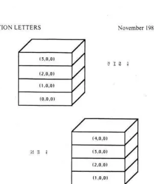
(4.0.0) iii 3'.) l (3.0.0) (2.0.0)

(1.0.0)

Figure 4. Four squares ot‘length four that are combined into one cube versus (our squares that cannot be combined. since they are

misaligned.

squares (|.0.0). (2.0.0). (3.0.0). and (4.0.0) are not

(Figure 4).

Let 01.02.... be.2‘ combinable squares at level .v‘ — i. A cube. K. is obtained as the triple (x._v.:) where y = a.‘s y.: 2 01‘s 2. and x = min.- a.‘s x.

If a row (,\‘.I)'.:) .:t level-i is split in the :

di-rection. then two rows. (x431) and (x.y.: +0).

are obtained at level 1+ l. [fa square (x.y.:) at level—i is split in x and y directions, then four squares. (.x‘.‘v.:). t.v.)'+ft.:). (.v+fi.y.:) and

(x «1- It.) ¢ h.:). are obtained at level 1-)- 1. Here

it = 2" ‘l'1.()bviously. the idea of splitting is gene-rizable to cubes and h} percubes. once we are at 2 4D. See Figure 5 for illustrations ol‘ splitting.

Figure 5. Two rows of length {out that cannot be combined into A square but can be split into ("our rows oflength two and

Volume 10. Numberi

The main data structure is a set of lists which will be called ittlists (dimension-level lists). An indi-vidual list in this set is denoted as JD_L. where D de-notes the dimension and L dede-notes the level it be-longs to.

7. The stacking algorithm

We assume that each ray has already been di-vided into its maximal rows and these maximal rows have already been inserted into the relevant lD std-lists.

Our stacking algorithm first tries to combine ad-jacent rows into squares. If a row cannot be com-bined, it will be split into two smaller (half-size) rows which are tried until the remaining pieces are at level—f. These are inserted into 9 since there is no way they can be combined.

Then the stacking algorithm tries to combine ad-jacent squares into cubes. Any square that cannot be thus combined will be split into four smaller (quarter-size) squares and the process will be re-peated until the remaining pieces are at level-K. These latter pieces are added to 9. Clearly. the ob— tained cubes are also added to £2. It is noted that the elements of inL are rows when l) = 1. squares when D = 2. cubes when D = 3. and hypercubes when D > 3. Our algorithm is still correct when D > 3 as a result of its general approach. Another important point to observe is that we need (k — l) x (f + l)lists in k-dimensional space.

This process will build the octree. Q. in its re— duced form. (An octree is in its reduced form if it has no partial nodes with all empty or all full children.)

When there are many rays. it may be suitable to use linear disk files to implement .H-lists. Only three files will be open during the execution of the stacking algorithm: (or. for read operations and [0+ LL and in“1 for write operations. Since the reads always take place sequentially and the writes are always carried out as appends, the algorithm is safe against virtual-memory page faults.

The algorithm works by iterating on dimensions as follows.

Algorithm

0. Each ray is partitioned into a set of rows which

PATTERN RECOGNITION LETTERS Nmember 1989

comprise a 1D octree. Thus. each row has a length which is a power of 2 and a starting : value which is a multiple ofits length.

l. The rows are sorted into lexicographic order by 0.2.x), This is necessary to detect combinablc rows in oneapass.

2. Adjacent rows are combined into squares whenever this is possible. A square has a side of 2’ for some 0 S l S ,f and starting x and : coordinates that are multiples of 2‘. If wefind 2‘ rows with posi~ tions

(i x 3‘ + m] x 11; x 2‘).

where m : 0...2‘. then we can combine them into one square. Combining rows is illustrated in Figure 3. The process of combining and splitting starts at l: O and iterates up to K. At any I. after all the rows that can be combined are indeed combined into squares. the remaining squares are each split into

two rows of length 2’ ‘ 1. These smaller rows. it may

turn out. may later be combined into smaller squares (cf. Figure 5). At the end, the remaining rows are of size 1 and can be considered as voxels.

3. The squares are sorted into lexicographic order by (:.x._i-), This is necessary to detect combinable squares in one-pass.

4. Next the ~quares are either combined into obels or split into squares of size 1 that are voxels. Combining squares is illustrated in Figure 4.

5. Finally. the obels are formed into the new oc-tree. Giien an obel. inserting it into an incomplete octrce is a simple problem. cf. Knuth [5].

It is emphasized that the combining operation

re-quires. inspecting only adjacent items in memory and when a nev- square (or cube) is created, it is ap-pended sequentially to a list in memory. Since eth-cient external sorts are known [5]. the whole process executes efficiently in a virtual memory environ—

ment.

8. Timing

We have implemented the stacking algorithm in Ratlor. a structured dialect of Fortran. on 3. Prime 750. Building a 1.8 sphere took 9.2 seconds ofCPU time; this object has 6569 obels and is made of 833

Volume 10. Number?

rays. For a paraboloid built from 916 rays. the final

octree has 5913 obels and the timing is 7.4 seconds of CPU. In each case the I 0 time is small: ()9 and 0.3 second. respectively.

A higher resolution sphere consisting of 12985 rays took about 3 minutes of CPU: the octree has 106833 obels with the following distribution: 67570 full. 35909 empty. and 13354 partial. This is larger than many of the examples cited in Yau and Srihari

[12]. and Tamminen and Samet113].

9. Conclusion

We have presented a novel algorithm for

con-structing a k-tree from a set of rays approximating

a k-dimensional object. Our algorithm is simple to program and easy to implement. [t is suitable for handling precisely specified objects. that is. objects consisting of many thousands of rays. since it can work with linear files which are accessed in an

or-derly manner. Thus. of the various data structures

to implement the abstract k-tree. a set of rays (along with an algorithm for converting this to a k—trccl seems to be the most elficient.

Acknowledgement

The second author's research is supported by the National Science Foundation under PYI grant number DMC-8351942.

References

[l] H. Same! and R. E. Webber. Hierarchical data structures and algorithms for computer graphics — Part I: Fundamen-tals. (EEE Computer Graphics App]. 8 (3]. Mt I58 (\lay 19881.

PATTERN RECOGNlTlON LETTERS Nmemher 1989

[I] H. Satrnet and R. E. Webber. Hierarchical data structures and algorithms for computer graphics — Part II: Applica-lions. IEEE Computer Graphics «lppl 8 141. 59 75 tJuly

it‘M.

[R] Wm. R Franklin and V. Altman. Budding .tn oc:ree from a set of parallelepipcds. [EEE Computer Gruplitt'c April 5 11133.53 64 lOL‘lul'Je‘t‘ 198.51

[4] Wm. R 1-‘r;tn1r.linand V. 3tltman. Octree data structures and creation by smelting. in. N. MdgenabThalt‘nann and D,

Thalmann. eds. G:mputt’nGenerated Images I'lw Snug of

:lie trr. Springer. Tokyo. 1767135 [19851.

[4] D. E. Knuth. The lrt ttumpttter Programming. l'nl 3 Snrttm} and Searching. Addison-Wesley. Reading. MA

{10731

[6] ~\. A, G Requtchtt. Representation 01‘ rigid solids: theory. methods. and systems. AC.” Cumpw. Surrey; 13 1'41. 437' «16-: 1' December 1980).

[7] S. N, Srthari. Representation of three-dimensional digital images. .»1C.l!('ompm. Surters 13141.4(11) 42411981]. [i] (j. M. Hunter and K, Sreiglitz. Operations on images using

quadtrees, IEEE Trans. Pattern Anal. Machine Intell. 1 (11. Nil 5} (April 1979)

[‘1] C L Juckins and S L. Tanimoto. Quadtrees. tic-trees. and k-trees: A generalized approach to recursive decomposition of Eucltdean space IEEE Trans. Pattern Anal. Machine tri-i'ell. 515). 533753915eptember [983).

[1”] LJ Doctor and J. G. Torborgl Display techniques for oc-tree-encoded objects. IEEE Cwnputer Graphics April. 1 I31. 1‘4 -K§11July 19811)

[11] D. J. Meaghan Geometric modelmg usmg octree encoding. Cmnputgr Graphics 11ml Image Processing 19 (I). ilg—l-Vu' tlune 19811.

[12] M. Yau and S. .\ Sr'hari. A hierarchical data structure for multidimensional .trtges. Cunmi. AC.” If) 17). 5047515 I 1W)»

[1‘] \l Tammzrten and H Samet. FtTicient octree conversion by connectmt} labeling .-l(‘\1 Computer Grttphtrs' [Pr-or.

SIGGRAPH “41. HIM—1‘1 51 Iluly INN].

[14] H. Sumet. v\n algorithm [or conterttng rastcrs to quadtrees. It'th Tram. Ptlttt‘r'! 11ml. Mun-lime (Hell. 3 (1:. 9349511311-Uitl’) 10511

[15] M. Pavtmestl. Generating octree models of JD obJects from their silhouettes tn .1 sequence of images. Computer Irisi'uri, Lirupltn's Ll'lu‘ [mat/e l‘rm using. l—19 tOctobcr i937}