An Input/Output control system for the dynamic job shop

(1)

An InputIOutput Control System For

The

Dynamic

Job

Shop

LEVENT

ONUR

MEMBER, IIE Department of Industrial Engineering

Bilkent University P.O. BOX 8 06572-hlaltepe Ankan, Turkey WOLTER J. FABRYCKY FELLOW, IIE

Department of Industrial Engineering and Operations Research Virginia Polytechnic Institute

and State University Blacksburg. Virginia 24061

Abstract: A combined inputloutput control system is presented for periodically determining t h e set of jobs t o b e released (input variables) and t h e capacities of processing centers (output variables) in t h e dynamic job shop, so that a composite cost function is minimized. A n interactive heuristic optimizing algorithm incorporating a 0-1 linear mixed integer program is formulated. T h e resulting control system is compared by simulation with a n alternate system for which only input is subject

to

control. Significant improvements a r e obtained for most performance measures evaluated.

Long and unpredictable manufacturing lead time (MLT) is characteristic of most job shops. MLT is usually the cause for high work-in-process (WIP) inventory levels and poor due date performance, each of which has adverse impacts on the marketing and financial performance of the firm.

Significant improvements are not obtainable by concen- trating only on scheduling and dispatching. These short-term actions must be augmented with the medium-term activities of releasing and loading (input control) and capacity adjustment (output control). According to Tatsiopoulos and Kings- man [12], these medium-term factors are the most significant determinants of the magnitude and variance of MLT. Bal- lakur and Steudel [I] conclude that there is a real need t o take an integrated approach to the dynamic job shop control problem.

Dynamic job shops are complex systems for which future conditions cannot be anticipated by analyzing only current performance. At each decision point there is a need to predict shop behavior as a basis for action. Hence, it is important to measure and monitor input characteristics and to compensate for their anticipated effect before it is detected in the output. Received March 1986, revised May 1986. Handled by the SchedulindPlannind CDntrol Department.

Feedback control alone is usually ineffective as an aid in making timely corrections.

Control System Types

Job shops are generally controlled by a feedback oriented system based on a reference or "normal" lead time. Its function is to detect variations in normal lead time for changing input parameters. Decisions regarding control are based only on current and past performance.

A second type of control system is feedforward oriented, where anticipatory corrective action is taken. Measured dis- turbance by prediction serves as input to the feedforward control system. But, feedforward control alone does not include a means for checking whether output is maintained at the desired level. Accordingly, feedforward and feedback control must often be combined as illustrated in Figure 1.

Most authors have concentrated on feedback control for either input o r output, but not both. Irastorza and Deane [7] use the job pool concept together with a workload balance oriented loading algorithm, which incorporates a mixed integer programming approach. They included constraints de- rived from the current workload assignments at each

(2)

Manufacturing

OUTPUT

-

Figure 1. Feedforward-Feedback Process Control Loops

processing center. Shimoyashiro, Isoda, and Awane [ l l ] pre-

sent a method for scheduling and control based on the adjustment of load balance among machines and upon the limitation of work input. They show that the load balance and input of work significantly influence most shop performance measures. Bechte [2] describes a load oriented order release technique to control MLT. Each of these are feedback-input type of control systems.

A feedback-output control system for determining optimal machine center capacities, assuming fixed input of new or- ders, was developed by Karni [S]. The result was a capacity requirements plan minimizing the sum of capacity and WIP costs. Fahrycky [6] based capacity change decisions on de- rived urgency factors for each job based on its due date. He used the average urgency ratio and the workload level as a trigger for capacity change.

InputIOutput Control

Inputloutput control (IIOC) is described in the literature as a technique for the control of queues at processing centers

[3]. The principle of IIOC is based on the adjustment of the

input andlor output to a machine center by measuring the length of the queue in standard processing hours so that a constant workload level is maintained. As used herein, IIOC pertains to the control of input andlor output to the shop as a whole, rather than to individual centers.

The benefits of IIOC are clear from the literature reviewed. However, the literature contains limited material on ap- proaches that control the job shop at the aggregate level. A

philosophic approach in this area was presented by Bertrand and Wortmann [ 5 ] who describe an IIOC related technique based on general control theory. This theory can rarely be applied to actual production control problems due to its relative complexity. Therefore, the production control problem is often decomposed into subproblems which are then solved by means of simple heuristics.

performance is compared with an alternate control system by economic and other measures.

The primary criterion for comparing the performance of the control system and its alternate is cost. Average system cost per period, for various factors was computed for each experimental run. Total system cost consists of the wst of machine underutilization, the cost of scheduling overtime and second shifts, the cost of WIP inventory, and the cost of tardiness.

Non-cost based performance measures are also considered. These include mean flow time, flow time variance, mean tardiness, tardiness variance, average WIP level per period, shop utilization, average overtime and second shift scheduled per period.

General Methodology

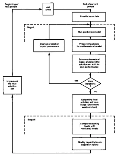
The dynamic job shop control system presented determines the best values for input and output variables for the forthcoming period based on a composite cost based performance criterion. Control is actuated on an end-of-period (EOP) basis. The general methodology is based on a two-stage analysis, as illustrated in Figure 2.

Figure 2. General Control System Methodology Performance Measures

In this paper an inputloutput control system for the dynamic job shop is presented and abbreviated DIIOCS. Its

Data for the control system comes from shop status related to jobs already in process and the status of jobs in the pool.

(3)

During the first stage analysis, an iterative search method is utilized to generate several solution sets. At each iteration, the prediction model generates forecasted data oil which the dependent variables of the mathematical model are based.

The cost performance of each iteration consists of two components: (i) cost items affected by the prediction model but not by the mathematical model (denoted as CPM), and (2) cost items affected by both the prediction model and the mathematical model (denoted as CMIP). The total cost for each iteration is denoted as CTOT where, CTOT = CPM

+

CMIP. Solution sets generated are compared by their cost performance. The minimum cost solution set is selected as the output of the first stage analysis.

The second stage analysis compares the workload levels expected to accumulate at each machine center against pre- defined norms. Capacity levels (or output variables) set by the first stage analysis are either increased, decreased, or unchanged based on these norms. Only the capacity levels are modified. The resulting solution set from this stage determines the decision variable values to be implemented in the forthcoming period.

The Mathematical Model

The mathematical model of the job shop control system establishes various relationships between shop characteristics for a planning period. These relationships are affected by input and output variables sought by the model. The objective function minimizes the sum of the expected costs of underutilization, overtime, second shift, EOP workload, WIP inventory, and tardiness, all for the forthcoming period. It includes the cost items that are directly related to the decision variable of the mathematical model. By incorporating these cost components into a single objective function, a trade-off between conflicting factors is made possible.

The primary function of the model is to determine specific values for decision variables that will give a minimum cost solution. These decision variables are of two types. The first identifies the set of jobs to be released from the pool into the shop (i.e., input control), while the other identifies the capacity levels of machines (i.e., output control). This model assumes that we are at the end of a period and that the decisions pertain to only the forthcoming period.

The following notation is used in the formulation of the problem:

i identifies jobs

j identifies machines in the shop

n = number of jobs in the pool m = number of machines in the shop

s = number of jobs in the shop at the end of the present period

f = expected number of jobs in the shop at the end of the next period

N = nominal work hours for a machine per period

CI(j) = penalty cost for one hour of idle time on machine j

CO(j) = cost of one hour of overtime on machine j

CS(j) = cost of a second shift on machine j

CL1 = penalty cost for holding one hour of workload at the end of the next period (within the first range, S K )

CL2 = penalty cost for holding one hour of workload at the end of the next period (within the second range,

>

K)

K = workload limit that defines the boundary between the first and second range

UL(j) = K minus the workload level in the first range OL(j) = workload level in the second range

CV = penalty cost for holding one hour of value in the shop

CT = cost of one hour of tardiness

SU(j) = expected idle time to be realized on machine j

in the next period

WiPs(i) = expected total value to be added on job i already in the shop

WIPp(i) = expected total value to be added on job i in the pool if it is released into the shop

TAs(i) = expected tardiness for job i in the shop

ET(X(i)) = expected tardiness for job i in the pool (dependent on whether it is released o r not)

PW(j) = present workload level of machine j at the beginning of the next period

CW(j) = workload to affect machine j during the next period from jobs already in the shop

WL(i, j ) = expected workload to affect machine j during the next period if job i is released from the pool The decision variables of the model are as follows:

X(i) = a 0, 1 variable which identifies whether job i is to be released from the pool (1 = release, 0 = do not release)

OT(j) = hours of overtime scheduled on machine j

S(j) = a 0, 1 variable which identifies whether a second shift is to be scheduled on machine j (1 = schedule,

0 = do not schedule)

The mathematical model which describes the job shop inputloutput control system is formulated as:

Min P:

2

{SU(j)*CI(j)

+

OT(j)*CO(j)

(4)

Subject to

[PW(j)

+

CW(j)

+

i

WL(i, j)*X(i)] i-l

And

Three important facton affect overall performance and the decisions in a dynamic job shop. These are: (1) the workload level, (2) the WIP inventory level, and (3) the due date status of jobs. The focus of the following sections is how these factors are incorporated into the mathematical model and a discussion of the variables which they affect.

Workload Level in the Shop

The workload level, defined as the amount of work (in hours of processing time) that is expected to affect each machine for the forthcoming period, consists of three elements: (1) the amount of work presently on each machine at the beginning of the current period [PW(j)], (2) the amount of work that will affect each machine within the next period from jobs located at other machines [CW(j)], and (3) the workload resulting from jobs being released from the pool [WL(i, j)]. The total planned machine capacity that will ac- comodate this workload consists of the nominal capacity _. _{. .}( N hours), the scheduled overtime [OT(j)], and the second shift lS(i)l.

If the total expected workload level at a given machine is less than the total scheduled capacity, then idle time [SU(j)] may be expected on machine j. In the opposite case, an expected EOP workload level [K - UL(j)

+

OL(j)] will result and is penalized at two ranges. If the level is within the first range (0 - K hours), the workload [K - UL(j)] is penalized at a rate of CL1. However, if the level is higher than K hours, the additional amount in the upper level [OL(j)] is penalized at a higher rate of CL2, where CL2 > CLl. Treating the EOP workload level in this manner forces it to attain a value within the first range.

Cost factors affected by the expected machine workload levels are as follows: cost of underutilized machine =

[SU(j)*CI(j)]; cost of overtime = [OT(j)*CO(j)]; cost of second shift = [S(j)*CS(j)]; cost of EOP workload (first range) = {[K - UL(j)laCL1); and cost of EOP workload (second range) = [OL(j)*CLZ].

The constraint that defines the relationship between the workload and the planned capacity for a specific machine j

was stated as:

[PW(j)

+

CW(j)

+

i

WL(i, j)*X(i)] i - l

The left hand side of the equation represents the total workload level plus slack (positive or negative), while the right hand side represents the total planned capacity for machine j.

WIP Inventory Level

The total value-added due to processing at the end of a period determines the WIP inventory level. Thus, WIP inventory is expressed in hours of value-added, rather than in number of jobs in the shop. There is also a significant difference between the WIP inventory level and the EOP workload level as discussed above. The former emphasizes the magnitude of the value-added to each job, while the latter represents the workload level that accumulates at each machine center at the end of a period. The EOP workload level is incorporated to force capacity increases when the limit, K, is exceeded. However, WIP inventory represents the total capital expended on the jobs. The objective in this case is to complete and ship those jobs with a high value-added status, such that the overall WIP inventory level is minimized.

WIP inventory level is represented only in the objective function. The expected total value-added to the jobs already in the shop (in total f jobs) by the end of next period is estimated from the prediction model and is denoted as WIPs(i). Since this variable is independent of the decision variables of the MIP it is included in the CPM cost component (Value = WIP,(i)*CV). The corresponding WIP inven-

i - I

tory levels due to the jobs in the pool (denoted as WIP,(i)) are multiplied by a cost factor CV ($ per hour of value- added). Only this component of the WIP is represented in the objective function because it is dependent on X(i)'s. Jobs which are expected to complete all their operations during the next period are not considered in the WIP calculations. The flow of the jobs which depend to a great extent on the waiting times realized at machines are estimated from the prediction model.

Due Date Status

An important objective in job shop control is to assure that jobs complete processing on o r before their due date. Jobs

(5)

that complete their final operation after their due date are tardy and subjected to a penalty. The difference between job completion date and its due date determines the magnitude of tardiness. For jobs already in the shop, the expected tardiness measure is denoted as TAs(i). Jobs which are early have a zero TAs(i) value. The expected completion times of the johs (which determines tardiness values) are also based on estimated waiting times. Since the tardiness values for jobs already in the shop (in totals jobs) are not dependent on the decision variables of the MIP, the cost related to this factor is included in the CPM cost component (value

1

, _ I

TAs(i) * CT)

.

Tardiness estimation is somewhat more complicated for jobs in the pool, since the decision of whether to release a job or not affects its expected tardiness measure. An expected tardiness measure (TA(i)) for all pool jobs is initially computed on the assumption that they will be released into the shop. Some jobs would have high tardiness values and others high slack values, based on their status. Jobs with high expected tardiness values are the most likely candidates for release. However, the jobs which are not released have to wait at least one period until a decision can he made regarding their release. Jobs which have an expected tardiness in this decision period will have a much higher tardiness measure by the next period if not released. The time difference between each successive period must be considered in determining the true expected tardiness measure, based on whether the job will be released or not.

The relationship that defines the expected tardiness measure under any condition is:

Z(i) is a 0 - 1 variable which attains a zero when TA(i) is positive and one when TA(i) is zero. FT(i) is the expected future tardiness at the end of the next period if job i is not released this period. In case there is an expected future slack, rather than tardiness, this value is set to zero.

A summation of the expected tardiness values for all pool jobs are then multiplied by the marginal cost of tardiness, CT ($ per hour of tardiness), to determine this cost component in the objective function. Like WIP inventory levels, estimated tardiness values are directly related to the waiting times to be realized in the shop. A prediction model is utilized to perform this estimation.

The InpuUOutput Control System (DUOCS)*

Most of the dependent variables in the mathematical model are based on estimated waiting times. Predicted waiting times are a function of the capacity levels, which are decision variables. An analytical relationship that defines the dependency between waiting times and capacity levels does not exist for the mathematical model formulated. Olhager and Rapp [9]

suggest that a non-linear relationship links waiting time and capacity utilization. However, this relationship assumes in- dependence between machines, as well as, exponential processing time distributions. Since dependencies between machines are important, this non-linear relationship was not utilized herein.

The dependent variable values of the model are determined from a prediction model analysis performed for the forthcoming period. This prediction model simulates the fonh- coming period based on fixed machine capacity settings. The outcome is a set of estimated waiting times based on these capacity levels. Running the prediction model simulation based on different capacity levels results in different waiting times. The relationship between waiting times and capacity changes is incorporated by this iterative approach, where at each iteration the prediction model capacity levels are changed. Its purpose is to evaluate different capacity level combinations and select the solution set with a minimum total cost. This generated solution set forms the basis for further analysis in the second stage.

The main events of the iterative stage analysis were illustrated in Figure 2. The mathematical model and the prediction model are embodied into the iterative procedure, which proceeds as follows: At the end of a period, initial conditions for the prediction model are determined for (1) jobs already in the shop, (2) a set of critical jobs selected from the pool (based on their due date and expected completion time), and (3) capacity levels for the machines. Thereafter, the prediction model simulates the events of the forthcoming period. Statistics and output generated from this prediction (i.e., expected waiting times at machines and the status of jobs) are utilized to compute the dependent variables of the mixed integer mathematical model (MIP). Subsequent to the prediction model analysis, the MIP is solved. The solution set and its objective function value (CMIP) is stored for further analysis. The total cost measure for this iteration consists of the objective value from the MIP (CMIP) and the costs related to factors independent of the MIP (CPM).

Costs which are independent of the MIP are: (1) cost of f WIP inventory for johs already in the shop, i.e.,

C

i = l WIPs(i)*CV, (2) cost of tardiness for the same jobs, i.e., TAs(i)*CT, and (3) cost of scheduling overtime or second 1 = 1

shifts in the prediction model (denoted as PMCOST). I

Then, CPM =

1

WIPs(i)*CV

+

2

TAs(i)*CT

+

PMCOST. i - l i- 1

These values must be included in the iteration total cost be-

'This section giver a summary description of the DllOCS. Individuals inrer- cited in more detail are encouraged to refer ro the following seelions of [ID]:

(1) Ertimatiun of the dependent variables for MIP. pp. 75-85; (2) Character- istia of the prediction model, pp. 86-91; (3) Stage I procedure of the DIIOCS, pp. 93-98; (4) Stage I1 procedure of the DIIOCS, pp. 98-102; (5) FORTRAN code for the job shop rimulatar including the DIIOCS procedure Appendix A ; (6) FORTRAN code far the FLCS simulator, Appendix 8 ; (7) MPSWMIP

code and JCL statements for executing the program on an IBM 370 MVS System, Appendix C.

(6)

cause they vary from iteration to iteration. The capacity level solution from the MIP is added to the prediction model capacity level settings to determine the final output variables for this iteration. This marks the end of an iteration.

The only variations which occur from one iteration to an- other are the prediction model capacity level settings. Each iteration results in different dependent variable values and these lead to different solutions. As an example, high capacity level settings will boost the output rate of the shop, giving low waiting times. Low waiting times will provide favorable dependent results, such as lower tardiness and WIP inventory values for the MIP. The output of the MIP, based on favorable values, will result in a solution set with a lower objective cost value. However, since these favorable dependent variable values were a result of high prediction model capacity settings, the cost of scheduling this additional capacity is also reflected in the total cost i.e., in CPM (cost of the prediction model). Thus, there are basically two opposing wst factors; high capacity level settings resulting in low MIP costs and high prediction model costs, and low capacity settings resulting in high MIP costs and low prediction model costs.

At the end of the iteration process, the minimum total wst solution is selected as the output of this stage. The number of iterations that can be performed is limited due to com- putation problems that would arise if all capacity combinations were evaluated. A six machine job shop with the option of eight, five hour overtime increments would require eval- ution of (8)6 or 262,144 different capacity combinations. Only a limited number of these are evaluated.

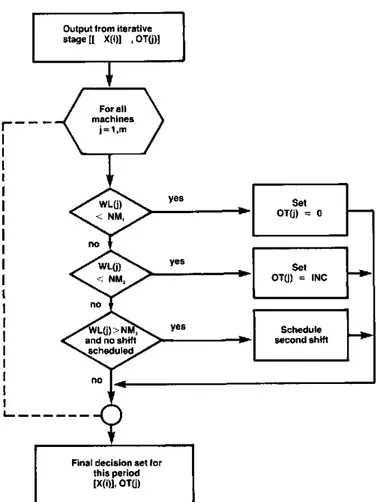
Capacity level settings from the iterative stage are subjected to re-evaluation. The purpose of this re-evaluation stage is to consider the expected workload levels that will affect each machine (estimated from the prediction model) and modify the capacity levels accordingly. Depending on these workload levels and the solution set of the iterative stage, the capacity levels are either unchanged, increased, or decreased based on norms. The steps of this stage are illustrated in Figure 3, where

INC = the increment value giving the best result in the iterative stage

NM, = norm value for the i'th workload limit (i = 1, 2 ,

3)

WL(j) = expected workload (hours of processing) to affect machine j during the next period.

An extensive simulation study was performed to determine what norms should be used to represent the limits for capacity changes. Runs were based on shop conditions with varying load levels (high, medium, low). The following criteria were used in determining the limits: (1) any reduction in capacity levels should not lead to a decrease in the machine utilization for that period, and (2) an increase in any capacity level should only be attempted when the machine is already fully utilized and when there is an expected large workload to affect this machine. The norm values determined from the sample runs were the ones that best adhered to the above criteria.

0 yec---I

s t

h

i NM, OTU) = a

OT(I) = INC

-

Final decision set lor this period

Figure 3. Procedure for Stage I I Analysis

Three norms were utilized to identify the limits for various decisions. The first two (denoted NM, and NM2) represent the workload limits for decisions about a decrease in capacity levels. The other norm (NM3) identifies the limit on whether a second shift should he considered or not. The values determined for the norms NM,, NMz, and NM3 were 20, 30, and 70 hours, respectively.

The re-evaluation procedure is as follows: If the workload level [WL(j)] is less than NM,, then the capacity level for machine j is set to only the nominal work hours (N hours). However, if WL(j) is less than NM2 and greater than NM,, then the capacity level is set to N

+

INC hours. If, on the other hand, the workload is greater than NM3 and no second shift has been scheduled as a result of the iterative stage, then a second shift is planned for that machine. After completing this procedure for all machines, the resulting modified capacity levels represent the final output decision variables for the forthcoming period.

The jobs indicated by a one in the (X(i), i = 1,

. . .

,

n)

set are released into the shop. Also overtime andior second shifts are scheduled based on the final values of the capacity levels.

The Simulation Model and Results

The DI/OCS was evaluated by comparison with an alternate control system. A hypothetical six machine job shop simulator was used in the evaluation. The job arrival process

(7)

to the shop was Poisson distributed. Four different shop load levels were simulated by choosing four different arrival rates. The total number of operations for each job was uniformly distributed between 4 and 10. The machine sequence (routing) for each job was determined from an equal probability transition matrix (i.e., a pure job shop was considered). The mean processing times for each operation was generated from a uniform distribution with parameters 3 and 9 hours. Actual operation processing times were determined when the jobs were actually on the machines and generated from a normal distribution. The processing times generated from the uniform distribution at the jobs' arrival to the shop were the mean of the distribution (p). The variance of the distribution was based on a coefficient of variation of 10%(Cv = 0.1); i.e.,

2

= ( C V * ~ ) ' . The normal distribution was truncated at

i; 3 4 to eliminate negative as well as very high values. The FCFS dispatching rule was used to determine which job to select for processing when a machine became idle.

A workload based due date assignment rule was utilized. An expected pool and shop queue time was added to the total estimated processing time to determine the expected completion time of a job. The machine queue times were based on a forecast of the average waiting times to be realized at each machine. The due date assignment rule, described in more detail in [lo], was based on the ideas of Bertrand [4].

Cost parameters of the MIP model and the EOP workload limit ( K ) were determined from a comprehensive simulation sensitivity analysis. The objective here was to set these parameters relative to each other so that a good balance among various tendencies is achieved under any shop condition. The

K, C I ( j ) , CO(j), CS(j), CL1, CL2, CV, and CTvalues were set to 15 hours, $10, $20, $700, $10, $40, $3, and $6, re- spectively.

The period was assumed to be a week, and only three iterations of the first stage analysis were performed. The main job shop simulator, coded in FORTRAN, continuously in- teracted with IBM's MPSXiMlP 370 mathematical programming package for solving the MIP's developed at each iteration. Each problem was simulated for a length of 3 years (or equivalently 150 periods).

The basic characteristics of the comparative job shop control system are: finite loading, fixed capacity, and pool oriented. We refer to this system as a Finite Loading Control System (FLCS). The main difference between the two control systems is in the degrees of control. The DIIOCS is both input and output flexible, while the comparative system is only input flexible.

Capacity levels were set at the nominal 40 hours per week for all periods. Input to the shop was controlled by a finite loading procedure. At periodic intervals, jobs were released into the shop based on the FCFS rule until the sliop was loaded to its limit. A maximum load limit of 170% of nominal capacity was set for all machines. The job arrival process, routing procedure, and the mean and actual processing times were identical to the DIIOCS simulation.

A total work content (TWK) based due date assignment rule was used for the comparative simulation runs. At the

time of a job arrival, the estimated pool waiting time was added to the total work content (sum of processing times) multiplied by a factor to determine its due date. In equation form, Due date = arrival time

+

pool time

+

factoraTWK. The factor which affects the tightness of the due dates was set to 2.6. This value resulted in approximately equal tardiness and earliness measures in sample sensitivity nms. Al- though the due date assignment rules used in hoth cases were not identical, results indicated that the rule associated with DIIOCS set tighter dates on the average than the TWK rule utilized in the comparative system. This gives the comparative system some initial advantage.

Shop load levels ranging from 70% to 90% were simulated during the runs. To accomplish this, the mean time between arrivals (MTBA) for the Poisson distrihutior. was varied four times. Each simulation trial (i.e., with one set of MTBA) was replicated ten times using different seed values. Identical random number streams were utilized in the comparative sim- ulations to provide for an unbiased painvise comparison with the DIIOCS results. Initial conditions, including the random number seed values, were identical in the same i'th replicate in hoth cases.

Statistics were collected on the following performance criteria: mean tardiness (MT), tardiness variance (VT), work- in-process inventory level per period (WIP), mean flow time (MFT), flow time variance (VFT), shop utilization (UTIL), overtime usage per period (OVER), second shift usage per period (SHIFT), and the average total cost per period ($TO- TAL). The cost parameters used are as follows: Cost of underutilization = $5.00 per idle machine hour; Cost of overtime = $12.00 per hour; Cost of extra shift = $350.00 per machine period; Cost of WIP inventory = $2.40 per hour of value added; and Cost of tardiness = $2.00 per hour of tardiness per job.

The results of the simulation runs are given in Tables 1 and 2 and illustrated graphically in Figures 4 through 7. The per- centage improvements achieved by the DIIOCS are illustrated in Table 3. A negative improvement value implies that the

FLCS performed better than the DIIOCS.

OYNAMICIID A COMPARATIVE 40

-

60

-

MT

---

VT 20

-

\ 30 \ \ 10

-

'.

15 '&--

---

--

- -

0 * 0 7.5 8.0 8.5 9.0 MEAN TIME BETWEEN ARRIVALS(HRS)

(8)

7.5 8.0 8.5 9.0

MEAN TlME B E W E E N ARRIVALS(HRS) Figure 5. MFT and VFT Performance

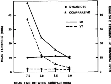
Statistical results and absolute differences in the mean values clearly indicate that the performance of the DIIOCS was superior to the FLCS, especially at highly loaded shop conditions (i.e., MTBA = 7.5). This improvement was a result of the combined input and output capability of the DI/OCS. The performance of the systems are especially important at high load levels because most problems such as backlogs, high and variable MLT, and excessive WIP inventories occur at these levels. Thus, the results at these load levels are of more interest and value than those achieved under low shop loads.

In general, at low shop loads, the differences between the

A COMPARATIVE

---

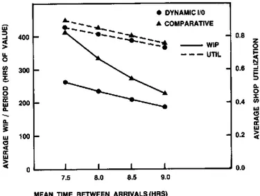
UTlL

MEAN TlME BETWEEN ARRIVALS(HRS) Figure 6. WIP lnvenioty and UTlL Performance.

performances diminished due to the absence of excessive backlogs and imbalance problems. The only measure that did not show improvement was shop utilization. This could be traced to the capacity level variations in the DIIOCS. How- ever, as observed in Figure 6, and indicated by Table 3, the magnitude of this reduction was small and insignificant as compared to the improvements achieved in other measures. The percentage reduction in the utilization measure varied from a low of 2.94 to a high of 4.77. As a trade-off for this reduction, significant improvements were achieved in MT,

VT, WIP, MFT, and VFT as summarized in Table 3.

Table 1. Performance Measures for DlIOCS shop Load (MTBA) 7.5 8.0 8.5 9.0

Table 2. Performance Measures for FLCS

March 1987, 1IE Transactions 95

Performance Measures

MT VT WIP M F T VFT UiIL OVER SHIFT $TOTAL

9.9 327.3 261.6 158.5 5507.7 0.8483 11.3 0.06 1072.81 10.4 303.4 233.2 137.5 3692.4 0.8087 9.0 0.03 1012.37 10.8 317.4 208.6 122.4 2727.0 0.7672 6.7 0.03 971.26 10.4 275.5 184.8 111.6 2109.0 0.7287 5.3 0.01 926.85 Shop Load (MTBA) 7.5 8.0 8.5 9.0

Table 3. Percentage Improvement (DIIOCS over FLCS) Performance Measures

MT VT WIP MFT VFT UTlL OVER SHIFT $TOTAL

48.2 5521.6 414.1 247.4 12565.7 0.8908 1617.39 23.9 1757.0 333.3 187.8 7364.0 0.8418 1220.56 15.4 803.0 273.6 153.3 4582.3 0.7935 1044.69 9.9 444.1 227.8 132.2 3229.7 0.7508 931.31 Shop Load (MTBA) 7.5 8.0 8.5 9.0 Performance Measures

MT VT WIP M F T VFT UTlL $TOTAL

79.41 94.07 36.82 35.93 56.17 -4.77 33.67

56.60 82.73 30.04 26.80 49.86 3 . 9 3 17.06

29.69 60.47 23.73 20.14 40.49 -3.31 7.03

(9)

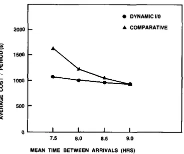
MEAN TIME BETWEEN ARRIVALS (HAS) Figure 7. Average Total Cost Performance.

2000

-

W1 1500 0 Le Y L

.

+ 1000 0 Y 500 Y

2

0

As compared to the FLCS, the two factors that had significant effects on differences were capacity flexibilities and the shop prediction function. Combined with input flexibility, significant improvements in shop control were achieved. As the WIP level dropped, this leddirectly to a reduction in flow time. Backlogs were eliminated by the use of overtime and in some cases, by the use of second shifts. But even at the highest shop load level, the overtime and second shift usages were not high (i.e., 2 hours of overtime per period).

Since no overtime was scheduled for the F'LCS, a more realistic comparison is made by observing the cost performance of the DIIOCS, which includes overtime cost. It is possible to analyze whether the improvements achieved were at the expense of high overtime and shift usage. Even with overtime cost included, the results indicated better performance by the DIIOCS as compared to the FLCS.

DYNAMIC UO

-

A COMPARATIVE

-

L

-

I I 1 I

Summary And Conclusions

7.5 8.0 8.5 9.0

A dynamic job shop control system that is both input and

output flexible was presented in this paper. Its unique characteristic is that the job release function (representing the input rate to the shop) and the capacity change function ( r e p resenting the output rate from the shop) were concurrently varied at each decision point. The job shop control problem was mathematically formulated as a 0 - 1 linear mixed integer program. The dependent variables of the MIP were determined from a prediction model that forecasts the forthcoming periods' events. Evaluation of the control system was achieved by simulating a hypothetical job shop.

The performance of the DIIOCS was compared with the performance of an alternate control system which was only input flexible. Performances were evaluated under different shop load levels with the FCFS dispatching rule. Measured performances included the total cost per period, mean flow time, flow time variance, mean tardiness, tardiness variance, WIP inventory, and shop utilization. The following conclu-

sions are drawn from the theory, simulation results, and statistical analyses:

(1) One objective was to compare the overall performance of the DIIOCS with the finite loading control system. The simulation results indicate that significant improvements in the overall performance (measured in cost) were achieved under highly loaded shop conditions. No significant improvement was observed when the shop was lightly loaded.

(2) Significant improvements were achieved for the mean flow time, flow time variance, mean tardiness, tardiness variance, and WIP inventory levels. The only inferiority observed was in the shop utilization measure, but the maximum difference was small. The cause of this inferiority could be traced to the capacity allocation function. (3) The general improvement achieved implies that the prediction model had some positive effect on performances. Although no specific analysis of the effectiveness of the prediction model was performed, it can be deduced that such a feedfonvard approach had a positive impact on the performance of the DIIOCS.

(4) The improvements achieved were attributable to the differences in the control systems rather than to differences between due date rules.

REFERENCES

[I] Ballakur, A, and Steudel, H. J., "Integration of Job ShapConlrol Sys- tems: A State-Of-me-An Review," Journal of Monufncruring Systems,

V o l 3, Na. 1, 1984. pp. 7i-79.

[2] Bechte, W., "Relationship of Order Release. WIP, and MLT." Working Paper, Southern lilinois Universiw, 1982.

[3] Belt, B., "InputIOutput Illustrated." Production and inventory Man- agemen,, 2nd Quaner, 1978.

[4] Benrand, J . W. M., "The Effect of Workload Dependent Due-Dates

on Job Shop Peltormanee," Monogernenr Science. Vol. 29, No. 7, 1983,

pp. 799-816.

[5] Bcnrand. J. W. M. and Wonmann, I. C., Producrion Control and ln- formanion Sysrem for Component-Monufoeturing Shops. Elaevier ki-

entific Publishing Ca., Amsterdam, 1981.

[6] Fabrycky. W. I . , "Pmbsbilirtic Procedures for Sequencing and for Con- trolling Machine Center Capacltier in Jab Shops." Proceedings, Second Annual Systems Engineering Conference of lke AIIE, November, 1974.

[7] Irastorza, J . C. and Deane, R. H . . "A Laading and Balancing Method

far Job Shop Control," AIIE Tromocrions, Vol. 6, No. 4. 1974, pp. 302- 307.

181 Karni, R., "Capacity Requirements Planning-A Systemization." infer- notional Jourool of Producrion Research, V o l 20, No. 6, 1982. pp. 715- 739.

[9] Olhager. J. and Rapp. B., "Balancing Capacity and Lot Sizes," European Jourml of OperarionalJolournal, Vol 19, 1985, pp. 337-344.

1101 Onur. L.. 'A Dynamic InputtOutput Control System forlobShopMan- ufacturing Operations," Unpublished Ph.D. Dirrcnation, Virginia Polyrechnic InrIiture ond Store Univeniry, 1985. Available through Uni-

versity Microfilms.

[ I l l Shimoyaihira, S., Iroda. K. and Awane, H., "laput SehedulingandLoad Balance Control for A Job Shop," lnrernotionol lournnl of Produclion

Research, V o l 22, No. 4. 1984, pp. 5 9 - 6 3 s .

112) Tatsiopoulor. I. P, and Kingsman, B. G., ''Lead Time Management,"

(10)

Wolter J. Fabrycky is Proferror af lndustrial Engineering and Operations Research at Virginia Polytechnic lnstitutc and State Univenity. He received the Ph.D. in Engineering in 1962 from Oklahoma State University, the M.S.

in Industrial Engineeting in 1958 from the University of Arkansas, and the B.S. in Industrial Engineering in 1957 from Wichita State University. Dr. Fab~ycky taught at Arkansas and Oklahoma State and then joined Virginia Tech in 1965 where he rerved as Associate Dean of Engineering and then ar

Dean of Research. H e was elected to the rank of Fellow in the American lnrtituteof Industrial Engineers in 1978and the rankof Fellow in the American Association for the Advancement of Science in 1980.

Dr. Fabrycky is w-author of five Prentiee-Hall b o k s . There are: Procure- ment and Invenrory Sy~tems Analysir (1981). Applied Operatiom Research and

Monngement Science (1984), Engineering Economy (1984), Sysrems Engineer-

ing and Amlysir (198th and Economic Decision Analysis (1980). He also co-

edits the Prcntiee-Hall International Series in lndustrial and Systems Engi-

neering.

Levent Onur is an assistant professor in the Depanment of Indurtrial En- gineering at Bilkent University, Turkey. He graduated from Aston Univenity with a B.Se. degree in Production Engineering in July. 1978. Dr. Onur worked for the Lucai Company in Birmingham, England for a period of 9 months.

He entered Stanford University in September 1979 and earned a Master oi k i e n c e degree in Industrial Engineering. He thereafter returned t o Turkey and worked in industry. After a year of work, he entered Virginia Tech in September 1981 as a candidate far the P h . D degree in Industrial Engineering and Operations Research. He w r k e d for Philip Morris Ine. and VSE Cor-

poration during the summers' of 1982 and 1984, respectively. After completing his P h . D degree in August 1985, Dr. Onur joined the faculty o f t h e Industrial Engineering Depanment at Cleveland State University for one year.

He is a member of IIE, SME, and rhe industrial engineering honor society Alpha Pi Mu.