A
Connectionist Approach
Kemal OflazerDepartment of Computer Engineering and lnformation Science, Bilkent University, Bilkent, Ankara, 06533 Turkey*
We present a connectionist approach for solving Tangram puzzles. Tangram is an ancient Chinese puzzle where the object is to decompose a given figure into seven basic geometric figures. One connectionist approach models Tangram pieces and their possible place- ments and orientations as connectionist neuron units which receive excitatory connec- tions from input units defining the puzzle and lateral inhibitory connections from compet- ing or conflicting units. The network of these connectionist units, operating as a
Boltzmann Machine, relaxes into a configuration in which units defining the solution receive no inhibitory input from other units. We present results from an implementation
of our model using the Rochester Connectionist Simulator. 0 1993 John Wiley & Sons, Inc.
I. INTRODUCTION
Tangram is an ancient Chinese puzzle in which the objective is to decom- pose a given figure into seven basic geometric figures.' (Henceforth, we will refer to these geometric figures as Tangram pieces, or pieces for short.) Tangram figures may belong to a broad spectrum, varying from geometrical Tangrams, such as triangles, trapezoids, or parallelograms, to representational ones, such as human figures. Our previous work has used traditional artificial intelligence and computational geometry techniques to solve these puzzles.* In this article, we present a connectionist approach for solving Tangram puzzles. Our connec- tionist approach models Tangram pieces and their possible placements and orientations as units which receive excitatory connections from input units defining the puzzle and lateral inhibitory connections from competing units. The system of units operating as a Boltzmann Machine relaxes into a configuration in which units defining the solution receive no inhibitory input from others. We have implemented this connectionist model using the Rochester Connectionist Sirnulato9 and present results from our implementation.
*E-mail: [email protected]; fax: (90)-4-266-4127.
INTERNATIONAL JOURNAL OF INTELLIGENT SYSTEMS, VOL. 8,603-616 (1993) 0 1993 John Wiley & Sons, Inc. CCC 0884-8173/93/050603-14
Figure 1. The Tangram pieces: 1,2--large triangles; 3-square; 4-medium triangle: 5-parallelogram; 6,7-small triangles.
The seven-piece set of Tangram is cut from a square as shown in Figure 1. The small triangles are called basic triungles. The other pieces are all composi- tions of basic triangles. The rules of Tangram are self-evident: the given figure is to be decomposed into the Tangram pieces, and the decomposition has to use all seven pieces. For example, in Figure 2, part (a) shows a Tangram that depicts a running man, and part (b) gives the solution for that Tangram.
11. GRID TANGRAMS
Grid Tangrams constitute a subclass of Tangrams in which every vertex of each
of
the seven pieces that comprise the Tangram coincides with the pointson a square grid. The grid points are separated from each other by unit length,
Figure 2. solution.
the edge length of the square piece (cf. Fig. 1). (Figure 12 later in the article gives some examples of grid Tangrams and their solutions.)
111. CONNECTIONIST MODELS
Connectionism has come out as novel paradigm in artificial intelligence owing to results of the work of the past decade. The basic computational paradigm is based on a network of a massive number of simple processing units whose functionality models that of real neuron^.^,^ There have been a tremendous number of applications of this computational paradigm in widely varying areas, such as cognitive science, signal processing, combinatorial opti- mization, and so forth. In the latter, such network models have been used to obtain approximate solutions to a number of well known hard
problem^.^,'
Connectionist models have been applied to solving puzzles by Kawamoto,8 who has used an autoassociative network with some extensions to implement hill- climbing for solving a number of puzzles, including the DOG j CAT puzzle, where the objective is to generate a sequence of three-letter words starting with
DOG and ending with CAT, changing one letter at a time. Takefuji' has used a
neural network model to obtain a parallel algorithm for tiling a grid with polyo- minoes.
A. Boltzmann Machines
Our approach in this work uses a Boltzmann Machine modello for solving grid Tangram puzzles. Boltzmann Machines are neural network models that are specifically applicable to constraint satisfaction problems which can be (approximately) solved by relaxation search. They combine the Hopfield model" with the simulated annealing paradigm12 to perform relaxation search through a state space. Contrary to Hopfield networks, where the state space search may get stuck in local minima of the energy measure being minimized, Boltzmann Machines introduce a probabilistic component to the state change decision of the neuron units along with the concept of a Temperature parameter to simulate annealing. The basic idea behind Boltzmann Machine operation is the following: Each neuron unit computes a weighted sum of the inputs that are connected to it. If the sum exceeds the unit's threshold then the output of the unit is set to 1, indicating active unit state. If, however, the sum is below the threshold, the output is determined by a probability distribution (described in Sec. IV-D). The unit's output may be set to 1 with a certain probability deter- mined by the distribution. Thus, instead of only moving downhill towards a minimum, the network exhibits some random behavior so that it may occasion- ally go uphill in the energy space to skip over or jump out of local minimum and not get stuck there.
The probability distribution that determines this random behavior is a function of a parameter commonly called the Temperature in reference to the use of temperature in the process of annealing.'* The higher the temperature, the higher the probability a unit may turn on even though its net input is below
I I I
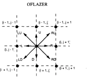
Figure 3. Representation of grid points by a group of eight units.
the threshold. During the network's operation, the temperature is reduced slowly, reducing the chances that a unit may switch on with a given net input. Boltzmann Machines are especially suited for constraint satisfaction prob- lems where neuron units represent hypotheses and the connections between units represent constraints among hypotheses. Hypotheses that mutually rein- force each other have positive weights on their mutual connections, while competing hypotheses have negative weights. However, such machines are more suited to deal with weak constraints, where the problem is to find a configuration of units in which the most important constraints (indicated by connection strength) are satisfied. This is in contrast to hard constraint prob- lems, where the objective is to find a configuration where all constraints are satisfied. Solving Tangram puzzles involves satisfying a number of hard con- straints, but as will be seen below, Boltzmann Machines have been successful
in solving this problem.
IV. A CONNECTIONIST MODEL FOR GRID TANGRAMS
A. Representing the Puzzle
Our model represents a grid Tangram puzzle as sets of active units repre- senting grid points covered by the puzzle. Since such Tangrams may have holes
or
concave boundaries, we have chosen to represent each grid point by a set of eight units as shown in Figure 3. The grid points are labeled with coordinates(i,
j ) , i indicating the row and j indicating the column in the grid in standard matrix notation. The eight units associated with each grid point indicate in which orientations the puzzle area or boundary extends around that grid point. The orientations are: Left (L), Right (R), Down (D), Up(U),
Right-Up (RU), Right-Down (RD), Left-Up(LU),
and Left-Down (LD).A
grid Tangram puzzle is represented by externally setting the grid units for relevant orientations of each point covered by the puzzle. For example, a grid point that is totallyU
LYRu
D D
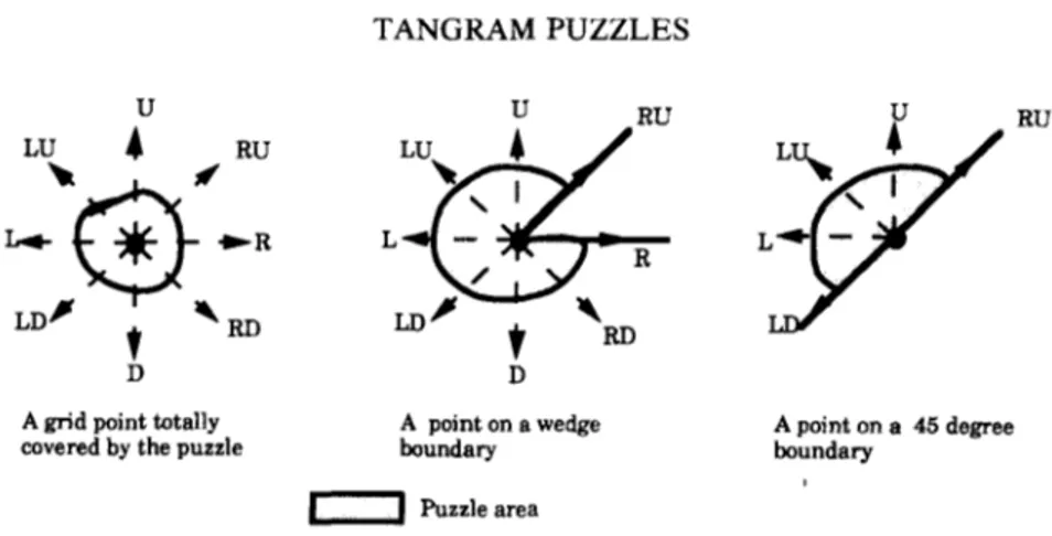
A grid point totally
covered by the puzzle boundary boundary
A point on a wedge A point on a 45 degree
C‘
Puzzle areaFigure 4. Representation of the puzzle space around a grid point by orientation units. covered by the puzzle has all of its orientation units on;
so
does a point that is on a boundary but has a wedge missing, as shown in Figure4.
Figure 5 shows a complete example of the representation of a grid Tangramin
our model. The reader may notice that there is a rather superficial similarity between our representation and Freeman’s “chain code.”13B. Representing the Tangram Pieces
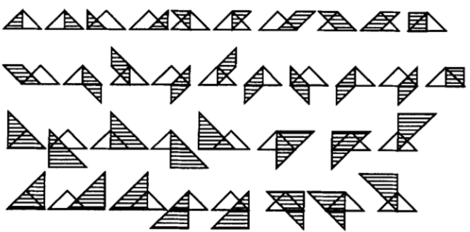
In grid Tangrams, the placement and orientations of the base puzzle pieces are limited. For example, the only way that the square piece can appear is when its corners are on the grid. There are four possible orientations of each of the other pieces: 0 1 2 3 (0,O): R, RD, D (0,l): L, LD, D, RD, R (0,2): L, LD, D, RD (1,O): U, RU, R, RD,D (1.1): L, L U , U, RU, R, RD, D, LD (1,2): L, LU, U, RU, R, RD, D (1,3): LU, L, LD, D (2,O): U, RU, R, RD, D ( 2 , l ) : L, LU, U, RU, R, RD, D, LD (2,2): L, LU, U, RU, R, RD, D, LD (2,3): U, LU, L, LD, D (3,O): U, RU, R (3,l): L, LU, U, RU, R (3,2): L, L U , U , RU, R (3,3): U, LU, R
Figure 5. An example puzzle representation showing the orientation units activated for grid points covered by the puzzle.
small triangle medium triangle square
large triangle parallelogram
Figure 6. Orientations and labeling of Tangram pieces.
(1) Small triangles can appear in orientations Left-Up (LU), Left-Down (LD), Right-Up (RU), and Right-Down (RD), depending on where the right-angle corner of the triangle is placed with respect to the grid point ( i , j ) . If the corner is on point ( i , j ) then it is in LU orientation, if the corner is on point ( i
+
1, j ) then it is in LD orientation, if the corner is on ( i , j+
1) then it i? in RU orientation, and when the corner is on ( i+
1 , j+
1) it is in RD orientation. When we talk about the “LD small triangle at ( i , j ) , ” we mean the triangle with the right-angle corner at ( i+
I , j ) with the other corners placed at ( i , j ) and ( i+
1, j+
1).( 2 ) Medium triangle can appear in orientations Up (U), Down (D), Left (L), and Right (R), depending on where the right-angle corner points to. For example, when we talk about the “R medium triangle at ( i , j),” we mean the medium triangle with the right-angle corner at ( i
+
I , j+
1) and the two other corners at ( i , j ) and ( i+
2 , j ) . Similarly, a U medium triangle at ( i , j ) has its right-angle corner on ( i , j+
1) and its two other corners at ( i+
1, j ) and ( i+
1, j+
2 ) .(3) Parallelogram can appear in orientations L, R, U, and D. In the U and D orientations the longer dimension is along the vertical axis, and in L and R orientations the longer dimension is along the horizontal axis. For example, the “ L parallelogram at (i, j)” has its corners at (i, j ) , ( i , j
+
l), ( i+
1, j+
l), and ( i+
I , j+
2 ) .(4) Large triangle can be placed in the same orientations as the small triangle-that is, LU, LD; RU, RD--except that these pieces are larger. For example, the
“RD Large triangle at ( i , j ) ” has its right-angle corner at ( i
+
2 , j+
2 ) , and the two other corners at ( i , j+
2 ) and ( i+
2, j ) .Because the grid is finite, certain placements of the pieces around the boundary are not applicable. Figure 6 shows the set of possible orientations for all th e pieces.
In a grid of size I rows by J columns, there are 4(1 - 1)(J - 1) possible
placements of a small triangle, ( I - l)(J - 1) placements of the square,
2(1 - I)( J - 2)
+
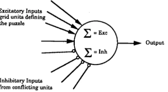
2(1 - 2)(5 - 1) possible placements for the medium triangleand the parallelogram, and 4(1 - 2)(5 - 2) placements for a large triangle. I n our connectionist model, all these placements of pieces are represented by neuron units (depicted in Figure 7) which receive excitations from input units representing the grid area covered by the puzzle a nd inhibitory inputs from the outputs of other conflicting neuron units. They sum their inputs and determine
Excitatory Inputs grid units defining the puzzle
o u t p u t = Inh
Inhibitory Inputs from conflicting units
Figure 7. A neuron unit representing a single placement and orientation of a Tangram piece.
their output probabilistically in the manner described in Sec. 1V.D. For example,
the unit representing a square at
(i,
j ) receives excitatory inputs from the following grid orientation units:(1) For grid point (i, j ) : R, RD, and D units.
( 2 ) For grid point (i, j
+
1): L, LD, and D units. (3) For grid point (i+
I , j ) : U , RU, and R units. (4) For grid point (i+
1, j+
1): U, LU, and L units.Similarly for instance, the unit representing a LD large triangle receives excit- atory inputs from the following grid orientation units:
(1) For grid point (i, j ) : D, RD units.
( 2 ) For grid point ( i
+
1, j ) : U , RU, R, RD, D units. (3) For grid point ( i+
2, j ) : U, RU, R units.(4) For grid point ( i
+
1, j+
1): LU, L, LD, D, RD units.(5) For grid point ( i
+
2 , j+
1): L, LU, U, RU, R units. (6) For grid point ( i+
2 , j+
2): LU, L units.Figure 8 shows the inputs for one orientation of each of the five distinct
Tangram pieces.
C. Representing Placement Constraints
Any unit that has at1 of its excitatory inputs active can be part of a solution of the given grid Tangram puzzle provided it does not conflict with another unit. The conflicts can be in one of two ways:
(1) Only one of the units representing a class of units (e.g., squares) can be active (2) A given piece of area on the puzzle can be covered by only one piece, hence
as there is only one such piece in the puzzle set.* only one of the units covering an area can be active.
*For convenience, we treat the second small and large triangles as distinct classes of units, which just happen to have the same shape as their counterpart.
LU-small triangle U-medim- triangle
(i, j+O (i, j+2)
(i+l, j+2) (i+l, j+l)
(i+2, j+2)
D-parallelogram RD-large triangle
Arrows originating from L grid point indicate the grid point orientation units sending exdta- tory input to the units repreoenting the piece with the given orientation.
Figure 8. Excitatory inputs to some of the units.
These constraints are represented by lateral inhibitory links between con- flicting units. For the first set of the constraints above, we use a standard winner- take-all network organizati~n.~ All units within a single class (e.g., squares or medium triangles) are linked to each other with inhibitory links representing the fact that only one of them can be active. Thus, within the resulting connectionist network for a given Tangram puzzle, there are seven separate such winner- take-all networks.
For the second set of constraints, we establish mutually inhibitory links between any two units representing piece orientations and placements whose areas of coverage intersect. For example, Figure 9 shows all the other kinds and orientations of pieces corresponding to the units with which a single UP medium triangle unit has mutually inhibitory links. These correspond to the second set of constraints above. The inhibitory links enforcing the first set of constraints handles overlaps with other medium triangles. Thus, in the solution, a given piece of area of the puzzle is covered by only one piece which inhibits all other competing pieces.
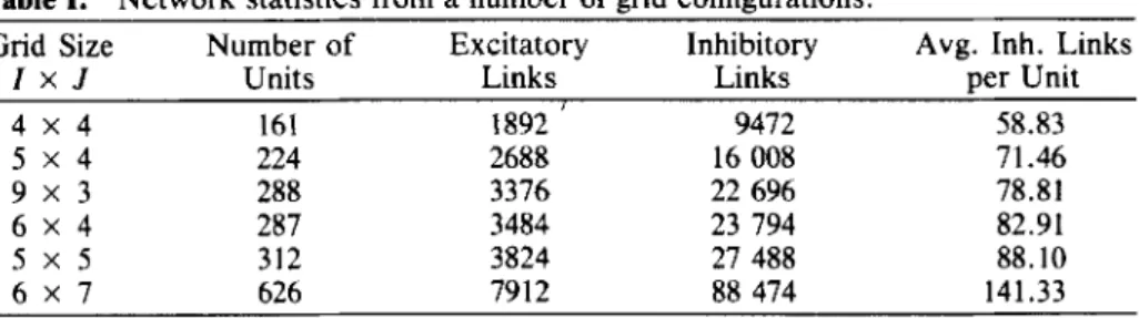
Figure 10 shows the general architecture of the resulting network and Table I shows some network statistics from a number of different grid configurations.
Figure 9. Piece orientations for units (shaded) mutually inhibitory with unit for a medium triangle piece in the UP orientation (white).
Units for Square
the puzzle area
Inhibitory Connections
among unita for a given piece
enforcing the fact that there 8hOkd be o d y on occurrenee of the piece in the eolution for preventing pieces fmm
covering overlapping area mangle 2
of the puzzle
Table I. Network statistics from a number of grid configurations.
Grid Size Number of Excitatory Inhibitory Avg. Inh. Links
I x J Units Links Links per Unit
4 x 4 161 1892 ' 9472 58.83 5 x 4 224 2688 16 008 71.46 9 x 3 288 3376 22 696 78.81 6 x 4 287 3484 23 794 82.91 5 x 5 312 3824 27 488 88.10 6 x 7 626 7912 88 474 141.33
It should be noted that the average number of inhibitory links per unit is rather high.
We use the following approach for setting the weights:
For
the excitatory links from the grid input units the link weights are set to 1/G, where G is the number of grid point orientation units that are connected to a given unit.* Forthe inhibitory links we use a link weight
-
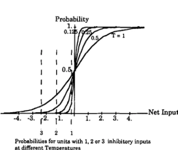
1.1, so that a unit with all excitatory inputs 1 and one inhibitory input active gets a net input of - 0.1, which gives it a reasonable probability of switching on. Figure 11 shows a plot of the logistic function and the probability of a unit's changing state for different temperatures and number of inhibitory inputs.This network operates as a Boltzmann Machine where units determine their output according t o a certain probability distribution which changes de- pending on a Temperature parameter T, which is slowly reduced as time pro- gresses.
D. Operation of the Network
Once the network is constructed, the grid units corresponding to the grid points covered by the puzzle are activated and these send excitatory inputs to all the units. With T set to its initial value, the units start operating in the following manner:
If the total excitatory input to the unit is less than 1.0 (i.e., some of the underlying grid units are not active), then the output of that unit is set to 0 since this unit can never be a part of the solution.
If the total excitatory input to the unit is 1 .O and there is no inhibitory input, the unit output is set to 1.0.
0 If the total excitatory input to the unit is 1.0, the unit output is set to 1.0 with a
probability p = l/(l f e where net = 1
+
inh is the net input to the unit with inh being the total inhibition (hence negative). Thus units receiving a slightly negative net input (i.e., only one inhibitory input active) have a good chance (around 0.5 when the temperature is high) to turn on, while units receiving more inhibitory input have a much poorer chance of turning on.*The only reason the weights are selected in this way is that when all the excitatory inputs to a unit are active then the net excitatory input to a unit will be 1. C = 7 for the small triangle units, 12 for square, medium triangle and parallelogram units, and 22 for the large triangle units.
Probability
Net Input
3 2 1
Probabilities for units with 1.2 or 3 inhibitory inputs at different Temperatures
Figure 11. The logistic probability function for Boltzmann Machines
In a cycle, the network of units are updated in an asynchronous manner in a random order determined by the simulator. T is reduced by a factor of 0.9 after every Z iterations determined by the cooling schedule. Thus as the temperature “cools down,” the probability of a unit with a given negative net input switching on is reduced. If, in three consecutive cycles, no units change state, then this is interpreted to be a local extremum and the temperature is slightly raised to force the network out. For all puzzles with which we have experimented, the corresponding networks have converged to a solution in which seven active units do not receive any inhibitory inputs.
E. Results
We have modeled a number of grid Tangram puzzles using the model described above. Ten such puzzles are shown in Figure 12. We have tried a number of cooling schedules for the Boltzmann Machine by changing the initial temperature and the temperature change cycle-obviously many similar sched- ules are possible. Table 2 shows the number of cycles required for converging to a solution for the puzzles shown in Figure 12 for four cooling schedules. It
can be observed that no schedule is in general better than the others. It is also
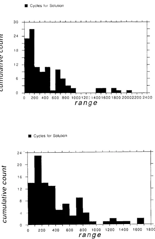
possible to change the strength of the inhibitory connections to more negative values and get a (possibly) slightly different behavior. Figure 13 shows the plot of the range of cycles required for convergence to a solution vs the cumulative count of the runs, for 100 runs of two puzzles (puzzles 7 and 10) using the last schedule in Table 11. The only difference among these runs is the initial random number seed that determines the order of updates. It can be seen that a large percentage ( ~ 7 0 % ) of runs converge to a solution in relatively small number of iterations ( 4 0 0 ) in both cases.Puzzle 1 Puzzle 2 Puzzle 5 Puzzle 3 Puzzle 6 Puzzle 4 Puzzle 7 Puzzle 8 Puzzle 9 Puzzle 10 Figure 12. Some grid Tangram puzzles and their solutions.
V. CONCLUSIONS
We have presented a connectionist model for solving grid Tangrams based
on the Boltzmann Machine model. This model represents the placements and orientation of the Tangram pieces by units which receive excitatory inputs from grid point units included in the puzzle area. The placement constraints between the units are represented by inhibitory links between conflicting units. W e
have implemented this model using the Rochester Connectionist Simulator and presented results from our implementation. Our results show that the networks constructed for a variety of puzzles converge in a few hundred iterations.
Table 11. Cycles required for solution for various Boltzmann Machine cooling sched-
ules. To is the initial temperature and I is the number of cycles after which the temperature
is reduced bv 0.9. ~~ -~ Sch. Puzzles Tn I 1 2 3 4 5 6 7 8 9 10 1.0 10 618 392 934 129 1603 201 605 249 350 197 1.0 5 1423 188 103 92 2254 108 200 548 705 534 0.5 10 101 80 1459 377 255 353 225 276 332 201 1.0 5 1055 763 783 2079 791 756 184 1291 464 70
.(r
c
3 0 0E
3 0 2 4 1 8 1 2 6 0 0 2 0 0 4 0 0 6 0 0 8 0 0 1 0 0 0 1 2 0 5 1 4 0 0 1 6 0 0 1 8 0 0 20002200 2 4 0 0r a n g e
W Cycles for Solulion
I I I I I 1 1 I I
0 2 0 0 4 0 0 600 8 0 0 1 0 0 0 1 2 0 0 1 4 0 0 1 6 0 0 1 8 0 0
r a n g e
References
1. J . Elffers, TANGRAM, The Ancient Chinese Shapes Game (Penguin, London, 1976). 2. Z. Gungordu and K. Oflazer, “Solving Tangram puzzles,” in Proceedings of ISCIS
VK-International Symposium on Computer and Information Sciences, M. Baray
and B. Ozgiiq, Eds., Elsevier, Amsterdam, 1991, Vol. 2, pp. 691-702.
3 . J.A. Feldman, M.A. Fanty, and N.H. Goddard, “Computing with structured neural networks,” Commun. ACM 31(2), 170-187 (1988).
4. J. McClelland, D. Rumelhart, and the PDP Research Group, Parallel Distributed
Processing: Explorations in the Microstructure of Cognition, Vol. 2 (MIT, Cam-
bridge, MA, 1986).
5 . J.A. Feldman and D.H. Ballard, “Connectionist models and theirproperties,” Cogn.
Sci. 6, 205-254 (1 982).
6. J . Hopfield and D. Tank, “ ‘Neural’ computation of decisions in optimization prob-
lems,” B i d . Cybern. 52, 141-IS2 (1985).
7. A. Kahng, “Travelling salesman heuristics and embedding dimension in the Hopfield model,” in International Joint Conference on Neural Networks, (IEEE, New York,
8. A.H. Kawamoto, “Solving puzzles with a connectionist network using a hill-climb- ing heuristic,” In Proc. of the Conference on Cognitive Science, (Lawrence Erlbaum
Associates, Hillsdale, 19861, pp. 514-521.
9. Y. Takefuji and K.-C. Lee, “A parallel algorithm for tiling problems,” IEEE Trans.
Neural Networks, 1(1), 143-145 (1990).
10. D. Ackley, G. Hinton, and T. Sejnowski, “A learning algorithm for Boltzmann machines,” Cogn. Sci. 9, (1985).
1 1 . J. Hopfield and D. Tank, “Computing with neural circuits: A model,” Science 233, 12. S. Kirkpatrick, C.D. Gelatt, and M.P. Vecchi, “Optimization by simulated anneal- 13. H. Freeman, “Computer processing of line-drawing images,” ACM Comput. Suru.
1989), Vol. 1, pp. 513-520.
625-633 (1986).
ing,” Science 220(4598), 671-680, (1983). 6(1), 57-93 (1974).