Search for production of Higgs boson pairs in the four b quark final state using large-area jets in proton-proton collisions at root s 13 TeV

CERN-EP-2018-195 2019/01/23

CMS-B2G-17-019

Search for production of Higgs boson pairs in the four b

quark final state using large-area jets in proton-proton

collisions at

√

s

=

13 TeV

The CMS Collaboration

Abstract

A search is presented for pair production of the standard model Higgs boson using data from proton-proton collisions at a centre-of-mass energy of 13 TeV, collected by the CMS experiment at the CERN LHC in 2016, and corresponding to an integrated

luminosity of 35.9 fb−1. The final state consists of two b quark-antiquark pairs. The

search is conducted in the region of phase space where one pair is highly Lorentz-boosted and is reconstructed as a single large-area jet, and the other pair is resolved and is reconstructed using two b-tagged jets. The results are obtained by combining this analysis with another from CMS looking for events with two large jets. Lim-its are set on the product of the cross sections and branching fractions for narrow bulk gravitons and radions in warped extra-dimensional models having a mass in the range 750–3000 GeV. The resulting observed and expected upper limits on the non-resonant Higgs boson pair production cross section correspond to 179 and 114 times the standard model value, respectively, at 95% confidence level. The existence of anomalous Higgs boson couplings is also investigated and limits are set on the non-resonant Higgs boson pair production cross sections for representative coupling values.

Published in the Journal of High Energy Physics as doi:10.1007/JHEP01(2019)040.

c

2019 CERN for the benefit of the CMS Collaboration. CC-BY-4.0 license

∗_{See Appendix A for the list of collaboration members}

1

Introduction

In the standard model (SM), Higgs boson (H) [1–3] pair-production can occur through several subprocesses and is sensitive to the Higgs boson self-coupling. In proton-proton (pp) collisions at the CERN LHC, the SM HH production cross section is mainly due to the gluon-gluon fusion subprocess, which proceeds via an internal fermion loop dominated by the top quark, t. At a

centre-of-mass energy of 13 TeV, this cross section is 33.5+₋2.5_2.8fb [4–6], which is too small to be

observable using the current data. However, many beyond the standard model (BSM) theories predict higher rates of Higgs boson pair production. The rate could be increased through the production of a massive BSM resonance X, which subsequently decays to a Higgs boson pair

(X → HH) [7], a process that could be observable at the LHC. If the resonance mass mX is too

large for X to be directly produced in pp interactions, the particle could manifest itself through off-shell effects, leading to anomalous couplings of the H boson to the SM particles, including the HH self-interaction [8]. Thus, BSM effects may modify the HH differential and integral production cross sections, making this process observable with current data.

Models with a warped extra dimension (WED), as proposed by Randall and Sundrum [7], are among those BSM scenarios that predict the existence of resonances with large couplings to the SM Higgs boson, such as the spin-0 radion [9–11] and the spin-2 first Kaluza–Klein (KK) excitation of the graviton [12–14]. The WED models postulate an additional spatial dimension l compactified between two four-dimensional hypersurfaces known as the branes, with the region between, the bulk, warped by an exponential metric κl, where κ is the warp factor [15].

A value of κl∼35 fixes the mass hierarchy between the Planck scale MPland the electroweak

scale [7]. One of the parameters of the model is κ/MPl, where MPl≡ MPl/

√

8π. The ultraviolet

cutoff scale of the modelΛR ≡

√

6e−κl_M

Pl[9] is another parameter, and is expected to be near

the TeV scale.

In the absence of new resonances coupling to the Higgs boson, the gluon fusion Higgs boson pair production subprocess can still be enhanced by BSM contributions to the coupling pa-rameters of the Higgs boson and the SM fields [16]. The SM production rate of HH through

gluon fusion is determined by the Yukawa coupling of the Higgs boson to the top quark ySM_t

and the Higgs boson self-coupling λSM_HH = m2_H/2v2. Here, mH = 125 GeV is the Higgs boson

mass [17, 18] and v = 246 GeV is the vacuum expectation value of the Higgs field. Deviations

from the SM values of these two coupling parameters can be expressed as κλ ≡ λHH/λSM_HH

and κt ≡yt/ySMt , respectively. Depending on the BSM scenario, other couplings not present in

the SM may also exist and can be described by dimension-6 operators in the framework of an effective field theory by the Lagrangian [19]:

L_H=1 2∂µH∂ µ_H−1 2m 2 HH2−κλλSMHHv H3− mt v (v+κtH+ c2 v HH) (tLtR+h.c.) + 1 4 αs 3πv(cgH− c2g 2v HH)G µν_G µν.

The anomalous couplings and the corresponding parameters in this Lagrangian are: the contact

interaction between a pair of Higgs bosons and a pair of top quarks (c2), the interaction between

the Higgs boson and the gluon (cg), and the interaction between a pair of Higgs bosons and a

pair of gluons (c2g). The couplings with CP-violation and the interactions of the Higgs boson

with light SM and BSM particles are not considered. The Lagrangian models the effects of BSM scenarios with a scale that is beyond the direct LHC reach. This five-parameter space of BSM Higgs couplings has constraints from measurements of single Higgs boson production and other theoretical considerations [20, 21].

Collaborations using the LHC pp collision data at√s = 8 and 13 TeV. A search targeting the

high mXrange for a KK bulk graviton or a radion decaying to HH, in the bbbb final state, was

published by the CMS Collaboration [39], in which two large-area jets are used to reconstruct the highly Lorentz-boosted Higgs bosons (“fully-merged” event topology). A similar search,

focusing on a lower range of mX, was also performed by CMS [40], using events with four

separate b quark jets. The configuration of a Higgs boson candidate as one large-area jet or as two separate smaller jets is dependent on the momentum of the Higgs boson [41].

In this paper, we improve upon the CMS search for high mass resonance (750≤mX≤3000 GeV)

decaying to HH→bbbb [39] by using “semi-resolved” events, i.e. those containing exactly one

highly Lorentz-boosted Higgs boson while the other Higgs boson is required to have a lower

boost. The data set corresponds to an integrated luminosity of 35.9 fb−1 from pp collisions at

13 TeV. The more boosted Higgs boson is reconstructed using a large-area jet and the other is reconstructed from two separate b quark jets. The inclusion of the semi-resolved events leads to

a significant improvement in the search sensitivity for resonances with 750≤ mX ≤ 2000 GeV.

With the addition of the semi-resolved events, a signal from the non-resonant production of HH is also accessible using boosted topologies, since such production typically results in an HH invariant mass that is lower than that of a postulated resonance signal. For full sensitivity, the results are obtained using a statistical combination of the semi-resolved events with the fully-merged events selected using the criteria in Ref. [39]. In addition to improving the search

for X→HH, strong constraints are thus obtained for several regions in the H boson anomalous

coupling parameter space, defined by Eq. (1).

2

The CMS detector and event reconstruction

The CMS detector with its coordinate system and the relevant kinematic variables is described in Ref. [42]. The central feature of the CMS apparatus is a superconducting solenoid of 6 m internal diameter, providing a magnetic field of 3.8 T. Within the field volume are silicon pixel and strip trackers, a lead tungstate crystal electromagnetic calorimeter (ECAL), and a brass and scintillator hadron calorimeter (HCAL), each composed of a barrel and two endcap sections.

The tracker covers a pseudorapidity η range from −2.5 to 2.5 with the ECAL and the HCAL

extending up to |η| = 3. Forward calorimeters in the region up to |η| = 5 provide good

hermeticity to the detector. Muons are detected in gas-ionization chambers embedded in the

steel flux-return yoke outside the solenoid, covering a region of|η| <2.4.

Events of interest are selected using a two-tiered trigger system [43]. The first level (L1), com-posed of custom hardware processors, uses information from the calorimeters and muon de-tectors to select events at a rate of around 100 kHz. The second level, known as the high-level trigger (HLT), consists of a farm of processors running a version of the full event reconstruc-tion software optimized for fast processing, and reduces the event rate to around 1 kHz before data storage. Events used in this analysis are selected at the trigger level based on the presence of jets in the detector. The level-1 trigger algorithms reconstruct jets from energy deposits in the calorimeters. The particle-flow (PF) algorithm [44], aims to reconstruct and identify each individual particle in an event. The physics objects reconstructed include jets (clustered with a

different algorithm), electrons, muons, photons, and also the missing-pTvector.

Multiple pp collisions may occur in the same or adjacent LHC bunch crossings (pileup) and contribute to the overall event activity in the detector. The reconstructed vertex with the largest

value of summed physics-object p2_Tis taken to be the primary pp interaction vertex. The physics

tot he vertex as inputs, and the associated missing transverse momentum, taken as the

nega-tive vector sum of the pT of those jets. The other interaction vertices are designated as pileup

vertices.

The energy of each electron is determined from a combination of the electron momentum at the primary interaction vertex as determined by the tracker, the energy of the corresponding ECAL cluster, and the energy sum of all bremsstrahlung photons spatially compatible with originating from the electron track. The energy of each muon is obtained from the curvature of the corresponding track. The energy of each charged hadron is determined from a combi-nation of its momentum measured in the tracker and the matching ECAL and HCAL energy deposits, corrected for zero-suppression effects and for the response function of the calorime-ters to hadronic showers. Finally, the energy of each neutral hadron is obtained from the corre-sponding corrected ECAL and HCAL energies.

Particles reconstructed by the PF algorithm are clustered into jets with the anti-kTalgorithm [45,

46], using a distance parameter of 0.8 (AK8 jets) or 0.4 (AK4 jets). The jet transverse

momen-tum is determined as the vector sum pTof all clustered particles. To mitigate the effect of pileup

on the AK4 jet momentum, tracks identified as originating from pileup vertices are discarded in the clustering, and an offset correction [47, 48] is applied for remaining contributions from neutral particles. Jet energy corrections are derived from simulation to bring the measured response of the jets to that of particle level jets on average. In situ measurements of the mo-mentum balance in events containing either a pair of jets, or a Z boson or a photon recoiling against a jet, or several jets, are used to account for any residual differences in jet energy scale in data and simulation. Additional selection criteria are applied to each jet to remove jets po-tentially dominated by anomalous contributions from various subdetector components. After

all calibrations, the jet pT is found from simulation to be within 5–10% of the true pT of the

clustered particles, over the measured range [48, 49].

For the AK8 jet mass measurement, the “pileup per particle identification” algorithm [50] (PUPPI) is applied to remove pileup effects from the jet. Particles from the PF algorithm, with their PUPPI weights, are clustered into AK8-PUPPI jets which are groomed [51] to remove soft and wide-angle radiation using the soft-drop algorithm [52, 53], using the soft radiation

fraction parameter z=0.1 and the angular exponent parameter β=0. Dedicated mass

correc-tions [39, 54], derived from simulation and data in a region enriched with tt events containing

merged W → qq decays, are applied to the jet mass in order to remove residual dependence

on the jet pT, and to match the jet mass scale and resolution observed in data. The AK8 jet

soft-drop mass is assigned by matching the groomed AK8-PUPPI jet with the original jet using

the criterion ∆R(AK8 jet, AK8-PUPPI jet) < 0.8, where ∆R ≡ √(∆η)2_{+ (∆φ)}2_{, φ being the}

azimuthal angle in radians. The matching efficiency is 100% in the selected event sample.

3

Event simulation

The bulk graviton and radion signal events are simulated at leading order in the mass range 750–3000 GeV with a width of 1 MeV (much smaller than experimental resolution), using the

MADGRAPH5 aMC@NLO 2.3.3 [55] event generator. The NNPDF3.0 leading order parton

distribution function (PDF) set [56], taken from LHAPDF6 PDF set [57–60], with the four-flavour scheme, is used. The showering and hadronization of partons are simulated with

PYTHIA8.212 [61].

The HERWIG++ 2.7.1 [62] generator is used as an alternative model, to evaluate the

CUETP8M1-NNPDF2.3LO [63] is used forPYTHIA8, while the EE5C tune [64] is used forHERWIG++. Non-resonant HH signals were generated using the effective field theory approach defined in

Refs. [4, 65] and is described by the five parameters given in Eq. 1: κλ, κt, c2, cg, and c2g. The

final state kinematic distributions of the HH pairs depend upon the values of these five pa-rameters. A statistical approach was developed to identify twelve regions of the parameter space, referred to as clusters, with distinct kinematic observables of the HH system. In par-ticular, models in the same cluster have similar distributions of the di-Higgs boson invariant

mass mHH, the transverse momentum of the di-Higgs boson system, and the modulus of the

cosine of the polar angle of one Higgs boson with respect to the beam axis, while the distri-butions of these variables are unique when comparing models from different clusters [66]. For each cluster, a set of representative values of the five parameters is chosen, referred to as the ”shape benchmarks”. Events are simulated for each of these shape benchmarks, as well as for the SM values of these couplings, and the case where the Higgs boson self-coupling vanishes,

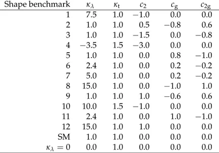
i.e. κλ =0. The values of these benchmark coupling parameters are given in Table 1.

Table 1: Parameter values of the couplings corresponding to the twelve shape benchmarks, the

SM prediction, and the case with vanishing Higgs boson self-interaction, κλ =0.

Shape benchmark κλ κt c2 cg c2g 1 7.5 1.0 −1.0 0.0 0.0 2 1.0 1.0 0.5 −0.8 0.6 3 1.0 1.0 −1.5 0.0 −0.8 4 −3.5 1.5 −3.0 0.0 0.0 5 1.0 1.0 0.0 0.8 −1.0 6 2.4 1.0 0.0 0.2 −0.2 7 5.0 1.0 0.0 0.2 −0.2 8 15.0 1.0 0.0 −1.0 1.0 9 1.0 1.0 1.0 −0.6 0.6 10 10.0 1.5 −1.0 0.0 0.0 11 2.4 1.0 0.0 1.0 −1.0 12 15.0 1.0 1.0 0.0 0.0 SM 1.0 1.0 0.0 0.0 0.0 κλ =0 0.0 1.0 0.0 0.0 0.0

The dominant background consists of events comprised uniquely of jets (multijet events) aris-ing from the SM quantum chromodynamics (QCD) interaction, and is modelled entirely from data. The remaining background, consisting mostly of tt+jets events, is less than 10% of the

total background, is modelled using POWHEG 2.0 [67–69] and interfaced to PYTHIA 8. The

CUETP8M2T4 tune [70, 71] is used for generating the tt+jets events. The tt+jets background

rate is estimated using a next-to-next-to-leading order cross section of 832+₋46₅₂pb [72],

corre-sponding to the top quark mass of 172.5 GeV. A sample of multijet events from QCD

inter-actions, simulated at leading order using MADGRAPH5 aMC@NLOand PYTHIA 8, is used to

develop and validate the background estimation techniques, prior to being applied to the data.

All generated samples were processed through a GEANT4-based [73, 74] simulation of the CMS

detector. The effect of pileup, averaging to 23 at the LHC beam conditions in 2016, is included in the simulations, and the samples are reweighted to match the distribution of the number of pp interactions observed in the data, assuming a total inelastic pp collision cross section of 69.2 mb [75].

4

Event selection

Five different HLT triggers were used to collect the semi-resolved events used in this analysis.

An event is selected if the scalar sum of the pT of all AK4 jets in the event (HT) is greater than

800 or 900 GeV, depending on the LHC beam instantaneous luminosity. Events with HT ≥

650 GeV, and a pair of jets with invariant mass above 900 GeV and a pseudorapidity separation

|∆η| < 1.5 are also selected. A third HLT trigger accepts events if the scalar sum of the pT of all AK8 jets is greater than 650 or 700 GeV and the “trimmed mass” of an AK8 jet is above 50 GeV. The jet trimmed mass is obtained after removing remnants of soft radiation with the jet

trimming technique [76], using a subjet size parameter of 0.3 and a subjet-to-AK8 jet pTfraction

of 0.1. Should an event contain an AK8 jet with pT >360 GeV and a trimmed mass greater than

30 GeV, it is selected by the fourth HLT trigger. Events containing two AK8 jets having pT >280

and 200 GeV, with at least one having trimmed mass greater than 30 GeV together with an AK4 jet passing a loose b-tagging criterion, pass the fifth HLT trigger.

Jets in events collected using the logical OR of the above HLT triggers are required to have

|η| <2.4, and pT >30 GeV for AK4 jets and pT >300 GeV for AK8 jets. One AK8 jet is used to

identify a boosted and spatially merged H→bb decay (H jets) while two AK4 jets are used to

reconstruct a spatially resolved H→bb decay.

The first H-tagging criterion requires an AK8 jet to have a soft-drop mass mJbetween 105 and

135 GeV, consistent with the measured mass of the Higgs boson mH =125 GeV. This selection

corresponds to an efficiency of about 60–70% for a resonant signal mass mXin the range 750–

3000 GeV. The soft-drop jet mass interval was chosen to include a large fraction of the boosted

H→ bb signal, while avoiding overlaps with CMS analyses searching for bulk gravitons and

radions decaying to boosted W and Z bosons [77]. The “N-subjettiness” algorithm [78] is used

on the AK8-PUPPI jet constituents, to compute the variables τN, which quantify the degree

to which a jet contains N subjets. A selection on the ratio τ21 ≡ τ2/τ1 < 0.55 is required for

all AK8 jets to be H tagged, which has a jet pT-dependent efficiency of 50–70%. The selection

criterion on τ21was optimized for signal sensitivity over the range of mXvalues explored.

A jet flavour requirement using a “double-b tagger” algorithm [79] is applied to the AK8 jet as the final H-tagging requirement. The double-b tagger is a multivariate discriminator with an output between -1 and 1, a higher value indicating a greater probability for the jet to contain a bb pair. The double-b tagger exploits the presence of two hadronized b quarks inside the

boosted H → bb decay, and uses variables related to b hadron lifetime and mass to

distin-guish H jets against a background of jets of other flavours. The double-b tagger algorithm also exploits the fact that the directions of the b hadron momentum are strongly correlated with

the axes used to calculate the N-subjettiness variables τN. An H jet candidate should have a

double-b tagger discriminator greater than 0.8, which corresponds to an efficiency of 30% and a misidentification rate of about 1%, as measured in a sample of multijet events. The efficiency of the double-b tagger for simulated jets is corrected to match that in the data, based on effi-ciency measurements using jets containing pairs of muons, thereby yielding samples enriched in jets from gluons splitting to bb pairs. These efficiency corrections are in between 0.92 and

1.02, for jets in the selected pT range.

To find a Higgs boson decay into two resolved b quark jets, all AK4 jets in each event are exam-ined for their b tag value using “DeepCSV” algorithm, which is a deep neural network, traexam-ined using information from tracks and secondary vertices associated to the jets [79]. The DeepCSV discriminator gives the probability of a jet to have originated from the hadronization of a bot-tom quark. A selection on the DeepCSV discriminator of AK4 jets is made, corresponding to a 1% mistag rate for light flavoured jets. The corresponding b-tagging efficiency is about 70% for

b quark jets in the pT range 80–150 GeV, and decreases to about 50% for pT∼1000 GeV. The b tagging efficiency in the simulations is corrected to match the one in the data, using measure-ments of the b tagging algorithm performance in a sample of muon-tagged jets and b jets from tt+jets events, where the correction factor ranges from approximately 0.95 to 1.1.

To identify events with a resolved H → bb decay, all pairs of b-tagged AK4 jet are examined,

to find events with at least one pair where each AK4 jet is at least∆R > 0.8 away from the

leading-pT AK8 jet and within ∆R < 1.5 of each other. If several such pairs are found, the

pair of jets, j₁ and j₂, that has the highest sum of the AK4 jet DeepCSV discriminator values is

selected. The leading-pTAK8 jet is then identified as the boosted H candidate, and the pair of

AK4 jets is identified as the resolved H candidate. If no pairs are found, this process is repeated

with the subleading-pTAK8 jet. If a pair of AK4 jets is identified, then the subleading-pT AK8

jet is identified as the boosted H candidate, and the pair of AK4 jets is identified as the resolved

H candidate. If no pairs are found once again, the event is rejected. The invariant mass of j₁

and j₂, mjj(j₁, j₂), is required to be within 90–140 GeV, forming the resolved H→bb candidate.

The tt+jets background is reduced by reconstructing a t →bqq system in events with three or

more AK4 jets, combining j₁ and j₂ with the nearest AK4 jet j₃. For the tt+jets background,

the trijet invariant mass mjjj(j₁, j₂, j₃) peaks around the top quark mass of 172 GeV. Hence,

mjjj(j₁, j₂, j₃)is required be greater than 200 GeV, namely above the top quark mass. Events

con-taining leptons (electrons or muons) with pT >20 GeV and|η| <2.4, and only a small amount

of energy in an area around the lepton direction compared to the lepton pT, are rejected, to

further suppress tt+jets and other backgrounds.

A resonant HH signal results in a small pseudorapidity separation between the two Higgs bosons, while the candidates from the multijet background typically have a larger pseudora-pidity separation. Events are therefore categorized according to the pseudorapseudora-pidity difference

between the H jet and the resolved H → bb candidate. These two categories are defined by

|_∆η(H jet, resolved H→bb)|within the interval 0.0–1.0 or within the interval 1.0–2.0.

To search for resonant and a non-resonant HH signals, the invariant mass distribution of the

boosted and resolved Higgs boson candidate system (mJjj) is examined for an excess of events

over the estimated background. The “reduced di-Higgs invariant mass” is defined as mJjj,red ≡

mJjj− (mJ−mH) − (mjj(j1, j2) −mH). The quantity mJjj,red is used rather than mJjjsince by sub-tracting the masses of the reconstructed H candidates and adding back the exact Higgs boson

mass mH, fluctuations from the jet mass resolution are corrected, leading to 8–10%

improve-ment in the HH mass resolution. After the full selection, the multijet background is about 90% of the total background, with the remaining background being tt+jets events.

With the above event selection, the trigger criteria reach an efficiency of greater than 99%

for events with mJjj,red ≥ 1100 GeV. For lower values of invariant mass (between 750 and

1100 GeV), the trigger efficiency is between 80 and 99% for 0≤ |∆η(H jet, resolved H→bb)| <

1 and between 60 and 99% for 1≤ |∆η(H jet, resolved H →bb)| ≤2. The trigger efficiency for

the data is estimated from a multijets sample collected with a control trigger requiring a single

AK4 jet with pT >260 GeV. The trigger efficiency for the simulated samples is corrected using

a scale factor to match the observed efficiency for the data. This scale factor depends mildly on

|∆η(H jet, resolved H→bb)|, and is hence applied as a function of this variable.

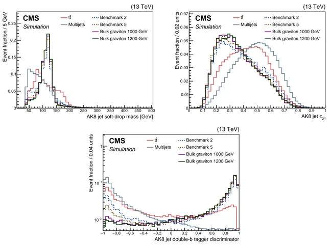
The AK8 jet soft-drop mass distribution, the N-subjettiness ratio τ21distribution, and the

double-b tagger discriminator distridouble-bution for the double-backgrounds and simulated signals are shown in Fig. 1. The DeepCSV discriminator distributions for the two AK4 jets, the dijet invariant mass distribution, and the trijet invariant mass distribution for the backgrounds and simulated

sam-AK8 jet soft-drop mass [GeV]

50 100 150 200 250 300 350 400 450 500

Event fraction / 5 GeV

0 0.05 0.1 0.15 0.2 0.25 t t Benchmark 2 Multijets Benchmark 5 Bulk graviton 1000 GeV Bulk graviton 1200 GeV

(13 TeV) CMS Simulation 21 τ AK8 jet 0 0.1 0.2 0.3 0.4 0.5 0.6 0.7 0.8 0.9 1

Event fraction / 0.02 units

0 0.01 0.02 0.03 0.04 0.05 0.06 0.07 t t Benchmark 2 Multijets Benchmark 5 Bulk graviton 1000 GeV Bulk graviton 1200 GeV

(13 TeV)

CMS Simulation

AK8 jet double-b tagger discriminator

1

− −0.8 −0.6 −0.4 −0.2 0 0.2 0.4 0.6 0.8 1

Event fraction / 0.04 units

2 − 10 1 − 10 1 t t Benchmark 2 Multijets Benchmark 5 Bulk graviton 1000 GeV Bulk graviton 1200 GeV

(13 TeV)

CMS Simulation

Figure 1: Distributions of the soft-drop mass (upper left), τ21 (upper right), and the

double-b tagger (lower), for AK8 jets in semi-resolved events. The multijet and the tt+jets double- back-ground components are shown separately, along with the simulated signals for bulk gravitons of masses 1000 and 1200 GeV and the non-resonant benchmark models 2 and 5. The distribu-tions are normalized to unity.

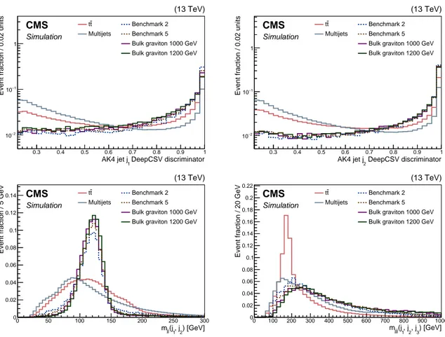
ples are shown in Fig. 2. The selection criteria for the above plots is as follows: AK8 jets with

pT >300 GeV, AK4 jets with pT >30 GeV, AK8 and AK4 jets with|η| < 2.4, AK8 jet soft-drop

mass> 40 GeV, AK4 jets DeepCSV discriminator> 0.2219,∆R < 1.5 separation between the

AK4 jets, and∆R>0.8 separation between the AK8 jet and each AK4 jet.

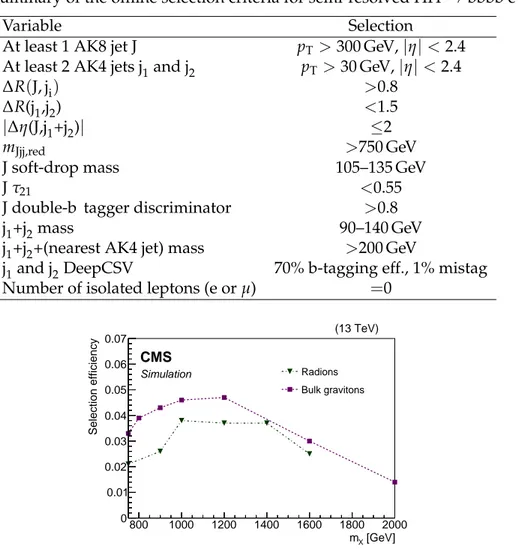
The semi-resolved event selection is summarized in Table 2, where in addition to these criteria, the events that are used by the fully-merged analysis of Ref. [39] are removed, as detailed at the end of this section. The event selection efficiencies for bulk gravitons and radions are given in Fig. 3, for different assumed masses in the range 750–2000 GeV. At low masses, the efficiency rise is mainly due to the increases in the trigger efficiency and in the efficiency of the

requirement on the|∆η|between the two Higgs boson candidates. The latter efficiency is more

important for the radion, which being a spin-0 particle has a wider |∆η|at low masses than

the spin-2 bulk graviton. At high masses, the efficiency drops because more events migrate to the fully-merged regime. The selection efficiencies for the non-resonant signals are between 0.01–2%.

In view of the statistical combination of the semi-resolved and the fully-merged analyses, we briefly describe the search in the fully-merged topology [39]. The analysis in the fully-merged regime uses the same trigger selection and the same selection for the H jet identification, except

DeepCSV discriminator

1

AK4 jet j

0.3 0.4 0.5 0.6 0.7 0.8 0.9 1

Event fraction / 0.02 units

2 − 10 1 − 10 1 t t Benchmark 2 Multijets Benchmark 5 Bulk graviton 1000 GeV Bulk graviton 1200 GeV

(13 TeV) CMS Simulation DeepCSV discriminator 2 AK4 jet j 0.3 0.4 0.5 0.6 0.7 0.8 0.9 1

Event fraction / 0.02 units

2 − 10 1 − 10 1 t t Benchmark 2 Multijets Benchmark 5 Bulk graviton 1000 GeV Bulk graviton 1200 GeV

(13 TeV) CMS Simulation ) [GeV] 2 , j 1 (j jj m 0 50 100 150 200 250 300

Event fraction / 5 GeV

0 0.02 0.04 0.06 0.08 0.1 0.12 0.14 tt Benchmark 2 Multijets Benchmark 5 Bulk graviton 1000 GeV Bulk graviton 1200 GeV

(13 TeV) CMS Simulation ) [GeV] 3 , j 2 , j 1 (j jjj m 0 100 200 300 400 500 600 700 800 900 1000

Event fraction / 20 GeV

0 0.02 0.04 0.06 0.08 0.1 0.12 0.14 0.16 0.18 0.2 0.22 t t Benchmark 2 Multijets Benchmark 5 Bulk graviton 1000 GeV Bulk graviton 1200 GeV

(13 TeV)

CMS Simulation

Figure 2: Distributions for AK4 jets of the DeepCSV discriminators for the leading j₁(upper left)

and next leading j₂(upper right), the invariant mass of j₁and j₂, mjj(j1, j2)(lower left), and the

invariant mass of j₁, j₂, and their nearest AK4 jet j₃, mJjj(j1, j2, j3)(lower right), in semi-resolved events. The multijet and tt+jets background components are shown separately, along with the simulated signals for bulk gravitons of masses 1000 and 1200 GeV and the non-resonant benchmark models 2 and 5. The distributions are normalized to unity.

instead of one. The fully-merged events are classified according to the values of the double-b

tagger discriminators of the two H jets, with both J₁ and J₂ required to pass a loose double-b

tagger discriminator value of> 0.3. Events are then categorized into those with both J₁ and

J₂ passing a tighter double-b tagger discriminator requirement of > 0.8, and the rest. The

pseudorapidity separation between J₁ and J₂is required to be |∆η(J₁, J₂)| < 1.3. The reduced

di-Higgs invariant mass for fully-merged events is defined as m_JJ,red = mJJ− (mJ1 −mH) −

(mJ2 −mH), where mJJ is the invariant mass of J1 and J2 and mJ1 and mJ2 are their soft-drop

masses, respectively.

A Higgs boson candidate which passes the boosted AK8 jet selection can also pass the selec-tion for two resolved AK4 jets. In particular, signal samples with higher mass that pass the semi-resolved selection often pass the fully-merged selection because both Higgs candidates are merged, but one candidate still passes the selection for a resolved jet as well. For each signal, the final semi-resolved selection includes anywhere from 23–53% events that are used by the fully-merged analysis, whether in the signal region or to estimate the QCD multijets background. These events are then removed from the semi-resolved analysis to allow for a combination with the fully-merged analysis.

Table 2: Summary of the offline selection criteria for semi-resolved HH→bbbb events.

Variable Selection

At least 1 AK8 jet J pT >300 GeV,|η| <2.4

At least 2 AK4 jets j₁and j₂ pT >30 GeV,|η| <2.4

∆R(J, j_i) >0.8

∆R(j₁,j₂) <1.5

|∆η(J,j₁+j₂)| ≤2

m_Jjj,red >750 GeV

J soft-drop mass 105–135 GeV

J τ21 <0.55

J double-b tagger discriminator >0.8

j₁+j₂mass 90–140 GeV

j₁+j₂+(nearest AK4 jet) mass >200 GeV

j₁and j₂DeepCSV 70% b-tagging eff., 1% mistag

Number of isolated leptons (e or µ) =0

[GeV] X m 800 1000 1200 1400 1600 1800 2000 Selection efficiency 0 0.01 0.02 0.03 0.04 0.05 0.06 0.07 Radions Bulk gravitons (13 TeV) CMS Simulation

Figure 3: The signal selection efficiencies for the radion and the bulk graviton, for different masses. The events are required to pass the selections given in Table 2 as well as to fail the selections of the fully-merged analysis of Ref. [39].

5

Background estimation

The multijet background estimation technique for the semi-resolved analysis is the same as that for the fully-merged analysis [39]. A set of signal-free control regions is defined by changing the criteria on the soft-drop mass and the double-b tagger discriminator of the selected AK8 jet from those used for the H tagging. The selection criteria applied to the AK4 jets forming

the resolved H→bb are the same as those used for the signal regions. If the soft-drop mass is

within 60 GeV above or below the H jet mass window of 105–135 GeV, these regions are referred to as the mass sideband regions. These sidebands are separated into regions that pass or fail the double-b tagger tagging requirement.

We define the pass-fail ratio Rp/fas the ratio of events for which the AK8 jet passes and fails the

double-b tagger tagging requirement. The Rp/f is measured in the soft-drop mass sidebands

as a function of soft-drop mass. These values are fit to a quadratic function of the H jet mass

to calculate the Rp/f in the signal region. The antitag region, defined with the same criteria as

the signal region, but with the AK8 jet failing the double-b tagger requirement, is then scaled

by the R_p/f value to estimate the multijets background in the signal region. This is done in

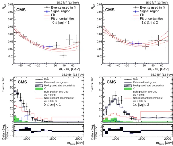
60 − −40 −20 0 20 40 60 [GeV] H m - J m 0 0.01 0.02 0.03 0.04 0.05 0.06 0.07 0.08 p/f

R Events used in fit

Signal region Fit Fit uncertainties | < 1 η ∆ | ≤ 0 (13 TeV) -1 35.9 fb CMS 60 − −40 −20 0 20 40 60 [GeV] H m - J m 0 0.01 0.02 0.03 0.04 0.05 0.06 0.07 0.08 p/f

R Events used in fit

Signal region Fit Fit uncertainties 2 ≤ | η ∆ | ≤ 1 (13 TeV) -1 35.9 fb CMS Events / bin 0 10 20 30 40 50 60 Data Estimated background Background stat. uncertainty

t t

Bulk graviton 800 GeV = 50 fb B σ Non-resonant benchmark 2 = 500 fb B σ [GeV] Jjj,red m 1000 1500 2000 Data unc. Data - Bkg. 2 − 0 2 (13 TeV) -1 35.9 fb CMS | < 1 η ∆ | ≤ 0 Events / bin 0 10 20 30 40 50 60 70 Data Estimated background Background stat. uncertainty

t t

Bulk graviton 800 GeV = 50 fb B σ Non-resonant benchmark 2 = 500 fb B σ [GeV] Jjj,red m 1000 1500 2000 Data unc. Data - Bkg. 2 − 0 2 (13 TeV) -1 35.9 fb CMS 2 ≤ | η ∆ | ≤ 1

Figure 4: Upper: The double-b tagger pass-fail ratio R_p/f of the leading-pT AK8 jet in

semi-resolved events as a function of the difference between the soft-drop mass and the Higgs boson

mass, mJ−mH. The measured ratio in different bins of mJ−mH is used in the fit (red solid

line), except in the region around mJ−mH = 0, which corresponds to the signal region (blue

markers). The fitted function is interpolated to obtain Rp/f in the signal region. Lower: The

reduced mass distribution mJjj,red in the data (black markers) with the estimated background

represented as the black histogram. The tt+jets contribution from simulation is represented in

green. The rest of the background is multijets, calculated by applying the Rp/f to the antitag

region. The uncertainty in the total background, before fitting the background model to the data, is depicted using the shaded region. The signal distributions for a bulk graviton with a mass of 800 GeV (blue) and the non-resonant benchmark 2 model (red) are also shown for assumed values of the products of the production cross sections for HH and the branching

fraction to 4b, σB. For the left and right figures, the pseudorapidity intervals are 0≤ |∆η| <1

and 1≤ |∆η| ≤2, respectively.

m_Jjj,red was found to be negligible, within the measurement uncertainties. Both the shape of

the background mJjj,reddistribution and its total yield in the signal region is obtained using this

method.

Prior to estimating the background, the tt+jets contributions derived from Monte Carlo simu-lation are subtracted from all sideband and signal regions in the data, and then added back in once the multijet background calculation is completed, to estimate the contribution of tt+jets to the total background. The fractions of signal events in the sideband regions were found to be negligible as compared with the total numbers of events.

Figure 4 (left) shows the quadratic fit in the AK8 jet soft-drop mass sidebands of the pass-fail

ratio Rp/fas a function of AK8 jet soft-drop mass, as obtained in the data and in the predicted

background shape in the signal region, where overlap with the merged analysis in the signal,

sideband, and antitag regions is removed. A χ2 _{test statistic was used to perform the fit, and}

the modelling was validated using Monte Carlo simulations and control samples in the data. The functional form was chosen after performing a Fisher F-test [80], which established that, among polynomials, a quadratic form is necessary and sufficient. Other functional forms were tested and the fit results were found to be consistent with that using the quadratic function. The resulting background distributions are compared with the observed data, as shown in Fig. 4 (right).

6

Systematic uncertainties

The following sources of systematic uncertainty affect the expected signal and background event yields. None of these lead to a significant change in the signal shape. A complete list of systematic uncertainties is given in Table 3.

Table 3: Summary of the ranges of systematic uncertainties in the signal and background yields, for both the semi-resolved analysis and for the fully-merged analysis, taken from Ref. [39].

Source Uncertainty (Semi-resolved) Uncertainty (Fully-merged)

Signal yield (%)

Trigger efficiency 1–15 1–15

Jet energy scale and resolution 1–3 1

Jet mass scale and resolution 2 2

H tagging correction factor 5–20 7–20

H jet τ21selection +14/-13 +30/-26

b tagging selection 2–9 2–5

PDF and scales 0.1–3 0.1–2

Pileup modelling 1–2 2

Luminosity 2.5 2.5

Trijet Invariant Mass 0.5 —

Background yield (%)

tt+jets cross section 5 —

QCD background R_p/ffit 2–10 2–7

The trigger response modelling uncertainties are particularly important for m_Jjj,red <1100 GeV,

where the trigger efficiency drops below 99%. The trigger efficiency data-to-simulations scale factor has an uncertainty between 1 and 15%, attributable to the control trigger inefficiency and the sample size used.

The impact of the jet energy scale and resolution uncertainties [54] on the signal yields was estimated to be 1–3%, depending on the signal mass. The jet mass scale and resolution, as well

as the τ21 selection efficiency data-to-simulation scale factors were measured using a sample

of boosted W → qq0 jets in semileptonic tt events. The jet mass scale and resolution has a 2%

effect on the signal yields because of a change in the mean of the H jet mass distribution. A

correction factor is applied to account for the difference in the jet shower profile of W→qq0and

HERWIG++ shower generators. This uncertainty, the H tagging correction factor, is in the range

5–20%, depending on the resonance mass mX. The τ21selection efficiency uncertainty depends

on how many τ21tags are used, two for the fully-merged (26–30% uncertainty) and one for the

semi-resolved analysis (13–15% uncertainty). This includes an additional uncertainty in the τ21

scale factor, determined using simulations, for jets with pT higher than those in the tt events

used for the evaluation of this systematic.

Scale factors are used to correct the signal events yields so their double-b tagger and DeepCSV discriminator efficiencies are the same as for data. The double-b tagger and the DeepCSV dis-criminator scale factors are taken to be 100% correlated. The associated uncertainty is 2–9% [79],

depending on the double-b tagger and requirement threshold and jet pT, and is propagated to

the total uncertainty in the signal yield.

The impact of the theoretical scale uncertainties and PDF uncertainties, the latter derived using the PDF4LHC procedure [60] and the NNPDF3.0 PDF sets, is estimated to be 0.1–3%. These un-certainties affect the product of the signal acceptance and the selection efficiency. The scale and

the PDF uncertainties have negligible impact on the signal mJjj,red distributions. Additional

systematic uncertainties associated with the pileup modelling (1–2%, based on a 4.6% varia-tion on the pp total inelastic cross secvaria-tion) and with the integrated luminosity determinavaria-tion (2.5%) [81], are applied to the signal yield.

The systematic uncertainty on the trijet invariant mass cut was calculated by comparing the cut efficiency for Pythia and Herwig bulk graviton samples, and is equivalent to a 0.5% systematic. The systematic uncertainty applied to the signal is also applied to the tt+jets background in the semi-resolved analysis, as appropriate. The total uncertainty in the tt+jets background is 11–15%, of which 6% derives from the uncertainty in the tt+jets cross section.

The main source of uncertainty for the multijet background is due to the statistical uncertainty

in the fit to the Rp/fratio performed in the H jet mass sidebands. This uncertainty, amounting

to 2–10%, is fully correlated between all mJjj,redbins. Additional statistical uncertainties on the

background shape and yield in the signal region result from the finite statistics of the multijets samples in the antitag region and are evaluated using the Barlow–Beeston Lite method [82,

83]. These uncertainties are small as compared with the uncertainty on the Rp/fratio, and are

uncorrelated from bin to bin.

7

Results

This analysis extends the search for a resonance X decaying to HH→ bbbb with two boosted

H jets [39] to cover the semi-resolved topology involving one boosted H jet and one resolved

H → bb decay reconstructed using two b jets. An HH signal would appear as an excess of

events over estimated background in the mJjj,redspectra of the different signal event categories,

as discussed in Section 5.

The binned mJjj,reddistributions of the signal and the background are fitted to the data, as shown

in Fig. 4 (right), and examined for an excess of events above the predicted background. The data were found to be consistent with the expected background predictions. Upper limits on the product of the signal cross sections and branching fractions are obtained using the pro-file likelihood as a test statistic [84]. The systematic uncertainties are treated as nuisance pa-rameters and are profiled in the minimization of the negative of the logarithm of the profile likelihood ratio and the distributions of the likelihood ratio are calculated using the asymp-totic approximation [85] of the procedure reported in Refs. [86, 87]. Upper limits at 95%

[GeV] X m 1000 1500 2000 2500 3000 ) [fb] b b b b → HH → (X B X) → (pp σ 1 − 10 1 10 2 10 3 10 4 10 5 10 6 10 _{95% CL upper limits} Observed Median expected 68% expected 95% expected = 0.5) Pl M / κ Bulk KK graviton ( (13 TeV) -1 35.9 fb CMS fully-merged Semi-resolved+ only Fully-merged [GeV] X m 1000 1500 2000 2500 3000 ) [fb] b b b b → HH → (X B X) → (pp σ 1 − 10 1 10 2 10 3 10 4 10 5 10 6 10 _{95% CL upper limits} Observed Median expected 68% expected 95% expected = 3000 GeV) R Λ Radion ( (13 TeV) -1 35.9 fb CMS fully-merged Semi-resolved+ only Fully-merged

Figure 5: The upper limits for a bulk graviton (left) and radion (right), combining the fully-merged and the semi-resolved analysis (where the events used in the fully-fully-merged analysis are not considered in the semi-resolved analysis). The inner (green) and the outer (yellow) bands indicate the regions containing the 68 and 95%, respectively, of the distribution of limits expected under the background-only hypothesis. The theoretical predictions are shown as the red lines. Results above 2000 (1600) GeV for the bulk graviton (radion) are taken directly from the fully-merged analysis [39].

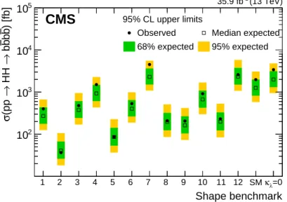
Shape benchmark 1 2 3 4 5 6 7 8 9 10 11 12 SMκ_λ=0 ) [fb] b b b b → HH → (pp σ 2 10 3 10 4 10 5 10 95% CL upper limits

Observed Median expected

68% expected 95% expected

CMS

(13 TeV)

-1

35.9 fb

Figure 6: The observed and expected upper limits for non-resonant HH production in the

stan-dard model, the model with κλ = 0, and other shape benchmarks (1–12), combining the

fully-merged selection and the semi-resolved selection (where the events used in the fully-fully-merged analysis are not considered in the semi-resolved analysis). The inner (green) and the outer (yel-low) bands indicate the regions containing the 68 and 95%, respectively, of the distribution of limits expected under the background-only hypothesis.

dence level are set on the product of the production cross section and the branching fractions

σ(pp→X)B(X→bbbb).

Results are obtained using a statistical combination of the semi-resolved and fully-merged event categories for the bulk graviton having a mass between 750–2000 GeV, and a radion with a mass between 750–1600 GeV. Above these mass ranges, the inclusion of the semi-resolved events does not appreciably improve the search sensitivity, as evidenced from the expected

limit values. The limits on σ(pp →X)B(X → bbbb)are shown in Fig. 5, and tabulated in

Ta-bles 4 and 5 for the bulk graviton and the radion, respectively. The limits for mX >2000 GeV for

the bulk graviton, and mX > 1600 GeV for the radion are those from the fully-merged analysis

of Ref. [39].

For the interpretation of the results, this paper uses the scenario of Ref. [88] to describe a KK graviton, where the propagation of SM fields is allowed in the bulk, and follows the character-istics of the SM gauge group, with the right-handed top quark localized near the TeV brane. The radion is an additional element of WED models that is needed to stabilize the size of the

extra dimension l. The theoretical cross sections for σ(pp → X)B(X → bbbb)are calculated

using κ/M_Pl = 0.5 for the bulk gravitons andΛR =3 TeV for the radions, of different masses.

For these values of κ/M_PlandΛR, the branching fractionsB(X → bbbb)are 10 and 23%, for

the graviton and the radion, respectively [89]. As shown in Fig. 5 (right), a radion having a

mass between 1000 and 1500 GeV is excluded at 95% confidence level forΛR =3 TeV.

The improvement in the upper limits on σ(pp → X)B(X → bbbb) due to the inclusion of

the semi-resolved event category between 18% and 7%, for a bulk graviton in the mass range 750–2000 GeV. A much larger improvement—between 55% and 8%—is seen for a radion in the

mass range 750–1600 GeV. This can be attributed to the two pseudorapidity intervals,|∆η| <1

and 1≤ |_∆η| ≤2, utilized in the semi-resolved event selection, with the lower pseudorapidity

interval having a better signal to background ratio for a spin-0 radion, because of the angular distribution of its decay products.

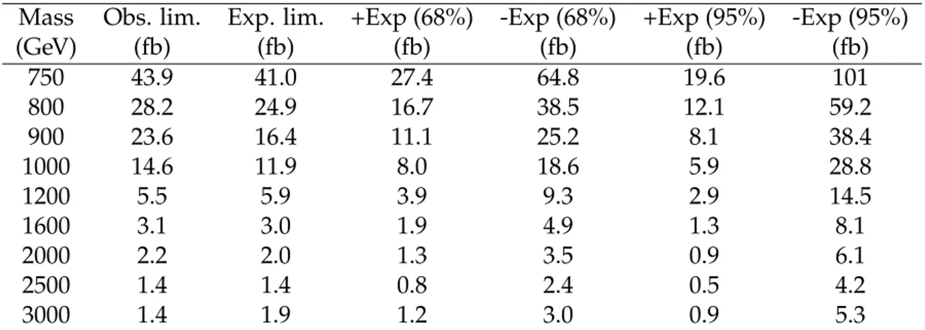
Table 4: The observed and expected upper limits on the products of the cross sections and

branching fraction σ(pp→ X)B(X→ HH →bbbb)for a bulk graviton from the combination

of the fully-merged and semi-resolved channels (where the events used in the fully-merged analysis are not considered in the semi-resolved analysis). Results above 2000 GeV are taken directly from the fully-merged analysis [39].

Mass Obs. lim. Exp. lim. +Exp (68%) -Exp (68%) +Exp (95%) -Exp (95%)

(GeV) (fb) (fb) (fb) (fb) (fb) (fb) 750 43.9 41.0 27.4 64.8 19.6 101 800 28.2 24.9 16.7 38.5 12.1 59.2 900 23.6 16.4 11.1 25.2 8.1 38.4 1000 14.6 11.9 8.0 18.6 5.9 28.8 1200 5.5 5.9 3.9 9.3 2.9 14.5 1600 3.1 3.0 1.9 4.9 1.3 8.1 2000 2.2 2.0 1.3 3.5 0.9 6.1 2500 1.4 1.4 0.8 2.4 0.5 4.2 3000 1.4 1.9 1.2 3.0 0.9 5.3

In addition, both the fully-merged and the semi-resolved analyses look for non-resonant HH production. The observed and expected upper limits are presented in Table 6 for the semi-resolved and the fully-merged signal categories combined, also depicted in Fig. 6. The observed and expected limits are respectively, 179 and 114 times the product of the SM cross sections and branching fractions. The new limits are better by about a factor of three for benchmark 2 and a factor of two for benchmark 5, with significant improvements for benchmarks 8, 9, and 11, compared to existing measurements [36, 38]. The increased sensitivity of this analysis to certain benchmarks is due to the higher level of destructive interference among the HH production processes close to the kinematic threshold, which leads to a corresponding shift of

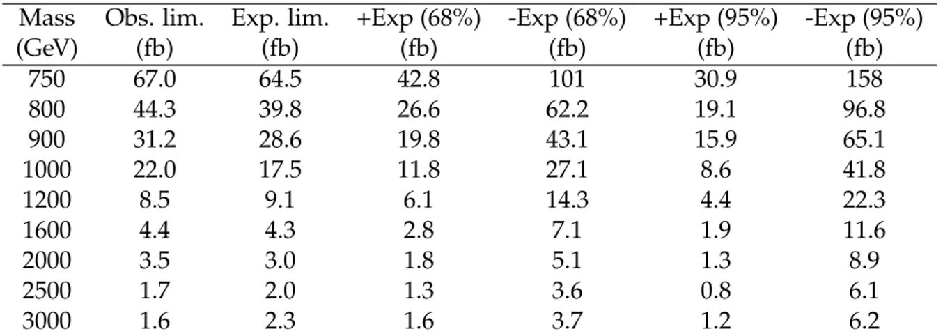
Table 5: The observed and expected upper limits on the products of the cross sections and

branching fraction σ(pp→ X)B(X → HH → bbbb)for a radion from the combination of the

fully-merged and semi-resolved channels (where the events used in the fully-merged analysis are not considered in the semi-resolved analysis). Results above 1600 GeV for the radion are taken directly from the fully-merged analysis [39].

Mass Obs. lim. Exp. lim. +Exp (68%) -Exp (68%) +Exp (95%) -Exp (95%)

(GeV) (fb) (fb) (fb) (fb) (fb) (fb) 750 67.0 64.5 42.8 101 30.9 158 800 44.3 39.8 26.6 62.2 19.1 96.8 900 31.2 28.6 19.8 43.1 15.9 65.1 1000 22.0 17.5 11.8 27.1 8.6 41.8 1200 8.5 9.1 6.1 14.3 4.4 22.3 1600 4.4 4.3 2.8 7.1 1.9 11.6 2000 3.5 3.0 1.8 5.1 1.3 8.9 2500 1.7 2.0 1.3 3.6 0.8 6.1 3000 1.6 2.3 1.6 3.7 1.2 6.2

Table 6: The observed and expected upper limits on the cross section σ(pp → HH → bbbb)

for the non-resonant shape benchmark models (1–12), the SM, and the κλ = 0 HH

produc-tions, combining merged and semi-resolved channels (where the events used in the fully-merged analysis are not considered in the semi-resolved analysis).

Shape Obs. lim. Exp. lim. +Exp (68%) -Exp (68%) +Exp (95%) -Exp (95%)

benchmark (fb) (fb) (fb) (fb) (fb) (fb) 1 401 271 179 428 127 660 2 36.7 41.0 26.5 66.3 18.5 105 3 479 376 247 601 173 936 4 1510 932 618 1460 438 2240 5 86.6 85.9 54.4 140 37.0 225 6 533 403 268 637 190 978 7 4520 2300 1530 3580 1100 5470 8 209 196 126 317 87.2 504 9 206 163 106 264 74 415 10 916 670 433 1070 302 1660 11 232 198 125 326 85.9 526 12 2600 2330 1530 3700 1090 5750 SM 1980 1260 833 1970 589 3030 κλ =0 3404 1989 3092 1334 4732 960

Higgs bosons, and hence in the sensitivity of this analysis, which identifies Higgs bosons using boosted techniques.

8

Summary

A search is presented for the pair production of standard model Higgs bosons (HH), both decaying to a bottom quark-antiquark pair (bb), using data from proton-proton collisions at

a centre-of-mass energy of 13 TeV and corresponding to an integrated luminosity of 35.9 fb−1.

a large Lorentz boost, so that the H→bb decay products are collimated to form a single jet, an H jet. The search combines events with one H jet plus two b jets with events having two H jets, thus adding sensitivity to the previous analysis [39].

The results of the search are compared with predictions for the resonant production of a nar-row Kaluza–Klein bulk graviton and a narnar-row radion in warped extradimensional models. The search is also sensitive to several beyond standard model non-resonant HH production scenar-ios. Such cases may arise either when an off-shell massive resonance produced in proton-proton collisions decays to HH, or through beyond standard model effects in the Higgs boson coupling parameters. The results are interpreted in terms of upper limits on the product of the

cross section for the respective signal processes and the branching fraction to HH → bbbb, at

95% confidence level.

The upper limits range from 43.9 to 1.4 fb for the bulk graviton and from 67 to 1.6 fb for the radion for the mass range 750–3000 GeV. Depending on the mass of the resonance, these limits improve upon the results of Ref. [39] by up to 18% for the bulk graviton and up to 55% for the radion.

The non-resonant production of Higgs boson pairs is modelled using an effective Lagrangian with five coupling parameters. The upper limit corresponding to the standard model values of the coupling parameters is placed at 1980 fb, which is 179 times the prediction. In addition, up-per limits in the range of 4520 to 36.7 fb are set on twelve shape benchmarks, i.e. representative sets of the five coupling parameters [66]. These are the first limits on non-resonant Higgs boson pair-production signals using boosted topologies, and are the most stringent limits to date for the shape benchmarks 2, 5, 8, 9, and 11.

Acknowledgments

We congratulate our colleagues in the CERN accelerator departments for the excellent perfor-mance of the LHC and thank the technical and administrative staffs at CERN and at other CMS institutes for their contributions to the success of the CMS effort. In addition, we gratefully acknowledge the computing centres and personnel of the Worldwide LHC Computing Grid for delivering so effectively the computing infrastructure essential to our analyses. Finally, we acknowledge the enduring support for the construction and operation of the LHC and the CMS detector provided by the following funding agencies: BMBWF and FWF (Austria); FNRS and FWO (Belgium); CNPq, CAPES, FAPERJ, FAPERGS, and FAPESP (Brazil); MES (Bulgaria); CERN; CAS, MoST, and NSFC (China); COLCIENCIAS (Colombia); MSES and CSF (Croa-tia); RPF (Cyprus); SENESCYT (Ecuador); MoER, ERC IUT, and ERDF (Estonia); Academy of Finland, MEC, and HIP (Finland); CEA and CNRS/IN2P3 (France); BMBF, DFG, and HGF (Germany); GSRT (Greece); NKFIA (Hungary); DAE and DST (India); IPM (Iran); SFI (Ireland); INFN (Italy); MSIP and NRF (Republic of Korea); MES (Latvia); LAS (Lithuania); MOE and UM (Malaysia); BUAP, CINVESTAV, CONACYT, LNS, SEP, and UASLP-FAI (Mexico); MOS (Mon-tenegro); MBIE (New Zealand); PAEC (Pakistan); MSHE and NSC (Poland); FCT (Portugal); JINR (Dubna); MON, RosAtom, RAS, RFBR, and NRC KI (Russia); MESTD (Serbia); SEIDI, CPAN, PCTI, and FEDER (Spain); MOSTR (Sri Lanka); Swiss Funding Agencies (Switzerland); MST (Taipei); ThEPCenter, IPST, STAR, and NSTDA (Thailand); TUBITAK and TAEK (Turkey); NASU and SFFR (Ukraine); STFC (United Kingdom); DOE and NSF (USA).

Individuals have received support from the Marie-Curie programme and the European Re-search Council and Horizon 2020 Grant, contract No. 675440 (European Union); the Leventis Foundation; the A. P. Sloan Foundation; the Alexander von Humboldt Foundation; the Belgian

Federal Science Policy Office; the Fonds pour la Formation `a la Recherche dans l’Industrie et dans l’Agriculture (FRIA-Belgium); the Agentschap voor Innovatie door Wetenschap en Tech-nologie (IWT-Belgium); the F.R.S.-FNRS and FWO (Belgium) under the “Excellence of Science - EOS” - be.h project n. 30820817; the Ministry of Education, Youth and Sports (MEYS) of the Czech Republic; the Lend ¨ulet (“Momentum”) Programme and the J´anos Bolyai Research

Schol-arship of the Hungarian Academy of Sciences, the New National Excellence Program ´UNKP,

the NKFIA research grants 123842, 123959, 124845, 124850 and 125105 (Hungary); the Council of Science and Industrial Research, India; the HOMING PLUS programme of the Foundation for Polish Science, cofinanced from European Union, Regional Development Fund, the Mo-bility Plus programme of the Ministry of Science and Higher Education, the National Science Center (Poland), contracts Harmonia 2014/14/M/ST2/00428, Opus 2014/13/B/ST2/02543, 2014/15/B/ST2/03998, and 2015/19/B/ST2/02861, Sonata-bis 2012/07/E/ST2/01406; the National Priorities Research Program by Qatar National Research Fund; the Programa Estatal de Fomento de la Investigaci ´on Cient´ıfica y T´ecnica de Excelencia Mar´ıa de Maeztu, grant MDM-2015-0509 and the Programa Severo Ochoa del Principado de Asturias; the Thalis and Aristeia programmes cofinanced by EU-ESF and the Greek NSRF; the Rachadapisek Sompot Fund for Postdoctoral Fellowship, Chulalongkorn University and the Chulalongkorn Aca-demic into Its 2nd Century Project Advancement Project (Thailand); the Welch Foundation, contract C-1845; and the Weston Havens Foundation (USA).

References

[1] ATLAS Collaboration, “Observation of a new particle in the search for the standard model Higgs boson with the ATLAS detector at the LHC”, Phys. Lett. B 716 (2012) 01,

doi:10.1016/j.physletb.2012.08.020, arXiv:1207.7214.

[2] CMS Collaboration, “Observation of a new boson at a mass of 125 GeV with the CMS experiment at the LHC”, Phys. Lett. B 716 (2012) 30,

doi:10.1016/j.physletb.2012.08.021, arXiv:1207.7235.

[3] CMS Collaboration, “Observation of a new boson with mass near 125 GeV in pp

collisions at√s = 7 and 8 TeV”, JHEP 06 (2013) 081,

doi:10.1007/JHEP06(2013)081, arXiv:1303.4571.

[4] D. de Florian et al., “Handbook of LHC Higgs cross sections: 4. deciphering the nature of the Higgs sector”, CERN Report CERN-2017-002-M, 2016.

doi:10.23731/CYRM-2017-002, arXiv:1610.07922.

[5] D. de Florian and J. Mazzitelli, “Higgs boson pair production at next-to-next-to-leading order in QCD”, Phys. Rev. Lett. 111 (2013) 201801,

doi:10.1103/PhysRevLett.111.201801, arXiv:1309.6594.

[6] J. Baglio et al., “The measurement of the Higgs self-coupling at the LHC: theoretical status”, JHEP 04 (2013) 151, doi:10.1007/JHEP04(2013)151, arXiv:1212.5581. [7] L. Randall and R. Sundrum, “A large mass hierarchy from a small extra dimension”,

Phys. Rev. Lett. 83 (1999) 3370, doi:10.1103/PhysRevLett.83.3370,

arXiv:hep-ph/9905221.

[8] R. Grober and M. Muhlleitner, “Composite Higgs boson pair production at the LHC”, JHEP 06 (2011) 020, doi:10.1007/JHEP06(2011)020, arXiv:1012.1562.

[9] W. D. Goldberger and M. B. Wise, “Modulus stabilization with bulk fields”, Phys. Rev. Lett. 83 (1999) 4922, doi:10.1103/PhysRevLett.83.4922,

arXiv:hep-ph/9907447.

[10] O. DeWolfe, D. Z. Freedman, S. S. Gubser, and A. Karch, “Modeling the fifth dimension with scalars and gravity”, Phys. Rev. D 62 (2000) 046008,

doi:10.1103/PhysRevD.62.046008, arXiv:hep-th/9909134.

[11] C. Csaki, M. Graesser, L. Randall, and J. Terning, “Cosmology of brane models with radion stabilization”, Phys. Rev. D 62 (2000) 045015,

doi:10.1103/PhysRevD.62.045015, arXiv:hep-ph/9911406.

[12] H. Davoudiasl, J. L. Hewett, and T. G. Rizzo, “Phenomenology of the Randall-Sundrum gauge hierarchy model”, Phys. Rev. Lett. 84 (2000) 2080,

doi:10.1103/PhysRevLett.84.2080, arXiv:hep-ph/9909255.

[13] C. Csaki, M. L. Graesser, and G. D. Kribs, “Radion dynamics and electroweak physics”, Phys. Rev. D 63 (2001) 065002, doi:10.1103/PhysRevD.63.065002,

arXiv:hep-th/0008151.

[14] K. Agashe, H. Davoudiasl, G. Perez, and A. Soni, “Warped gravitons at the LHC and beyond”, Phys. Rev. D 76 (2007) 036006, doi:10.1103/PhysRevD.76.036006,

arXiv:hep-ph/0701186.

[15] G. F. Giudice, R. Rattazzi, and J. D. Wells, “Graviscalars from higher dimensional metrics and curvature Higgs mixing”, Nucl. Phys. B 595 (2001) 250,

doi:10.1016/S0550-3213(00)00686-6, arXiv:hep-ph/0002178.

[16] S. Dawson, A. Ismail, and I. Low, “What’s in the loop? The anatomy of double Higgs production”, Phys. Rev. D 91 (2015) 115008, doi:10.1103/PhysRevD.91.115008,

arXiv:1504.05596.

[17] ATLAS and CMS Collaborations, “Combined measurement of the Higgs boson mass in

pp collisions at√s =7 and 8 TeV with the ATLAS and CMS experiments”, Phys. Rev.

Lett. 114 (2015) 191803, doi:10.1103/PhysRevLett.114.191803,

arXiv:1503.07589.

[18] CMS Collaboration, “Measurements of properties of the Higgs boson decaying into the

four-lepton final state in pp collisions at√s=13 TeV”, JHEP 11 (2017) 047,

doi:10.1007/JHEP11(2017)047, arXiv:1706.09936.

[19] G. F. Giudice, C. Grojean, A. Pomarol, and R. Rattazzi, “The strongly-interacting light Higgs”, JHEP 06 (2007) 045, doi:10.1088/1126-6708/2007/06/045,

arXiv:hep-ph/0703164.

[20] CMS Collaboration, “Precise determination of the mass of the Higgs boson and tests of compatibility of its couplings with the standard model predictions using proton

collisions at 7 and 8 TeV”, Eur. Phys. J. C 75 (2015) 212,

doi:10.1140/epjc/s10052-015-3351-7, arXiv:1412.8662.

[21] ATLAS Collaboration, “Measurements of the Higgs boson production and decay rates

and coupling strengths using pp collision data at√s=7 and 8 TeV in the ATLAS

experiment”, Eur. Phys. J. C 76 (2016) 6, doi:10.1140/epjc/s10052-015-3769-y,

[22] ATLAS Collaboration, “Search for Higgs boson pair production in the γγbb final state

using pp collision data at√s =8 TeV from the ATLAS detector”, Phys. Rev. Lett. 114

(2015) 081802, doi:10.1103/PhysRevLett.114.081802, arXiv:1406.5053. [23] ATLAS Collaboration, “Search for Higgs boson pair production in the bbbb final state

from pp collisions at√s =8 TeV with the ATLAS detector”, Eur. Phys. J. C 75 (2015) 412,

doi:10.1140/epjc/s10052-015-3628-x, arXiv:1506.00285.

[24] ATLAS Collaboration, “Searches for Higgs boson pair production in the HH→bbττ,

γγWW∗, γγbb, bbbb channels with the ATLAS detector”, Phys. Rev. D 92 (2015) 092004,

doi:10.1103/PhysRevD.92.092004, arXiv:1509.04670.

[25] ATLAS Collaboration, “Search for pair production of Higgs bosons in the bbbb final state

using proton–proton collisions at√s=13 TeV with the ATLAS detector”, Phys. Rev. D

94(2016) 052002, doi:10.1103/PhysRevD.94.052002, arXiv:1606.04782.

[26] ATLAS Collaboration, “Search for pair production of Higgs bosons in the bbbb final state

using proton-proton collisions at√s=13 TeV with the ATLAS detector”, (2018).

arXiv:1804.06174.

[27] ATLAS Collaboration, “Search for Resonant and Nonresonant Higgs Boson Pair

Production in the bbτ+τ−Decay Channel in pp Collisions at

√

s=13 TeV with the

ATLAS Detector”, Phys. Rev. Lett. 121 (2018) 191801,

doi:10.1103/PhysRevLett.121.191801, arXiv:1808.00336.

[28] ATLAS Collaboration, “Search for Higgs boson pair production in the γγWW∗channel

using pp collision data recorded at√s=13 TeV with the ATLAS detector”, (2018).

arXiv:1807.08567. Submitted to Eur. Phys. J. C.

[29] ATLAS Collaboration, “Search for Higgs boson pair production in the γγbb final state with 13 TeV pp collision data collected by the ATLAS experiment”, JHEP 11 (2018) 040,

doi:10.1007/JHEP11(2018)040, arXiv:1807.04873.

[30] CMS Collaboration, “Searches for heavy Higgs bosons in two-Higgs-doublet models and

for t→ch decay using multilepton and diphoton final states in pp collisions at 8 TeV”,

Phys. Rev. D 90 (2014) 112013, doi:10.1103/PhysRevD.90.112013,

arXiv:1410.2751.

[31] CMS Collaboration, “Search for Higgs boson pair production in the bbττ final state in

proton-proton collisions at√s=8 TeV”, Phys. Rev. D 96 (2017) 072004,

doi:10.1103/PhysRevD.96.072004, arXiv:1707.00350.

[32] CMS Collaboration, “Search for resonant pair production of Higgs bosons decaying to two bottom quark-antiquark pairs in proton-proton collisions at 8 TeV”, Phys. Lett. B 749 (2015) 560, doi:10.1016/j.physletb.2015.08.047, arXiv:1503.04114.

[33] CMS Collaboration, “Searches for a heavy scalar boson H decaying to a pair of 125 GeV Higgs bosons hh or for a heavy pseudoscalar boson A decaying to Zh, in the final states

with h→ττ”, Phys. Lett. B 755 (2016) 217,

doi:10.1016/j.physletb.2016.01.056, arXiv:1510.01181.

[34] CMS Collaboration, “Search for two Higgs bosons in final states containing two photons and two bottom quarks in proton-proton collisions at 8 TeV”, Phys. Rev. D 94 (2016) 052012, doi:10.1103/PhysRevD.94.052012, arXiv:1603.06896.

[35] CMS Collaboration, “Search for heavy resonances decaying to two Higgs bosons in final states containing four b quarks”, Eur. Phys. J. C 76 (2016) 371,

doi:10.1140/epjc/s10052-016-4206-6, arXiv:1602.08762.

[36] CMS Collaboration, “Search for Higgs boson pair production in events with two bottom

quarks and two tau leptons in proton-proton collisions at√s=13 TeV”, Phys. Lett. B 778

(2018) 101, doi:10.1016/j.physletb.2018.01.001, arXiv:1707.02909. [37] CMS Collaboration, “Search for resonant and nonresonant Higgs boson pair production

in the bb`ν`νfinal state in proton-proton collisions at

√

s=13 TeV”, JHEP 01 (2018) 054,

doi:10.1007/JHEP01(2018)054, arXiv:1708.04188.

[38] CMS Collaboration, “Search for Higgs boson pair production in the γγbb final state in pp

collisions at√s=13 TeV”, Phys. Lett. B 788 (2019) 7,

doi:10.1016/j.physletb.2018.10.056, arXiv:1806.00408.

[39] CMS Collaboration, “Search for a massive resonance decaying to a pair of Higgs bosons

in the four b quark final state in proton-proton collisions at√s=13 TeV”, Phys. Lett. B

781(2018) 244, doi:10.1016/j.physletb.2018.03.084, arXiv:1710.04960.

[40] CMS Collaboration, “Search for resonant pair production of Higgs bosons decaying to bottom quark-antiquark pairs in proton-proton collisions at 13 TeV”, JHEP 08 (2018) 152, doi:10.1007/JHEP08(2018)152, arXiv:1806.03548.

[41] M. Gouzevitch et al., “Scale-invariant resonance tagging in multijet events and new physics in Higgs pair production”, JHEP 07 (2013) 148,

doi:10.1007/JHEP07(2013)148, arXiv:1303.6636.

[42] CMS Collaboration, “The CMS experiment at the CERN LHC”, JINST 3 (2008) S08004,

doi:10.1088/1748-0221/3/08/S08004.

[43] CMS Collaboration, “The CMS trigger system”, JINST 12 (2017) P01020,

doi:10.1088/1748-0221/12/01/P01020, arXiv:1609.02366.

[44] CMS Collaboration, “Particle-flow reconstruction and global event description with the CMS detector”, JINST 12 (2017) P10003, doi:10.1088/1748-0221/12/10/P10003, arXiv:1706.04965.

[45] M. Cacciari, G. P. Salam, and G. Soyez, “The anti-kTjet clustering algorithm”, JHEP 04

(2008) 063, doi:10.1088/1126-6708/2008/04/063, arXiv:0802.1189.

[46] M. Cacciari, G. P. Salam, and G. Soyez, “FastJet user manual”, Eur. Phys. J. C 72 (2012) 1896, doi:10.1140/epjc/s10052-012-1896-2, arXiv:1111.6097.

[47] M. Cacciari and G. P. Salam, “Pileup subtraction using jet areas”, Phys. Lett. B 659 (2008) 119, doi:10.1016/j.physletb.2007.09.077, arXiv:0707.1378.

[48] CMS Collaboration, “Jet energy scale and resolution in the CMS experiment in pp collisions at 8 TeV”, JINST 12 (2017) P02014,

doi:10.1088/1748-0221/12/02/P02014, arXiv:1607.03663.

[49] CMS Collaboration, “Jet energy scale and resolution performances with 13 TeV data”, CMS Detector Performance Summary CMS-DP-2016-020, CERN, 2016.

[50] D. Bertolini, P. Harris, M. Low, and N. Tran, “Pileup per particle identification”, JHEP 10 (2014) 059, doi:10.1007/JHEP10(2014)059, arXiv:1407.6013.

[51] G. P. Salam, “Towards jetography”, Eur. Phys. J. C 67 (2010) 637,

doi:10.1140/epjc/s10052-010-1314-6, arXiv:0906.1833.

[52] M. Dasgupta, A. Fregoso, S. Marzani, and G. P. Salam, “Towards an understanding of jet substructure”, JHEP 09 (2013) 029, doi:10.1007/JHEP09(2013)029,

arXiv:1307.0007.

[53] A. J. Larkoski, S. Marzani, G. Soyez, and J. Thaler, “Soft drop”, JHEP 05 (2014) 146, doi:10.1007/JHEP05(2014)146, arXiv:1402.2657.

[54] CMS Collaboration, “Jet algorithms performance in 13 TeV data”, CMS Physics Analysis Summary CMS-PAS-JME-16-003, CERN, 2017.

[55] J. Alwall et al., “The automated computation of tree-level and next-to-leading order differential cross sections, and their matching to parton shower simulations”, JHEP 07 (2014) 079, doi:10.1007/JHEP07(2014)079, arXiv:1405.0301.

[56] NNPDF Collaboration, “Parton distributions for the LHC Run II”, JHEP 04 (2015) 040,

doi:10.1007/JHEP04(2015)040, arXiv:1410.8849.

[57] L. A. Harland-Lang, A. D. Martin, P. Motylinski, and R. S. Thorne, “Parton distributions in the LHC era: MMHT 2014 PDFs”, Eur. Phys. J. C 75 (2015) 204,

doi:10.1140/epjc/s10052-015-3397-6, arXiv:1412.3989.

[58] A. Buckley et al., “LHAPDF6: parton density access in the LHC precision era”, Eur. Phys. J. C 75 (2015) 132, doi:10.1140/epjc/s10052-015-3318-8, arXiv:1412.7420. [59] S. Carrazza, J. I. Latorre, J. Rojo, and G. Watt, “A compression algorithm for the

combination of PDF sets”, Eur. Phys. J. C 75 (2015) 474,

doi:10.1140/epjc/s10052-015-3703-3, arXiv:1504.06469.

[60] J. Butterworth et al., “PDF4LHC recommendations for LHC Run II”, J. Phys. G 43 (2016) 023001, doi:10.1088/0954-3899/43/2/023001, arXiv:1510.03865.

[61] T. Sj ¨ostrand et al., “An Introduction to PYTHIA 8.2”, Comput. Phys. Commun. 191 (2015) 159, doi:10.1016/j.cpc.2015.01.024, arXiv:1410.3012.

[62] M. B¨ahr et al., “Herwig++ physics and manual”, Eur. Phys. J. C 58 (2008) 639,

doi:10.1140/epjc/s10052-008-0798-9, arXiv:0803.0883.

[63] CMS Collaboration, “Event generator tunes obtained from underlying event and multiparton scattering measurements”, Eur. Phys. J. C 76 (2016) 155,

doi:10.1140/epjc/s10052-016-3988-x, arXiv:1512.00815.

[64] S. Gieseke, C. Rohr, and A. Siodmok, “Colour reconnections in Herwig++”, Eur. Phys. J. C 72 (2012) 2225, doi:10.1140/epjc/s10052-012-2225-5, arXiv:1206.0041. [65] A. Carvalho et al., “Analytical parametrization and shape classification of anomalous HH

production in the EFT approach”, (2016). arXiv:1608.06578.

[66] A. Carvalho et al., “Higgs pair production: choosing benchmarks with cluster analysis”, JHEP 04 (2016) 126, doi:10.1007/JHEP04(2016)126.