See discussions, stats, and author profiles for this publication at: https://www.researchgate.net/publication/224254322
Model-in-the-loop development for fuel cell
vehicle
Conference Paper in Proceedings of the American Control Conference · August 2011 DOI: 10.1109/ACC.2011.5991604 · Source: IEEE Xplore CITATIONS5
READS191
3 authors, including: Melih Cakmakci Bilkent University 25 PUBLICATIONS 79 CITATIONS SEE PROFILE Shuzhen Liu Ford Motor Company 1 PUBLICATION 5 CITATIONS SEE PROFILEAll content following this page was uploaded by Melih Cakmakci on 07 July 2015. The user has requested enhancement of the downloaded file.
Abstract— In this paper, the work on developing and
validating a model-in-the-loop (MIL) simulation environment for a group of prototype fuel cell vehicles is presented. The MIL model consists of a vehicle plant model and an integrated vehicle system controller model. First, the vehicle simulation plant model is functionally validated with a simple vehicle system controller (VSC) model and then improved to satisfy the input output interface and fidelity requirements. The developed MIL system is then verified for basic functionality against the simple VSC controller model and shows uniform correlation results. It is further validated against vehicle dynamometer test data and demonstrates satisfactory consistency. A rapid model building approach which is suitable for model-based controller design process was also discussed. This approach enabled the developers to use model-to-code algorithms unlike many comparable simulation models.
I. INTRODUCTION
Increasing environmental concerns and awareness of the fact that fossil fuel will be depleted in the not long distant future have led to the rapid development of hybrid, fuel cell and battery electric vehicles in the past decade. Fuel cell technology has been considered the most promising alternative to substitute internal combustion engine for its zero emission characteristics and efficient use of renewable fuels. In the area of fuel cell vehicle (FCV) development, Ford Motor Company has been a technology leader [1]. Ford's Focus vehicle based technology demonstration FCV fleet has been operated by various partners around the globe for over five years and it has accumulated more than one million miles in total.
The fuel cell vehicle considered in this paper is a type of hybrid electric vehicle, based on Ford Explorer. In the following, it will be referred to as new generation FCV (NGFCV). The NGFCV has a primary power source, the fuel cell (which is controlled by the fuel cell control unit (FCU)), a secondary power source, the battery (which is controlled by the battery control module (BCM)), and a high voltage energy converter (HVEC) which converts DC/DC current between the battery bus and vehicle bus. Propulsion is achieved through the IPT (Integrated Power Train, or the drive motor) connected to the wheels (front, rear or all-wheel drive).
Melih Çakmakcı is with Bilkent University, Department of Mechanical Engineering, Ankara, 06800 Turkey (phone:+90-312-2903427; fax:+90-312-2664126; e-mail: [email protected]).
Yonghua Li is with the Vehicle and Battery Controls Department, Ford Motor Company, Dearborn, MI, 48121, USA (e-mail: [email protected]).
Shuzhen Liu is with the Model-Based Systems Engineering Department, Ford Motor Company, Dearborn, MI, 48121, USA (e-mail:
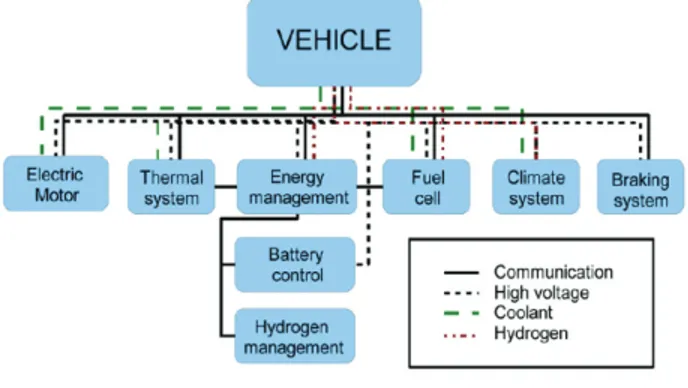
The architecture of the FCV considered in this paper is similar to the one given in [2] and summarized in Figure 1.
Figure 1 Fuel Cell Vehicle Architecture
In the FCV, a number of controller modules are used to implement control functions. Some of the controller modules were developed by different groups. Our model development was concerned only with the modules considered as part of the vehicle system controls.
Model-based vehicle control development is essential for engineering complex vehicle systems within the short time frames demanded by today's product development cycles. This is especially important for fuel cell propulsion systems due to the ever increasing deployment of these systems across a variety of vehicle platforms and the high cost of testing hardware. Model-based design makes it possible to carry out closed loop system development before hardware is available, or with reduced testing of hardware, thereby shortening the overall development time and reduces cost.
Model-in-the-loop (MIL) refers to the kind of testing performed to verify the expected performance and robustness of a control algorithm in model form in a closed loop environment. Model-in-the-loop here in this paper means putting Vehicle System Control model into the virtual vehicle – the vehicle plant model to perform closed loop simulation/testing.
During design stage of the earlier generation of the FCV, vehicle system control (VSC), energy management module (EMM), and the thermal systems controller (TSC) were developed by different groups. As such, not all modules were tested in an integrated MIL environment. The VSC and EMM were tested in an open loop test and hardware-in-the-loop (HIL) benches mimicking the vehicle behavior, and eventually in the vehicle. The TSC module algorithms were tested in a MIL environment, and then tested in HIL and test bench. All modules were eventually tested in the vehicle.
Model-in-the-Loop Development for Fuel Cell Vehicle
Melih Çakmakcı, Member, IEEE, Yonghua Li, Member, IEEE, and Shuzhen Liu
on O'Farrell Street, San Francisco, CA, USA June 29 - July 01, 2011
In the early stage of NGFCV prototype development project, it was decided to develop a control oriented mathematical model for vehicle design since hardware (fuel cell, integrated powertrain, battery) as well as controller modules (ECUs) would not be available for some time. The goal was to use the MIL to develop control algorithms for the VSC, EMM, TSC to support the new functionalities of the next generation fuel cell and the IPT configurations.
This paper is organized as follows: In Section II, the simulation model development, including the simulation model architecture, a simple vehicle system controller, and how to interface plant and vehicle controllers, is discussed. In Section III, the proposed MIL system is verified and validated using both simulation data and Dyno test data. Transient responses are also analyzed. Conclusion and discussion are given in Section IV.
II. MULTIPURPOSE SIMULATION MODEL DEVELOPMENT FOR FCV
A. Vehicle Simulation Model Architecture
The Fuel cell vehicle plant model uses the Matlab/Simulink implementation of the Vehicle Model Architecture (VMA). The VMA provides a well-defined model structure that facilitates model re-use and sharing. As a result, model development time and cost are reduced [3].
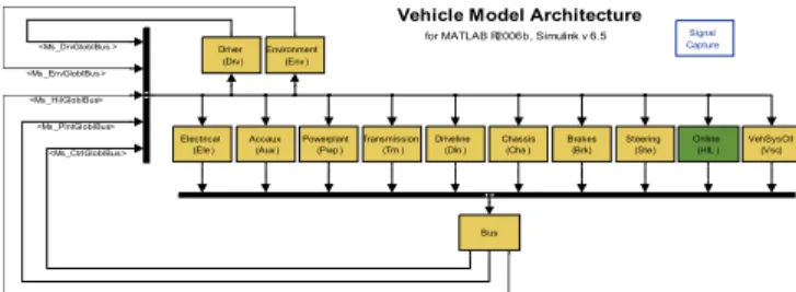
The VMA defines a high-level modular structure for dynamic vehicle modeling with key vehicle subsystems represented as distinct elements. Subsystem connections are specified through well-defined interfaces. As shown in Figure 2, the top-level subsystems are Driver, Environment, Electrical, Auxiliaries, Powerplant, Transmission, Driveline, Chassis, Brakes, Steering, Online HIL, Vehicle System Controller and Bus (Controller and Plant). The NGFCV vehicle system controller is placed in the VSC block in the following Vehicle Model Architecture.
Vehicle Model Architecture
for MATLAB R2006b, Simulink v 6.5 Signal Capture VehSysCtl (Vsc) Transmission (Trn ) Steering (Ste) Powerplant (Pwp ) Online (HIL ) Environment (Env ) Electrical (Ele ) Driver (Drv) Driveline (Dln ) Chassis (Cha ) Bus Brakes (Brk) Accaux (Aux ) <Ms_CtrlGloblBus> <Ms_PlntGloblBus> <Ms_DrvGloblBus > <Ms_EnvGloblBus > <Ms_HilGloblBus>
Figure 2 Vehicle Model Architecture with HIL
For the NGFCV, the powerplant subsystem contains a model of the new generation fuel cell system. The dynamic fuel cell model is capable of accurately simulating new generation fuel cell system performance and critical system dynamics. Four main modules included in the fuel cell plant model are Cathode module, Anode module, Stack module and Electrical module. Although additional proprietary information exists, models parallel to our fuel cell stack model are given in [4-6].
The Electrical subsystem includes a model of the Lithium-Ion battery pack, the HVEC, and the complete electrical bus. The battery is modeled based on an equivalent circuit shown
in Figure 3. The energy captured or delivered from the batteries is accounted for by integrating the power flows into or from the pack and the power losses developed in the battery. Current is integrated to calculate the State of Charge. The internal losses are integrated to calculate the temperature rise within the pack.
Figure 3 Equivalent Circuit Model for the Battery
The Transmission subsystem contains a model of the IPT. It consists of an electric motor, a power electronic assembly with integrated DC/DC converter and a final drive with integrated differential.
A simplified VSC model is used to verify proper integration of all other model components and to give directional guidance for the real VSC debugging work. The load following strategy used in the simple VSC has the following features:
The vehicle control commands the fuel cell system to supply power in direct response to driver wheel power demand.
The vehicle control limits the electrical power allocated to the traction motor according to the power available from the FCS due to FCS dynamic limitations.
Battery state of charge (SOC) is maintained by the vehicle control via a power versus SOC curve. When SOC rises above the high SOC threshold, power is discharged from the battery during traction mode up to the maximum discharge power limit. When SOC drops below the lower SOC threshold, additional FCS power for charging the battery is commanded up to the maximum charge power limit.
Series regenerative brake control is represented. The level of regenerative braking allowed is adjustable. B. Vehicle Controllers
As mentioned earlier, due to the complexity of the FCV, some of the controller modules (i.e. IPT, BCM, FCU shown in Figure 4) were developed by different groups. For the NGFCV, the only modules considered part of the vehicle controls are VSC, EMM and TSC.
CAN bus Instrument Cluster Module (ICM) Brake System Controller (BSC) Integrated Power Train (IPT) Energy Management Module (EMM) Climate System
Controller (CSC) Thermal SystemController (TSC) Fuel Cell controlunit (FCU)
Worldwide Diagnostic System (WDS)
Vehicle System Controller (VSC)
Figure 4 Vehicle Control Modules
The VSC module serves as high-level supervisory controller. It receives CAN and hardware signals such as Ignition Key On/Off, coordinates control actions of
numerous modules, sequence start-up and shutdown, initiate freezing, cold and normal start, and allocate current available from FCU and the hybrid battery to various subsystems in the vehicle. The EMM module serves as a lower level controller (with reference to VSC) responsible for managing the flow of energy on the vehicle high voltage bus, namely distribution of energy on high voltage bus between the heater and the HV battery. The TSC has responsibility for control of three cooling systems (with different levels of operating temperatures) in the NGFCV.
C. Interfacing Plant and Vehicle Controllers
In Figure 2, the overall MIL signal bus architecture is shown. There are five buses: Driver, Bus, Environment Bus, HIL (Hardware-in-the-Loop) Bus, Plant Physical Bus, Control Bus. The HIL bus is a placeholder for future HIL development.
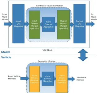
Notice that due to the fact that plant and controller are developed by different teams and with different naming and unit conventions, it is necessary to have "wrappers" to map plant signals to the controller (via "input wrapper"), and to map controller output signals to the plant (via "output wrapper"). Figure 5 shows how the input wrapper layer and output wrapper layer in the controller connect the plant with the controller.
As it is mentioned earlier, input wrapper maps plant signals to the signals that are used by the controller. First, signal from the control bus is selected via a bus selector. The selected signal is then either grouped with other signals to form the CAN bus or the analog input bus, or the digital input bus for the controller.
During the development phase, some input signals to the controller are not generated by the plant model, and similarly some controller output signals are not used by the plant model. For such cases, constants are used for those signals with default values set as nominal values of the associated signals. Similarly controller output signals are collected (within the controller) to form the control bus to feedback to the plant model.
Figure 5 Connecting the plant with the implementation level control algorithms.
The controller structure used in our development is beneficial for rapid simulation or implementation using automatic code generation (a.k.a. autocoding). This enables the developers to build in computer, hardware-in-the-loop and vehicle level applications with minimum effort and errors. Figure 6 summarizes the structure and process of this
approach. The controller model is structured in a way that the portions can be re-used in drag-n-drop fashion for models for different purposes. For example, in order to build the implementation model which is autocoded and run as an application in the vehicle one can use the ‘core control algorithm’ block and with the correct form of ‘Input/Output Driver’ blocks as shown in Figure 6. In [7], development of a hardware-in-the-loop model from the simulation models with a similar approach is discussed for hybrid vehicle development.
Figure 6 Controller Model Interfacing with other models.
III. MIL SYSTEM VERIFICATION AND VALIDATION Two steps of verification and validation studies are performed in this work. First, the MIL model outputs are compared with a simple, yet proven VSC controller output driven by the same inputs. Secondly, the MIL model outputs are compared with dynamometer test data.
Before the verification and validation correlation work, some important variables and their reference values, which are related to the validation process, are studied.
A. Battery Control Strategy and Power Requirement For the majority of existing fuel cell vehicles, battery control strategy utilizes the battery as a source for "fill-in" during transient operation (acceleration and regenerative braking) of the vehicle [8]. When in steady state, battery SOC is expected to be around a desired set point (50%). Hence, for the current study, when steady-state is reached, we expect battery SOC to be at 50%, and no charge/discharge is needed from the battery to support propulsion and/or energy management purposes.
B. Fuel Cell Operating Point
In order to validate the correctness of the MIL model operation, it is very beneficial to check the fuel cell operating point. A fuel cell operating point is a (V, I) point on a fuel cell polarization curve. As it is well known, fuel cell polarization curve has three segments [9]: activation loss segment, ohmic loss segment, and transport loss segment.
Figure 7 Fuel Cell Polarization Curve
The following is a sample polarization curve from fuel cell group for prototype fuel cell stack.
0 0.2 0.4 0.6 0.8 1
0 0.5 1
Normalized V-I and Power Curves
Current (scaled)
V-I curve Power curve
Figure 8 Representative polarization curve (scaled data) C. Real VSC vs. Simple VSC Correlation
To verify the directional correctness of the real VSC, The real VSC and simple VSC are connected closed loop with the plant model respectively. The main characteristic variables from the simulation results are compared.
Some reference values are provided in order to help the correlation study between Real VSC and the Simple VSC.
As it was mentioned earlier, the NGFCV is Ford Explorer based. It is certainly very useful to identify the steady-state propulsion power requirement for such vehicles for a given target speed. In order to calculate the steady state propulsion power requirement, the following assumptions are made:
Drive profile is constant speed; Vehicle has reached steady state;
Driver model is perfect (i.e., no acceleration, deceleration after reaching target speed)
No need for heater operation (cabin heating).
Based on vehicle and test environment data, the steady state power request can be calculated using the propulsion power calculation given in [10].
Notice that there are other direct power requests in the vehicle's high voltage bus, for example, the fuel cell parasitic load (air compressor, HRB (hydrogen recirculation blower)), High Temperature coolant pump (if a high voltage pump is used), and Low Voltage DC/DC converter. Based on real vehicle test data, for a constant speed drive profile of 100 km/h, the parasitic power of the fuel cell and other vehicle accessory power requests are added to the propulsion power request. This is the overall vehicle power request.
To verify the simulation results for a 100 km/h profile, steady state simulation, the following values1 can be
obtained and the polarization curve shown above. Fuel cell power request =0.2027
Fuel cell current =0.2611 (via interpolation) Fuel cell voltage =0.7750 (V=P/I)
1 Current, voltage, power, IPT speed and IPT torque values are scaled
throughout this section.
Figure 9 Pedal position, vehicle speed and acceleration correlation results between real VSC and simple VSC (100 km/h)
Figure 10 Battery SOC, battery voltage and battery current (scaled) correlation results between real VSC and simple VSC (100 km/h)
Figure 11 Fuel cell voltage, current and power (scaled) correlation results between real VSC and simple VSC (100 km/h)
Figure 12 IPT speed, power and torque (scaled) correlation results between real VSC and simple VSC (100 km/h)
From Figure 9, Figure 10, Figure 11 and Figure 12, it can be seen that the Real VSC correlates very well with the Simple VSC for the driving profile considered. The main differences are in SOC traces, which as we mentioned above, can be linked to different energy management strategies, and in traction motor torque (idle situation, in early development stage), which is due to the fact that Real
VSC has minimum torque called "creep torque" when vehicle is in idle. As such, the simple VSC has been modified to represent the real world torque control strategy.
D. MIL Data vs. Vehicle Dynamometer Test Data Comparison
Due to the resource allocation priorities, only one constant speed test was done in the dynamometer with the purpose of comparing vehicle data with the MIL data. At the time of the test, the vehicle had just finished freeze-startup. As such, the fuel cell polarization curve was not up to a level associated with fully warmed up operation [9]. Also, it is realized the driver model (i.e., how the pedal is controlled based on difference between desired and actual vehicle speed) for the MIL behaves differently than the actual driver for the test. Hence the acceleration traces of the vehicle under dynamometer test and in MIL are different. Even with these significant differences, from the comparison shown below, the MIL model produces results that are reasonably consistent with the vehicle.
Again, the drive profile is a 100 km/h, constant speed target with starting speed of zero km/h. From the response curve shown in "Test" (dynamometer test result), it is clear the actual driver on the dynamometer acts differently from the driver model in the MIL.
0 10 20 30 40 50 60 70 80 90 100 110 120 130 140 150
0.6 0.8 1
FCU Voltage Correlation
Time(s) U _F C U (s caled) Mil Test
Figure 13 Comparison of fuel cell voltage (scaled) between MIL and vehicle dynamometer test
Figure 13 shows the fuel cell voltage response curves. Notice that although there are significant differences, key trends are similar: there is a lowered fuel cell voltage (larger fuel cell current according to polarization curve) between 10~25 seconds range. This is due to the high power demand from the driver, which is required to accelerate the vehicle (see Figure 14). Eventually, when the vehicle reaches steady state, the scaled fuel cell bus voltage settles at around 0.775.
0 10 20 30 40 50 60 70 80 90 100 110 120 130 140 150
0 50 100
Vehicle Speed Correlation
Time(s)
V_V
eh(k
ph) Mil
Test
Figure 14 Comparison of vehicle speed between MIL and vehicle dynamometer test
0 10 20 30 40 50 60 70 80 90 100 110 120 130 140 150
0 0.5
1 FCU Current Correlation
Time(s) I_ F C U (s
caled) MilTest
Figure 15 Comparison of fuel cell currents (scaled) between MIL and vehicle dynamometer test
A related variable is fuel cell current.
Figure 15 shows a peak in fuel cell current from 10~25 seconds, consistent with the high power demand from the driver to accelerate the vehicle.
Vehicle bus voltage is the voltage experienced by the HVEC (on vehicle side). Figure 16 shows that except for one stretch after 25 seconds, the vehicle bus voltages for MIL and dynamometer test data are almost the same. The reason for the differences on and after 25 seconds is that during dynamometer test, after acceleration at around 25 seconds, the request for fuel cell current is dropped so the bus voltage is raised (in order to reduce fuel cell current request). On the other hand, there is no such relaxation in the MIL. Similarly, the vehicle bus voltage remains close its steady-state value.
0 10 20 30 40 50 60 70 80 90 100 110 120 130 140 150
0 0.5 1
Vehicle Bus Voltage Correlation
Time(s) U _B us( sc al e d) Mil Test
Figure 16 Comparison of vehicle bus voltages (scaled) between MIL and vehicle dynamometer test
0 10 20 30 40 50 60 70 80 90 100 110 120 130 140 150
0.4 0.6 0.8
Battery Voltage Correlation
Time(s) U_ B att (s ca le d) Mil Test
Figure 17 Comparison of battery bus voltages (scaled) between MIL and vehicle dynamometer test
0 10 20 30 40 50 60 70 80 90 100 110 120 130 140 150
-0.4 -0.2 0 0.2
Battery Current Correlation
Time(s) I_ B att( sc al ed ) Mil Test
Figure 18 Comparison of battery currents (scaled) between MIL and vehicle dynamometer test
Figure 17 and Figure 18 compare battery voltage and current traces between model and test. The battery is used to serve as a buffer for the fuel cell power supply. During the initial tip-in event, the battery voltage drops because the battery is required to supply current to meet motor current demand as the fuel cell current output lags demand. Figure 17 shows the scaled battery voltage eventually settles down at around 0.60 for both MIL and vehicle on the dynamometer.
Figure 18 shows the scaled battery current traces. Battery current increases rapidly during the tip-in event. As discussed above, this is because the fuel cell system response lags motor current demand. The battery makes up the difference. The simulation indicates more battery usage than the actual vehicle. This can at least partly be attributed to differences in driver behavior. Overall battery current levels during the tip-in event show good correlation between simulation and test. As expected, since the battery serves as a power buffer, in steady state for both MIL and dynamometer results vehicle battery current eventually settles to around zero.
Table 1 shows the fuel cell power requirement, fuel cell current, and fuel cell voltage from the reference numbers, simple VSC, MIL model, and the vehicle dynamometer test for the steady-state constant speed drive cycle. The results show good correlation and the simulation model provides a good environment for control development.
Table 1 Summary of Validation Results (scaled data) FC Pwr. Req. FC Current Volt. FC Reference Values 0.2027 0.2611 0.775 Simple VSC 0.2071 0.2668 0.774 MIL Model 0.2071 0.2668 0.774 Dynamometer Test 0.2231 0.2861 0.78
Remark: The last column shows that the real fuel cell
polarization curve at the test temperature is slightly different from the polarization shown in Figure 9.
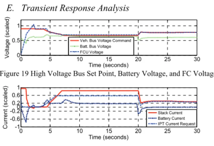
E. Transient Response Analysis
0 5 10 15 20 25 30 0 0.5 1 Time (seconds) Volt age ( sc al ed)
Veh. Bus Voltage Command Batt. Bus Voltage FCU Voltage
Figure 19 High Voltage Bus Set Point, Battery Voltage, and FC Voltage
0 5 10 15 20 25 30 -1 -0.6 -0.2 0.2 0.6 1 0 Time (seconds) C u rren t (s ca le d) Stack Current Battery Current IPT Current Request
Figure 20 Stack Current, Battery Current, and Motor Current Request In Figure 19 and Figure 20, the transient responses of the MIL model for a full pedal acceleration up to a constant speed of 100 km/h are shown. Figure 19 shows the bus voltage set point trace and the fuel cell voltage trace for the acceleration event. The bus voltage set point trace represents the target voltage commanded to the HVEC. The voltage set point initially decreases in response to high driver wheel torque demand. As the driver reduces accelerator pedal when the vehicle reaches 100 km/h at around 20 second, the set point voltage rises. The fuel cell voltage tracks the set point voltage very closely, indicating that the HVEC control in the simulation is behaving properly.
In Figure 20, the fuel cell current, battery current and motor current request is shown. Motor current and stack current both increase rapidly during the driver tip-in event. The fuel cell cannot respond fast enough to the motor current demand; therefore a significant amount of battery current is used to provide the remainder of the current needed by the motor to produce the driver demanded torque. When the vehicle reaches a speed of 100 km/h, the driver tips out and the motor current demand drops rapidly. The
driver applies a small amount of brake pedal to control vehicle speed, which causes the motor current demand to go negative, indicating a regenerative braking event. Some current flows to the battery as indicated by the negative battery current spike is also noticed. Stack current drops to a very low level during the tip out event. It then recovers to a small steady state level as vehicle speed stabilizes. Overall the behavior of the stack, battery and motor current indicates that the simulation is working as expected.
IV. CONCLUSION AND DISCUSSION
In this paper the development of a MIL system for NGFCV is described. Verification and validation methodologies and results are presented. From comparison between real and simple VSC controls in desktop simulation, and from comparison between dynamometer test data of the NGFCV, and the real VSC control in the MIL, it is clear that the MIL system can be used with fidelity to simulate real time controls, and to assist development of new vehicle control strategies before hardware becomes available.
A rapid model building approach, which is suitable for model-based controller design process, was also discussed. The approach minimizes the model development times for different platforms while minimizing the possibilities for modeling and implementation errors.
ACKNOWLEDGEMENTS
The authors would like to thank Mark Jennings, Ray Spiteri, Alex Zaremba, John Blankenship, Judy Che, Ramzi Chraim, Fangyi Zhao, Fangjun Jiang, Hasdi Hashim, and Craig Mathie for their help and contributions.
REFERENCES
[1] W. Yang, B. Bates, N. Fletcher, and R. Pow, “Control challenges and methodologies in fuel cell vehicle development,” SAE Paper 98C054, 1998.
[2] R. C. Hill, J. Lockwood, and Y. Li, “Diagnostics Design Process for Developmental Vehicles,” SAE Paper 2010-01-0247, 2010.
[3] C. Belton, et al, “A Vehicle Model Architecture for Vehicle System Control Design,” SAE Paper 2003-01-0092, 2003.
[4] J. T. Pukrushpan, H. Peng, and A. G. Stefanopoulou, “Control-oriented modeling and analysis for automotive fuel cell systems,”
Journal of dynamic systems, measurement, and control, vol. 126, p.
14, 2004.
[5] J. T. Pukrushpan, A. G. Stefanopoulou, and H. Peng, Control of fuel
cell power systems: principles, modeling, analysis, and feedback design. Springer Verlag, 2004.
[6] L. Guzzella and A. Sciarretta, Vehicle propulsion systems:
introduction to modeling and optimization. Springer, 2007.
[7] Y. Zhao, Z. Yan, J. Blankenship, and M. Cakmakci, “Development of a Hardware-In-The-Loop System for a Hybrid Powertrain Vehicle Control,” presented at the Global Powertrain Congress, Chicago, 2008.
[8] T. Hunter, R. Spiteri, Method and System for Controlling Power Distribution in a Hybrid Fuel Cell Vehicle, US Patent 6792341, Sept. 14, 2004.
[9] A. Dicks and J. Larminie, Fuel cell systems explained. John Wiley & Sons, 2000.
[10] T. D. Gillespie, Fundamentals of Vehicle Dynamics. SAE International, 1992.
2467
View publication stats View publication stats