High-sensitivity noncontact atomic force microscope
Õ
scanning tunneling
microscope
„
nc AFM
Õ
STM
…
operating at subangstrom oscillation
amplitudes for atomic resolution imaging and force spectroscopy
A. Oral,a),b)R. A. Grimble, H. O¨ . O¨zer,b)and J. B. Pethica
Department of Materials, University of Oxford, Parks Road, Oxford OX1 3PH, United Kingdom 共Received 27 August 2002; accepted 27 May 2003兲
We describe a new, highly sensitive noncontact atomic force microscope/scanning tunneling microscope共STM兲 operating in ultrahigh vacuum 共UHV兲 with subangstrom oscillation amplitudes for atomic resolution imaging and force–distance spectroscopy. A novel fiber interferometer with ⬃4⫻10⫺4Å/
冑
Hz noise level is employed to detect cantilever displacements. Subangstromoscillation amplitude is applied to the lever at a frequency well below the resonance and changes in the oscillation amplitude due to tip–sample force interactions are measured with a lock-in amplifier. Quantitative force gradient images can be obtained simultaneously with the STM topography. Employment of subangstrom oscillation amplitudes lets us perform force–distance measurements, which reveal very short-range force interactions, consistent with the theory. Performance of the microscope is demonstrated with quantitative atomic resolution images of Si共111兲共7⫻7兲 and force– distance curves showing short interaction range, all obtained with ⬍0.25 Å lever oscillation amplitude. Our technique is not limited to UHV only and operation under liquids and air is feasible. © 2003 American Institute of Physics. 关DOI: 10.1063/1.1593786兴
I. INTRODUCTION
At its invention, the atomic force microscope 共AFM兲 共Ref. 1兲 was intended to be an analogue of the scanning tunneling microscope共STM兲, using the forces rather than the tunnel current between tip and surface atoms to generate an image. In principle, this should also give atomic resolution because short-range bonds such as covalent, have, like tunnel current, an exponential dependence on distance.2,3The rapid-ity of exponential decay is generally accepted to be the rea-son for the high resolution. However, the actual development and wide applicability of AFM has mostly been at poorer resolution than atomic, mainly because of the extreme sensi-tivity required to resolve single bonds and the instability of soft, sensitive levers against high force gradients of short-range interactions. Atomic resolution AFM has been achieved using resonant cantilevers with large,⬃100 Å, os-cillation amplitudes in UHV.4 – 6 This technique is also used to deduce the force interactions between tip and sample, but large oscillation amplitudes employed are vastly greater than the interaction range and the interaction has to be deduced by using a deconvolution in which assumptions such as single valuedness, no loss, etc., have to be made.7 Durig et al.8 measured the short range interactions using an Ir sample for the first time, but this work did not involve any imaging. Other attempts9,10 for direct observations of the form of the bonding interaction have so far shown unexpectedly large length scales, which are incompatible with a true strong atomic bond.11
In this article, we describe a new combined noncontact AFM 共nc-AFM兲 and STM that can operate at subangstrom oscillation amplitudes using stiff (k⬃100 N/m) cantilevers below resonance, which would allow quantitative atomic resolution imaging and force–distance spectroscopy. Use of sub-Å lever oscillation amplitudes simplifies the data analy-sis and allows direct determination of the interaction poten-tial without the need for deconvolution of data from reso-nance shifts.7,12,13 Quantitative values of the bond stiffness values during imaging of Si共111兲共7⫻7兲 are thereby obtained.14 Furthermore, our technique operates in the liquids15 without loss of any sensitivity and has potential to achieve atomic resolution in liquids and in air.
II. INSTRUMENTATION A. UHV system
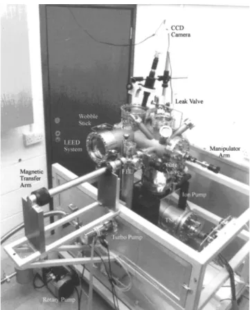
The microscope is installed in a small, custom-designed ultra-high-vacuum 共UHV兲 chamber, as shown in Fig. 1, which is equipped with a low-energy electron diffraction 共LEED兲/Auger16 system for sample analysis, argon
sputter-ing gun and a home made electron beam heater for sample/ lever preparation. The system volume and surface area have been kept very small to achieve a low base pressure in the system. The main chamber is pumped with a combination pump, which is composed of a 300 l/s共Ref. 17兲 triode pump and a titanium sublimation pump. A small, 70 l/s turbomo-lecular pump18 backed with a double stage rotary pump is used to evacuate the fast entry lock for lever/sample transfer. An 8 in. travel linear-rotary motion feedthrough is employed as sample/lever manipulator. After baking the system out at 165 °C, a base pressure of ⬃7⫻10⫺11mbar is routinely
a兲Author to whom correspondence should be addressed; electronic mail: [email protected]
b兲Present address: Department of Physics, Bilkent University, 06533 Ankara, Turkey.
3656
achieved. Atomically clean Si共111兲共7⫻7兲 is prepared in situ by standard methods finally flashing the sample to 1000 °C. B. NC-AFMÕSTM
Our microscope is built on a special 8-in.-diam conflate UHV flange as shown in the Fig. 2. The design allows us to exchange levers and samples without breaking the vacuum through the load lock. Up to four samples/levers can be stored in a carousel attached to the microscope, which also acts as sample holder for LEED/Auger analysis. For vibra-tion isolavibra-tion, microscope base is suspended from four posts by using stainless steel springs and Sm–Co magnet–copper sheet pairs are used for eddy current damping. This configu-ration has a natural frequency of ⬃2 Hz and is sufficient to eliminate the external vibrations in our laboratory, which is located at the first floor. During the lever/sample transfer, the microscope base and the sample slider are locked to the four posts by a special mechanism actuated with a linear motion
into UHV by a home-made fiber feedthrough.21A small hole is drilled into a 1.33 in. CF blank flange, the fiber’s plastic cladding is stripped before the fiber is fed through the hole and glued using Torr Seal.22
The cantilever is held fixed and the sample is scanned by using an EBL No. 2 piezotube23in our microscope design as shown in Fig. 2. A piezoplate glued at the cantilever mount-ing block is used to vibrate the cantilevers. The cantilever displacements are measured with a novel all-fiber interfer-ometer positioned accurately at the back of the cantilever with a piezodriven five-axis stick–slip slider. The scanner piezotube is mounted on another shear piezodriven stick–slip slider for coarse approach. Small, 1-mm-diam SiN balls are glued to the shear piezostacks24fixed to the microscope base, which slide on polished sapphire plates attached to the sample slider block. Sample slider can move in z and y di-rections and rotate around the x axis. Small Sm–Co magnets and nickel sheets are used to pull the sample slider block towards the AFM base to increase the stiffness of the system. The bias voltage is applied to the cantilever and the tunnel-ing current is measured from the sample with an in vacuum operational amplifier25and a 100 M⍀ feedback resistor, both placed just at the back of the scan tube. A stainless steel shield is mounted on the scan tube to minimize the capaci-tive coupling of high voltage scan signals to the tunnel cur-rent.
1. Fiber slider
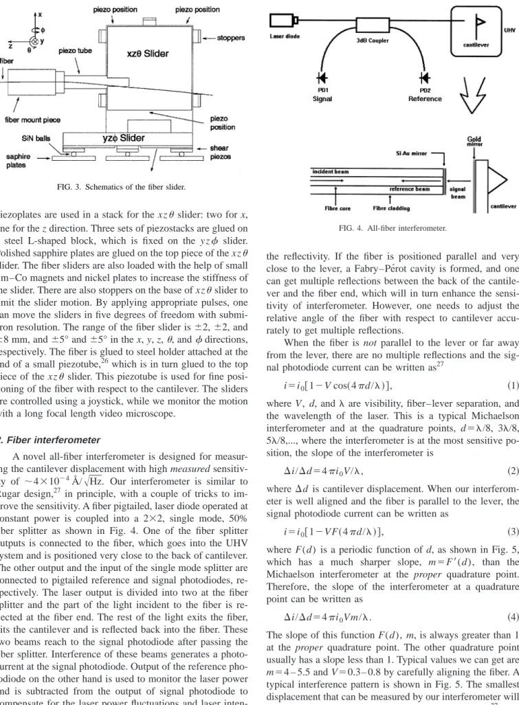
We realized a high-precision and reliable five-axis posi-tioner is required for the desired sensitivity levels of our microscope. The fiber is positioned at the back of cantilever by using a fiber slider, which has five degrees of freedom; three directions, x, y, z and two rotations,and. The fiber slider design, which is shown in Fig. 3, is similar to sample slider, but smaller in dimensions. Two piezodriven stick–slip sliders (y z and xz sliders兲, which can move in a plane and rotate around the axis normal to the plane are mounted on top of each other to form the fiber slider, which can move in five degrees of freedom. For the y z slider, which can move parallel to the microscope base and rotate, two shear plates are glued on top of each other with orthogonal polar-ization direction and then to the slider block. There are three sets of shear plates like this in the slider and 1-mm-diam SiN balls are glued to the piezoplates, which slide on polished sapphire plates fixed at the nc-AFM base. Since it is always more difficult to move against the gravity, three shear
FIG. 1. Picture of the UHV system.
piezoplates are used in a stack for the xz slider: two for x, one for the z direction. Three sets of piezostacks are glued on a steel L-shaped block, which is fixed on the y z slider. Polished sapphire plates are glued on the top piece of the xz slider. The fiber sliders are also loaded with the help of small Sm–Co magnets and nickel plates to increase the stiffness of the slider. There are also stoppers on the base of xz slider to limit the slider motion. By applying appropriate pulses, one can move the sliders in five degrees of freedom with submi-cron resolution. The range of the fiber slider is⫾2, ⫾2, and ⫾8 mm, and ⫾5° and ⫾5° in the x, y, z,, anddirections, respectively. The fiber is glued to steel holder attached at the end of a small piezotube,26which is in turn glued to the top piece of the xz slider. This piezotube is used for fine posi-tioning of the fiber with respect to the cantilever. The sliders are controlled using a joystick, while we monitor the motion with a long focal length video microscope.
2. Fiber interferometer
A novel all-fiber interferometer is designed for measur-ing the cantilever displacement with high measured sensitiv-ity of ⬃4⫻10⫺4Å/
冑
Hz. Our interferometer is similar to Rugar design,27 in principle, with a couple of tricks to im-prove the sensitivity. A fiber pigtailed, laser diode operated at constant power is coupled into a 2⫻2, single mode, 50% fiber splitter as shown in Fig. 4. One of the fiber splitter outputs is connected to the fiber, which goes into the UHV system and is positioned very close to the back of cantilever. The other output and the input of the single mode splitter are connected to pigtailed reference and signal photodiodes, re-spectively. The laser output is divided into two at the fiber splitter and the part of the light incident to the fiber is re-flected at the fiber end. The rest of the light exits the fiber, hits the cantilever and is reflected back into the fiber. These two beams reach to the signal photodiode after passing the fiber splitter. Interference of these beams generates a photo-current at the signal photodiode. Output of the reference pho-todiode on the other hand is used to monitor the laser power and is subtracted from the output of signal photodiode to compensate for the laser power fluctuations and laser inten-sity noise. The end of the fiber is first cleaved with a preci-sion fiber cleaver and then coated with Si and Au to enhancethe reflectivity. If the fiber is positioned parallel and very close to the lever, a Fabry–Pe´rot cavity is formed, and one can get multiple reflections between the back of the cantile-ver and the fiber end, which will in turn enhance the sensi-tivity of interferometer. However, one needs to adjust the relative angle of the fiber with respect to cantilever accu-rately to get multiple reflections.
When the fiber is not parallel to the lever or far away from the lever, there are no multiple reflections and the sig-nal photodiode current can be written as27
i⫽i0关1⫺V cos共4d/兲兴, 共1兲
where V, d, and are visibility, fiber–lever separation, and the wavelength of the laser. This is a typical Michaelson interferometer and at the quadrature points, d⫽/8, 3/8, 5/8,..., where the interferometer is at the most sensitive po-sition, the slope of the interferometer is
⌬i/⌬d⫽4i0V/, 共2兲
where⌬d is cantilever displacement. When our interferom-eter is well aligned and the fiber is parallel to the lever, the signal photodiode current can be written as
i⫽i0关1⫺VF共4d/兲兴, 共3兲
where F(d) is a periodic function of d, as shown in Fig. 5, which has a much sharper slope, m⫽F
⬘
(d), than the Michaelson interferometer at the proper quadrature point. Therefore, the slope of the interferometer at a quadrature point can be written as⌬i/⌬d⫽4i0Vm/. 共4兲
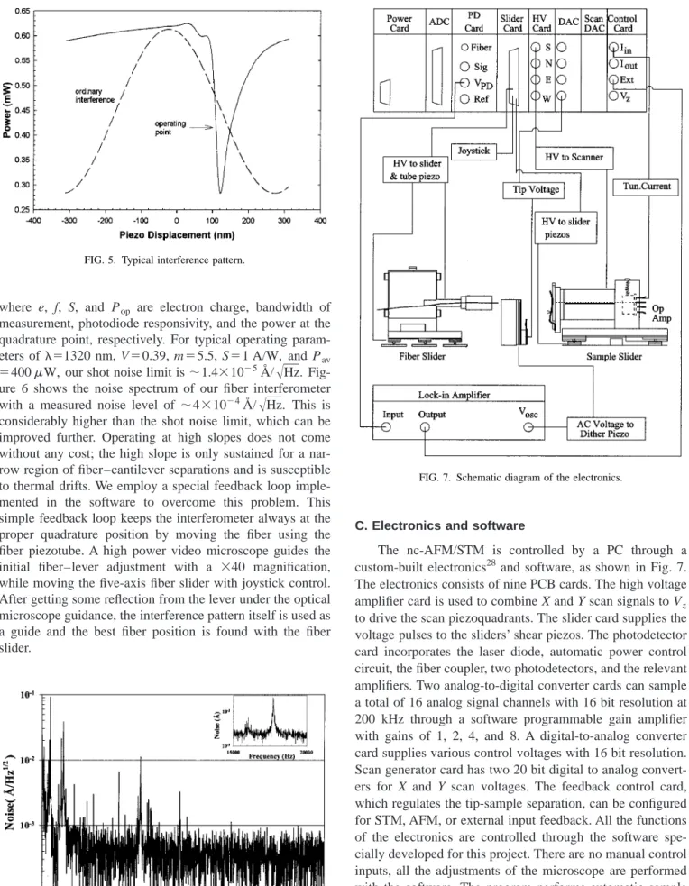
The slope of this function F(d), m, is always greater than 1 at the proper quadrature point. The other quadrature point usually has a slope less than 1. Typical values we can get are m⫽4 – 5.5 and V⫽0.3– 0.8 by carefully aligning the fiber. A typical interference pattern is shown in Fig. 5. The smallest displacement that can be measured by our interferometer will be limited by the shot noise, which can be written as27
dshot⫽共/2Vm兲冑共e f /2SPop兲, 共5兲
FIG. 3. Schematics of the fiber slider.
where e, f, S, and Pop are electron charge, bandwidth of
measurement, photodiode responsivity, and the power at the quadrature point, respectively. For typical operating param-eters of ⫽1320 nm, V⫽0.39, m⫽5.5, S⫽1 A/W, and Pav
⫽400W, our shot noise limit is⬃1.4⫻10⫺5Å/
冑
Hz. Fig-ure 6 shows the noise spectrum of our fiber interferometer with a measured noise level of ⬃4⫻10⫺4Å/冑
Hz. This is considerably higher than the shot noise limit, which can be improved further. Operating at high slopes does not come without any cost; the high slope is only sustained for a nar-row region of fiber–cantilever separations and is susceptible to thermal drifts. We employ a special feedback loop imple-mented in the software to overcome this problem. This simple feedback loop keeps the interferometer always at the proper quadrature position by moving the fiber using the fiber piezotube. A high power video microscope guides the initial fiber–lever adjustment with a ⫻40 magnification, while moving the five-axis fiber slider with joystick control. After getting some reflection from the lever under the optical microscope guidance, the interference pattern itself is used as a guide and the best fiber position is found with the fiber slider.C. Electronics and software
The nc-AFM/STM is controlled by a PC through a custom-built electronics28 and software, as shown in Fig. 7. The electronics consists of nine PCB cards. The high voltage amplifier card is used to combine X and Y scan signals to Vz
to drive the scan piezoquadrants. The slider card supplies the voltage pulses to the sliders’ shear piezos. The photodetector card incorporates the laser diode, automatic power control circuit, the fiber coupler, two photodetectors, and the relevant amplifiers. Two analog-to-digital converter cards can sample a total of 16 analog signal channels with 16 bit resolution at 200 kHz through a software programmable gain amplifier with gains of 1, 2, 4, and 8. A digital-to-analog converter card supplies various control voltages with 16 bit resolution. Scan generator card has two 20 bit digital to analog convert-ers for X and Y scan voltages. The feedback control card, which regulates the tip-sample separation, can be configured for STM, AFM, or external input feedback. All the functions of the electronics are controlled through the software spe-cially developed for this project. There are no manual control inputs, all the adjustments of the microscope are performed with the software. The program performs automatic sample approach, image acquisition, force–distance curve, interfer-ence pattern measurements, quadrature locking for staying at highest sensitivity point, image display, and various postac-quisition image manipulations.
FIG. 5. Typical interference pattern.
FIG. 6. Noise spectrum of the fiber interferometer obtained with a tungsten cantilever in UHV.
D. Operation of the microscope
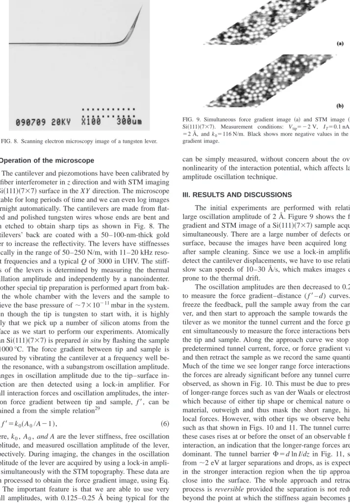
The cantilever and piezomotions have been calibrated by the fiber interferometer in z direction and with STM imaging of Si共111兲共7⫻7兲 surface in the XY direction. The microscope is stable for long periods of time and we can even log images overnight automatically. The cantilevers are made from flat-tened and polished tungsten wires whose ends are bent and then etched to obtain sharp tips as shown in Fig. 8. The cantilevers’ back are coated with a 50–100-nm-thick gold layer to increase the reflectivity. The levers have stiffnesses typically in the range of 50–250 N/m, with 11–20 kHz reso-nant frequencies and a typical Q of 3000 in UHV. The stiff-ness of the levers is determined by measuring the thermal oscillation amplitude and independently by a nanoindenter. No other special tip preparation is performed apart from bak-ing the whole chamber with the levers and the sample to achieve the base pressure of⬃7⫻10⫺11mbar in the system. Even though the tip is tungsten to start with, it is highly likely that we pick up a number of silicon atoms from the surface as we start to perform our experiments. Atomically clean Si共111兲共7⫻7兲 is prepared in situ by flashing the sample to 1000 °C. The force gradient between tip and sample is measured by vibrating the cantilever at a frequency well be-low the resonance, with a subangstrom oscillation amplitude. Changes in oscillation amplitude due to the tip–surface in-teraction are then detected using a lock-in amplifier. For small interaction forces and oscillation amplitudes, the inter-action force gradient between tip and sample, f
⬘
, can be obtained a from the simple relation29f
⬘
⫽k0共A0/A⫺1兲, 共6兲where, k0, A0, and A are the lever stiffness, free oscillation amplitude, and measured oscillation amplitude of the lever, respectively. During imaging, the changes in the oscillation amplitude of the lever are acquired by using a lock-in ampli-fier simultaneously with the STM topography. These data are then processed to obtain the force gradient image, using Eq. 共6兲. The important feature is that we are able to use very small amplitudes, with 0.125–0.25 Å being typical for the data in this paper. Therefore, even strongly varying forces
can be simply measured, without concern about the overall nonlinearity of the interaction potential, which affects larger amplitude oscillation technique.
III. RESULTS AND DISCUSSIONS
The initial experiments are performed with relatively large oscillation amplitude of 2 Å. Figure 9 shows the force gradient and STM image of a Si共111兲共7⫻7兲 sample acquired simultaneously. There are a large number of defects on the surface, because the images have been acquired long time after sample cleaning. Since we use a lock-in amplifier to detect the cantilever displacements, we have to use relatively slow scan speeds of 10–30 Å/s, which makes images quite prone to the thermal drift.
The oscillation amplitudes are then decreased to 0.25 Å to measure the force gradient–distance ( f
⬘
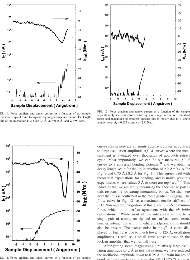
– d) curves. We freeze the feedback, pull the sample away from the cantile-ver, and then start to approach the sample towards the can-tilever as we monitor the tunnel current and the force gradi-ent simultaneously to measure the force interactions between the tip and sample. Along the approach curve we stop at a predetermined tunnel current, force, or force gradient value, and then retract the sample as we record the same quantities. Much of the time we see longer range force interactions and the forces are already significant before any tunnel current is observed, as shown in Fig. 10. This must be due to presence of longer-range forces such as van der Waals or electrostatic, which because of either tip shape or chemical nature of tip material, outweigh and thus mask the short range, highly local forces. However, with other tips we observe behavior such as that shown in Figs. 10 and 11. The tunnel current in these cases rises at or before the onset of an observable force interaction, an indication that the longer-range forces are not dominant. The tunnel barrier ⌽⫽d ln I/dz in Fig. 11, starts from⬃2 eV at larger separations and drops, as is expected30 in the stronger interaction region when the tip approaches close into the surface. The whole approach and retraction process is reversible provided the separation is not reduced beyond the point at which the stiffness again becomes posi-tive共the point of inflection of the binding energy curve兲. TheFIG. 8. Scanning electron microscopy image of a tungsten lever.
FIG. 9. Simultaneous force gradient image 共a兲 and STM image 共b兲 of Si共111兲共7⫻7兲. Measurement conditions: Vtip⫽⫺2 V, IT⫽0.1 nA, A0
⫽2 Å, and k0⫽116 N/m. Black shows more negative values in the force
curves shown here are all single approach curves in contrast to large oscillation amplitude ⌬ f – d curves where the mea-surement is averaged over thousands of approach–retract cycle. Most importantly, we can fit our measured f
⬘
– d curves to a universal bonding potential31 and we obtain a decay length scale for the tip interaction of 2.2 Å⫾0.4 Å for Fig. 9 and 0.75 Å⫾0.2 Å for Fig. 10. This agrees well with theoretical expectations for bonding, and is unlike previous experiments where values 3 Å or more are reported.9,10This indicates that we are really measuring the short-range poten-tials responsible for strong interatomic bonds. We shall see next that this is confirmed in the force gradient imaging. The f⬘
– d curve in Fig. 12 has a maximum tensile stiffness of ⬃13 N/m and the integration of this gives ⬃3 nN maximum force, which is in perfect agreement with the ab initio calculations.11 While most of the interaction is due to a single pair of atoms, on tip and on surface, some extra, smaller, interactions with immediately adjacent atoms should also be present. The excess noise in the f⬘
– d curve dis-played in Fig. 12 is due to much lower, 0.125 Å, oscillation amplitudes as well as a small time constant used in the lock-in amplifier that we normally use.After getting some images using a relatively large oscil-lation amplitude of 2 Å to test the system, we have reduced the oscillation amplitude down to 0.25 Å to obtain images of bond stiffness variations across the Si共111兲共7⫻7兲 surface. Figure 13 shows force gradient and STM topography images obtained simultaneously on a Si共111兲共7⫻7兲 sample. A crucial FIG. 10. Force gradient and tunnel current as a function of tip–sample
separation. Typical result for tips having longer range interaction. The length scale of the interaction is 2.2 Å⫾0.4 Å. A0⫽0.25 Å, and k0⫽90 N/m.
FIG. 11. Force gradient and tunnel current as a function of tip–sample separation. Typical result for tips having short-range interaction. The length scale of the interaction is 0.75 Å⫾0.2 Å found from the fit 共thin line兲. A0
⫽0.25 Å and k0⫽250 N/m.
FIG. 12. Force gradient and tunnel current as a function of tip–sample separation. Typical result for tips having short-range interaction. The short range and magnitude of gradient indicate this is mostly due to a single atomic bond. A0⫽0.125 Å and k0⫽250 N/m.
point is that we were only able to obtain atomic resolution in the force images, such as shown in Fig. 9, when the tips also gave short-range interactions such as that shown in Figs. 11 and 12. This clearly supports the traditional supposition that atomic resolution in AFM requires a rapid exponential inter-action, hence sharp tips. Bond stiffness images such as Fig. 13 give direct quantitative data. First of all, it should be noted that STM topography and force gradient images, al-though broadly similar, do not show exactly the same fea-tures. For example, the areas circled in Fig. 13 show that the missing adatoms in the STM image give a different contrast in AFM image, perhaps due to an adsorbate on the surface. We find that the corrugation from adatom to adatom via cor-ner hole 共line A兲 and from adatom to adatom via restatom 共line B兲 are 12 and 4.5 N/m, respectively. The black shows higher attractive stiffness in the force gradient images, and therefore, the corner holes and restatoms actually have higher attractive stiffness than the adatoms. The force gradi-ent contrast is also seen to increase with decreasing separa-tion at higher tunnel currents. Similar behavior has also been observed on the Si共100兲共2⫻1兲32surface in our recent experi-ments.
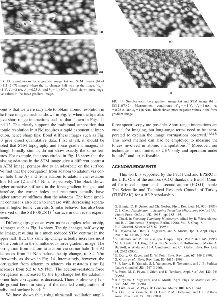
Differing tips give an even more complex relationship, as images such as Fig. 14 show. The tip changes half way up the image, resulting in a much reduced STM contrast in the upper half. But, this same tip change actually increases most of the contrast in the simultaneous force gradient image. The corrugation from adatom to adatom via corner hole共line A兲 decreases from 11 N/m before the tip change, to 8.4 N/m afterwards, as shown in Fig. 14. Interestingly, however, the corrugation from adatom to adatom via restatom 共line B兲 increases from 5.2 to 6.9 N/m. The adatom–restatom force corrugation is increased by the tip change but the adatom– corner hole corrugation is decreased. There is obviously fer-tile ground here for study of the detailed configuration of individual surface bonds.14
We have shown that, using ultrasmall oscillation ampli-tudes, atom-resolved quantitative AFM imaging, and direct
force spectroscopy are possible. Short-range interactions are crucial for imaging, but long-range terms need to be incor-porated to explain the image corrugations observed.14,32,33 This novel method can also be employed to measure the forces involved in atomic manipulations.34 Moreover, our technique is not limited to UHV only and operation under liquids15 and air is feasible.
ACKNOWLEDGMENTS
This work is supported by the Paul Fund and EPSRC in the U.K. One of the authors共A.O.兲 thanks the British Coun-cil for travel support and a second author 共H.O¨.O¨兲 thanks The Scientific and Technical Research Council of Turkey 共TU¨BI˙TAK兲 for a BDP scholarship.
1G. Binnig, C. F. Quate, and Ch. Gerber, Phys. Rev. Lett. 56, 930共1986兲. 2C. J. Chen, Introduction to Scanning Tunneling Microscopy共Oxford
Uni-versity Press, Oxford, UK, 1993兲, pp. 185–193.
3
S. Ciraci, in Scanning Tunneling Microscopy, edited by R. Wiesendanger and H.-J. Guntherodt共Springer, Berlin, 1996兲, Vol. 3, Chap. 8.
4F. J. Giessibl, Science 267, 69共1995兲.
5H. Ueyama, M. Ohta, Y. Sugawara, and S. Morita, Jpn. J. Appl. Phys.,
Part 2 34, L1086共1995兲.
6
S. Kitamura and M. Iwatsuki, Jpn. J. Appl. Phys., Part 2 34, L145共1995兲.
7M. A. Lantz, H. J. Hug, P. J. A. van Schendel, R. Hoffmann, S. Martin, A.
Baratoff, A. Abdurixit, H.-J. Gu¨ntherodt, and Ch. Gerber, Phys. Rev. Lett.
84, 2642共2000兲.
8
U. Du¨rig, O. Zu¨ger, and D. W. Pohl, Phys. Rev. Lett. 65, 349共1990兲.
9G. Cross et al., Phys. Rev. Lett. 80, 4685共1998兲.
10S. P. Jarvis, H. Yamada, S.-I. Yamamoto, H. Tokumoto, and J. B. Pethica,
Nature共London兲 384, 247 共1996兲.
11R. Perez, M. C. Payne, I. Stich, and K. Terakura, Appl. Surf. Sci. 123, 249
共1998兲.
12H. Ueyama, Y. Sugawara, and S. Morita, Appl. Phys. A: Mater. Sci.
Pro-cess. A66, 295共1998兲.
13R. Lu¨thi et al., Z. Phys. B: Condens. Matter 100, 165共1996兲. 14
A. Oral, R. A. Grimble, H. O¨ . O¨zer, P. M. Hoffmann, and J. B. Pethica, Appl. Phys. Lett. 79, 1915共2001兲.
15S. Jeffery, Ph.D. thesis, Oxford University共2001兲.
FIG. 13. Simultaneous force gradient image 共a兲 and STM images 共b兲 of Si共111兲共7⫻7兲 sample where the tip changes half way up the image. Vtip⫽
⫺1 V, IT⫽2 nA, A0⫽0.25 Å, and k0⫽116 N/m. Black shows more
nega-tive values in the force gradient image.
FIG. 14. Simultaneous force gradient image 共a兲 and STM image 共b兲 of Si共111兲共7⫻7兲. Measurement conditions: Vtip⫽⫺1 V, IT⫽1 nA, A0
⫽0.25 Å, and k0⫽116 N/m. Black shows more negative values in the force