A new dominance rule to minimize total weighted tardiness on a single machine

(1)

/ y- ‘.Й; T S ' У 4 5 · I 9 3 S ÜC, и m г л ra R î 3 ? a ѳ ? і і ш н е т і ш r a i f f i i s i s T O f IM Г У If !3nr. m

Ш і Ш OF ІОІШСі

iahmaî Ш ш т W s m

(2)

A NEW DOMINANCE RULE TO MINIMIZE TOTAL

WEIGHTED TARDINESS ON A SINGLE MACHINE

A THESIS

SUBM ITTED TO THE DEPARTMENT OF INDUSTRIAL ENGINEERING

AND THE INSTITUTE OF ENGINEERING AND SCIENCE OF BILKENT UNIVERSITY

IN PARTIAL FULFILLMENT OF THE REQUIREMENTS FOR THE DEGREE OF

MASTER OF SCIENCE

By

jJâA/ıeiÂ...&a^c^·^... ,

Mehmet Bayram Yıldırım

July, 1996

(3)

r s

< 5 ? . S'

(4)

11

I certify that I have read this thesis and that in my opinion it is fully adequate, in scope and in quality, as a thesis for the degree of Master of Science.

Assist. Prof. M. Selim Aktiirk (Advisor)

I certify that I have read this thesis and that in my opinion it is fully adequate, in scope and in quality, as a thesis for the degree ofllylaster of Science.

I certify that I have read this thesis and that in my opinion it is fully adequate, in scope and in quality, as a thesis for the degree of Master of Science.

r:·'

Assist. Prof. Serpil Sayın

Approved for the Institute of Engineering and Sciences:

Prof. Mehmet Elaray

(5)

ABSTRACT

A NEW DOMINANCE RULE TO MINIMIZE TOTAL

WEIGHTED TARDINESS ON A SINGLE MACHINE

Mehmet Bayram Yıldırım

M.S. in Industrial Engineering

Supervisor: Assist. Prof. M. Selim Aktiirk

July, 1996

We present a new dominance rule for the single machine total weighted tardiness problem with job dependent penalties. The proposed dominance rule provides a sufficient condition for local optimality, i.e. if any sequence violates the dominance rule, switching a violating job either lowers the total weighted tardiness or leaves it unchanged. We introduce an algorithm based on the dominance rule, which is compared to a number of competing heuristics for a set of randomly generated problems. Our computational results over •30000 problems indicate that the proposed algorithm dominates the competing heuristics in all runs. Furthermore, the new dominance rules can be used in reducing the number of alternatives for finding the optimal solution in complete enumeration techniques. We show that the proposed dominance rule increases the number of global dominance relationships generated by the Emmons’ Rule which is used heavily in literature to restrict the search space. We also show that having a better upper bound value usually improves the lower bound value which is obtained from the linear lower bound.

Key words: Dominance Rules, Heuristics, Lower Bounds, Single Machine

Scheduling, Upper Bounds.

(6)

ÖZET

ТЕК MAKİNADA TOPLAM AĞIRLIKLI GECİKME

PROBLEMİ İÇİN YENİ BASKINLIK ÖZELLİKLERİ

Mehmet Bayram Yıldırım

Endüstri Mühendisliği Bölümü Yüksek Lisans

Tez Yöneticisi: Yard. Doç. Dr. M. Selim Aktürk

Temmuz, 1996

Bu çalışmada, tek makinada toplam ağırlıklı gecikmeyi en aza indirgeme problemi için yeni baskınlık özellikleri olduğunu göstererek, bu baskınlık özelliklerini kullanan bir algoritma geliştirdik. Bu algoritma yerel en aza indirgemeyi garanti etmekte yani komşu işlerin yerlerinin değiştirilmesi ile daha iyi bir amaç fonksiyonu değerinin bulunamayacağını göstermektedir. Bu baskınlık kuramına göre yapılan değişiklikler ya toplam ağırlıklı gecikmeyi azaltm akta ya da aynı bırakmaktadır.

Literatürde tam sonucu bulmak için kullanılan Emmons kurallarının oluşturduğu genel baskınlık özelliği sayısından daha fazla genel baskınlık özelliği bulundu ve bu baskınlık özellikleri hem alt sınır hem de üst sınır hesaplamalarında kullanıldı. Üst sınırlarda test edilen bütün problemler için iyileştirme sağlanırken, alt sınırlamalarda genelde bir iyileştirme sağlandı.

Anahtar sözcükler: Tek Makinada Çizelgeleme, Toplam Ağırlıklı Gecikmeyi

En Azlama, Baskınlık Kuralları, Alttan Sınırlama, Üstten Sınırlama, Sezgisel Algoritmalar.

(7)

(8)

ACKNOWLEDGEMENT

I am indebted to Assist. Prof. Selim Aktiirk for his invaluable guidance,

encouragement and above all, for the enthusiasm which he inspired on me during this study.

I am also indebted to Assist. Prof. Cemal Akyel and Assist. Prof. Serpil Sayın for showing keen interest to the subject m atter and accepting to read and review this thesis.

I would like to thank to Assoc. Prof. Erkan Türe and Assist. Prof. Gajendra Adil Kumar for their invaluable comments and help during the graduate life.

I would also like to thank to my classmates Siraceddin Önen, Murat Aksu, Erdem Eskigün, Mustafa Karakul, Erdem Gündüz, Serkan Özkan and Abdullah Daşcı for their friendship and patience.

Finally, I would like to thank my parents Kasim and Maşallah Yıldırım and everybody who has in some way contributed to this study by lending moral support.

(9)

C on ten ts

1 In trod uction

2 L iterature R eview

3 D om inan ce R ule 15

3.1 Problem Definition and N o t a t i o n ... 16 3.2 Dominance R u le ... 17 3.2.1 di < d j , Pi d j — p j . 23 3.2.3 di < d j . Pi p j , di — p i < d j — p j . 26 3.2.4 di < d j . Pi W j , d j — di W j , d j — di > p j , di — p i < d j — Pj ■ 27 3.2.6 di < d j . Pi W j , d j — di > p j , di — p i < d j — p j . 28 3.2.7 di < d j . Pi > P j , Wi < W j , d j — di P j , Wi < W j , d j - di > p j , di — p i < d j — p j . 28 3.2.9 di < d j . Pi > P j , Wi > W j , d j — di < p j , di — p i < d j — p j . 29 Vll

(10)

3.2.10 di < dj, Pi > pjy Wi > Wj, dj — di > pj, di — pi < dj — pj . 29

3.3 T r a n s itiv ity ... 32

3.3.1 Global T ra n s itiv itie s ... 35

3.4 Summary 37 4 U p per B ounding Schem e 38 4.1 A lg o rith m ... 39

4.2 Computational R e s u lts ... 41

4.2.1 Experimental D e s ig n ... 41

4.2.2 Computational R e s u lts ... 43

4.3 S u m m a r y ... 44

5 Lower B ounding Schem e 49 5.1 Emmons’ Theorem . . ' ... 50 5.2 Lower Bound 2: ... 54 5.3 Linear Lower B o u n d ... 55 5.4 Computational R e s u lts ... 57 5.4.1 Experimental D e s ig n ... 57 5.4.2 Computational R e s u lts ... 59 5.5 S u m m a r y ... 62 6 C onclusion 72 CONTENTS viii

(11)

CONTENTS IX

6.1 C o n trib u tio n s... 73 6.2 Future Research D irections... 74

B IB L IO G R A P H Y 75

(12)

List o f Figures

3.1 di < dj. Pi < pj, dj - di < pj and di - pi < dj - pj 19

3.2 di < dj, Pi < Pj, dj — di < pj and di - pi > dj — pj 23

3.3 di < dj. Pi < Pj, dj — di < pj and di — Pi < dj — pj 26

4.1 АТС vs. Dominance Rule: A Two Job E x a m p le ... 45

4.2 АТС vs. Dominance Rule: A problem of n = 20 46

(13)

List o f Tables

2.1 Dispatching Rules in L ite r a tu r e ... 14

4.1 АТС vs. Dominance Rule: A Two Job E x a m p le ... 45

4.2 Experimental D e s ig n ... 45

4.3 Upper Bounding Scheme: Computational Results for n = 100 47

4.4 Upper Bounding Scheme: Computational Results for n = 300 47

4.5 Upper Bounding Scheme: Computational Results for n — 500 48

5.1 A Ten Job Example for Comparison of Dominance Rules . 64

5.2 Breakpoint Matrix for Comparison of Dominance Rules. 65

5.3 A Three Job Example for LBun 65

5.4 Dispatching Rules Used in Lower Bounding Scheme 65

5.5 A Ten Job Example Problem for the LB-i 66

5.6 The Breakpoint Matrix for the Linear Lower Bound Example . . 66

5.7 The Alternative Sequences Generated by Each Heuristic 66

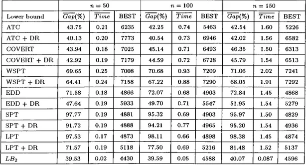
5.8 Linear Lower Bound: Computational Results for n = 50 67

(14)

LIST OF TABLES xii

5.9 Linear Lower Bound: Computational Results for n = 100 . . . . 67

5.10 Linear Lower Bound: Computational Results for n = 150 . . . . 67

5.11 Comparison of Linear Lower B o u n d s ... 68

5.12 Overall Computational Results 68

5.13 The Effect of the New Dominance R u l e ... 68

5.14 Comparison of Emmons’ Rule with the Proposed Rule 69

5.15 Number of Global Dominances for n = 50 69

5.16 Lower Bound {LBi) Value for n = 5 0 ... 69 5.17 Number of Global Dominances for n = 1 0 0 ... 70

5.18 Lower Bound (LBi) Value for n = 100 70

5.19 Number of Global Dominances for n = 1 5 0 ... 71 5.20 Lower Bound (LBi) Value for n = 1 5 0 ... 71

(15)

C hapter 1

In trod u ction

Scheduling is a term in our everyday vocabulary, although we may not always have a good definition of the term in mind. A schedule is a tangible plan or document, it tells us when things will happen, it shows a plan for timing of certain activities and answers the question, “ when will something take place?”. More formally, scheduling may be defined as “the allocation of resources over time to perform a collection of tasks”. Scheduling is a decision making process that exists in most manufacturing and production systems as well as in most information processing environments. It also exists in transportation and distribution settings and in other types of service industries.

The scheduling theory is concerned primarily with mathematical models that is related to the process of scheduling. The development of useful models which leads in turn to solution techniques and insights, has been continuing interface between theory and practice.

The scheduling models are categorized by specifying the resource configura tion and nature of the task. The number of machines, their configuration, i.e. series and parallel, number of jobs, etc. are important aspects in scheduling theory. If the set of jobs available for scheduling does not change over time, the system is called static, in contrast to cases in which new jobs appear over time, where the system is called'dynamic.

(16)

CHAPTER 1. INTRODUCTION

In this study, we consider a single machine scheduling problem. Single machine problems are important for various reasons. The single machine environment is simple and a special case of all environments. Single machine models often display properties that do not hold for either machines in parallel or machines in series. The results that can be obtained for single machine models not only provide insights into the single machine environments, they also provide a basis for heuristics for more complicated machine environments. In practice, scheduling problems in more complicated machine environments are often decomposed into sub-problems that deal with single machines. For example, a complicated machine environment with a single bottleneck may give rise to a single machine model.

A single machine problem is characterized by the following conditions. There is a set of n independent, single operation jobs which are available for processing simultaneously at time zero. The setup times for the jobs are independent of job sequence and included in processing times. The job descriptors, such as due dates, processing times and weights, are deterministic and known in advance. The machine is continuously available and never kept idle while work is waiting. Once an operation begins, it proceeds without interruption.

In general, a schedule specifies when and on which machine each job

i is to be processed. The aim is to find a schedule that optimizes some

performance measure. Performance measures are mainly in two categories: regular performance measures and non-regular performance measures. If a performance measure is non-decreasing in each of the job completion times, it is called a regular performance measure, otherwise it is called non-regular.

The performance measure, “meeting job due dates” , is one of the scheduling criteria most frequently encountered in practical problems. While meeting due dates is only a qualitative goal, it usually implies that time dependent penalties are assessed on late jobs but no benefits derive from completing jobs early. This interpretation leads naturally to the tardiness measure as a quantification of scheduling objective. Tardiness criterion is a regular performance measure;

(17)

it is non-decreasing in each of the job completion times. The difficulty of dealing with this measure arises from the fact that tardiness is not a linear

function of completion times. This means that finding optimal solutions

often requires combinatorial optimization methods. Furthermore because of complexities of combinatorial methods quickly computed suboptimal solutions are also important.

The vast majority of scheduling literature is replete with rules that do not consider job tardiness penalty or customer importance information. As firms struggle to survive in an increasingly competitive environment, a greater emphasis needs to be placed on coordinating the priorities of the firms throughout the functional areas. Firms have a variety of customers some of which are more important than others. The importance of a customer can depend on a variety of factors, such as the firm’s length of relationship with the customer, how frequently they provide business to the firm, how much of the firm’s capacity they fill with orders and the potential of a customer to provide orders in the future. In many applications, meeting due dates and avoiding delay penalties are the most important goals of scheduling. The costs of tardy deliveries, such as customer bad will, lost future sales, and rush shipping costs, vary significantly over customers and orders, and the implied strategic weight should be reflected in job priority. The firm’s strategic priorities thus require the information pertaining to customer importance be incorporated into its shop floor control decisions. In addition, in the presence of job tardiness penalties, it may not be enough to measure the shop floor performance by employing unweighted performance measures alone which treat each job in the shop as equally important.

In this study, the main objective that we consider is the minimization of total weighted tardiness for the static single machine problem. Each job has an integer due date and processing time and positive weights.

We present a new dominance rule for the single machine total weighted tardiness problem with job dependent penalties. The proposed dominance rule provides a sufficient condition for local optimality. We show that if

(18)

any sequence violates the dominance rule, then switching a violating job either lowers the total weighted tardiness value or leaves it unchanged. We also develop an algorithm based on the dominance rule, which is compared to a number of competing heuristics for a set of randomly generated problems. Furthermore, the presented results form a strong background for making adjacent job interchanges so it can be used in reducing the number of alternatives for finding the optimal solution in complete enumeration techniques. We show that having a better upper bound value which is close to optimal solution usually improves the lower bound value which is obtained from Lagrangian relaxation of machine capacity constraints. We also prove that the proposed dominance rule increases the number of global dominances generated by the Emmons’ Rule.

The remainder of the thesis can be outlined as follows. In the following chapter, we give a short review of the literature on total weighted tardiness problem along with the well-known dispatching rules for weighted tardiness problem. In Chapter 3, we discuss the underlying assumptions and give a list of definitions used throughout this thesis. We also discuss the proposed dominance rule along with the transitivity properties. We analyze 16 possible cases to demonstrate our dominance rule. In Chapter 4, we introduce an algorithm which takes its background from the dominance rule we propose and use it for upper bounding scheme. We also present detailed computational

results. We discuss the lower bounding scheme and analyze the effect of

dominance rule on three different lower bounding schemes in Chapter 5. Finally, in Chapter 6, some concluding remarks and suggestions for future research are provided.

(19)

C hapter 2

L iterature R eview

Sequencing and scheduling are forms of decision making which play a crucial

role in manufacturing as well as in service industries. Scheduling is the

allocation of resources over time to perform a collection of tasks. The

sequencing problem is a specialized scheduling problem in which we establish an ordering of jobs for each work center. In the current competitive environment, effective sequencing and scheduling has become a necessity for survival in the market place. Companies have to meet shipping dates committed to the customers, as failure to do so may result in significant loss of good will. They also have to schedule activities in such a way as to use resources available in an efficient manner.

Scheduling began to be taken seriously in manufacturing at the beginning of this century with the work of Henry Gannt and other pioneers. However, it took many years for the first scheduling paper in the operations research

literature to appear. Some of these first publications appeared in Naval

Research Logistics Quarterly in the early 1950s and contained results by W.E. Smith [43], S.M. Johnson [24] and J.R. Jackson [21]. During the 1960s, a significant amount of work was done on dynamic programming and integer programming formulations of scheduling problems. After Richard Karp’s [25] famous paper on complexity theory, the research in the 1970s focused mainly on the complexity hierarchy of scheduling problems. In the 1980s, several

(20)

CHAPTER 2. LITERATURE REVIEW

different directions were pursued in academia and industry with an increasing amount of attention paid to stochastic scheduling problems. Also, as personal computers started to permeate manufacturing facilities, scheduling systems were being developed for the generation of usable schedules in practice. This system design and development was, and is, being done by computer scientists, operation researchers, and industrial engineers.

Over the last three decades, a number of books on sequencing and scheduling have appeared. These books range from the elementary to the more advanced. One of the known textbooks is Conway, Maxwell and Miller [8] (it seems to be out of date but it is still interesting). A more recent text by Baker [4] gives an excellent overview of many aspects of deterministic scheduling. However, in the first edition [3], there is no complexity issues since it appeared just before research in computational complexity became popular. An introductory textbook by French [14] covers most of the techniques that are used in deterministic scheduling. The proceedings of a NATO workshop, edited by Dempster, Lenstra, and Rinnooy Kan [9], contains a number of advanced pcipers on deterministic, as well as stochastic scheduling. The more applied text by Morton and Pentico [35] presents a detailed analysis of a large number of scheduling heuristics that are useful for practitioners. One of the most recent textbooks by Pinedo [36] deals with deterministic and stochastic models with applications so that the relevance of the theory to the real world can be found.

Besides these books, a number of survey articles have appeared, each one with a large number of references. We mention the review by Graves [17], the introductory survey of precedence constrained scheduling by Lawler and Lenstra [30], the tutorial on one machine scheduling by Lawler [29], the NP-completeness column on multiprocessor scheduling by Johnson [23], the annotated bibliography covering the period 1981-1984 by Lenstra and Rinnooy Kan [33], the discussions of new directions in scheduling by Lenstra and Rinnooy Kan [32] and an overview of single machine sequencing by Gupta and Kyparisis [19]. Lawler, Lenstra, Rinnooy Kan, and Shymoys [31] give a detailed overview of deterministic sequencing and scheduling.

(21)

A scheduling problem is described by a triplet oi\II\'). The a field describes

the machines environment and contains a single entry. The ^ field provides details of processing characteristics and constraints and may contain no entries, a single entry, or multiple entries. The 7 field contains the objective to be minimized and usually contains a single entry. For the a field, single machine, identical machines in parallel, machines in parallel with different speeds, unrelated machines in parallel, flow shops, flexible flow shops, open

shops and job shops, are examples. For the (I field, possible entries are

release dates, sequence dependent setups, preemptions, blocking, no wait and recirculation. For the 7 field, lateness, tardiness, makespan, maximum lateness, total weighted completion times, discounted total weighted completion times, total weighted tardiness and weighted number of tardy jobs can be good examples.

In this study, we consider single machine total weighted tardiness problem, i.e. 1| I Y^WiTi. Weighted tardiness function is a well known due date related penalty function and a considerable amount of work has been done in literature.

One of the first results in tardiness scheduling is the well known Elmaghraby lemma ([10]). Given a set S of unscheduled jobs which are available at time zero, if there is a job k ^ S such that dk > YiesPi 1-hen there exists an optimal schedule in which k is the last among all jobs in S. Since k will never be tardy if we process it last among the jobs in hand, the job can be removed from the problem.

Another important study is Emmons’ [11] paper in which he derives several dominance rules that establish the relative order in which pairs of jobs are processed in an optimal sequence to restrict the search for an optimal solution for total tardiness problem. He establishes some corollaries which can be used for more general criterion of minimizing sum of identical, convex, non decreasing functions of job tardiness. Later, Rinnooy Kan et al. [41] extended these results to the weighted tardiness problem. Such dominance tests can be used to structure the problem as a global precedence network. As a result of Emmons’ Theorem two corollaries can be stated: Shortest processing time

(22)

(SPT) sequence gives optimal for the total tardiness problem if it yields a sequence where all jobs are tardy. Similarly for the total weighted tardiness IDroblem, weighted shortest processing time (WSPT) sequence gives the optimal when all jobs are tardy. Furthermore, earliest due date (EDD) sequence which emphasizes job urgency by using the global due date di is optimal if it yields a sequence where at most one job is tardy.

Lawler [27] as well as Lenstra et al. [34] show that the total weighted tardiness problem, 1] \J2wiTi, is strongly NP-hard. The proof is done by reducing the 3-PARTITION problem to 1] j Y^WiT problem. Lawler also gives a pseudo polynomial algorithm for the total tardiness problem, Ij ¡ Y T . He develops a theorem which is also applicable to the weighted tardiness case. Although this theorem is not for finding precedence relations, it gives some decomposition principles. Decomposition refers to dividing the problem into

smaller sets which can be solved separately. The decomposition theorem

of Lawler assumes that jobs are in EDD order and then finds alternative decompositions which result moving the longest unscheduled jobs to different places. In order to find the optimal sequence, all alternative decompositions must be carried on. Lawler [26] also shows that a relaxation of the total weighted tardiness problem can be formulated as a transportation problem.

Szwarc [45] proves the existence of a special ordering for the single machine earliness-tardiness problem with job independent penalties where the arrangement of two adjacent jobs in an optimal schedule depends on their start time. He shows that each pair of adjacent jobs has a critical start time (which we call breakpoint) after which the precedence relationship changes direction. He shows the existence of critical time points for both total tardiness problem and weighted tardiness problem [46] when tardiness penalties are proportional to the processing times . Szwarc and Liu [46] present a two-stage decomposition mechanism to 1 ] \ Y WiTi problem when tardiness penalties are proportional to the processing times which proves to be powerful in solving the problem completely or reducing it to a much smaller problem. As stated by Jensen et al. [22], the importance of a customer can depend on a variety of factors, such as the firm’s length of relationship with the customer, how frequently they

(23)

provide business to the firm and the potential of a customer to provide orders in the future. Therefore, we present a new dominance rule for the most general case of total weighted tardiness problem.

Various enumerative solution methods have been proposed for both the weighted and unweighted cases of the total tardiness. Emmons’ rules are used in both branch and bound (B&B) and dynamic programming algorithms (Fisher [12] and Potts and Wassenhove [37] [38]). Rinnooy Kan et al. [41] and Schräge and Baker [42] extended these results for more general objective functions. Rachamadugu [39] identifies a condition characterizing adjacent jobs in an optimal sequence for 1] \ Y,WiTi. This condition can be used as a pruning device in enumerative methods. Abdul-razaq and Potts [2] consider the problem where the costs are no longer assumed to be nondecreasing functions of completion time. Chambers et al. [7] develop new heuristic dominance rules and a flexible decomposition heuristic.

For the exact solution methodologies various lower bounds have been proposed. Rinnooy Kan et al. [41] use a linear assignment relaxation based on an underestimate of the cost of assigning job i to position fc, and Gelders and Kleindorferer [15] [16] develop a lower bound based on the relaxation of a similar transportation problem. Fisher [12] proposes a method in which the requirement that a machine can process at most one job at a time is relaxed. In this approach, one attaches ’prices’ (i.e. Lagrangian multipliers) to each unit time interval and looks for the cheapest schedule that does not violate the cajracity constraint. Sousa and Wolsey [44] present a time indexed formulation of this problem, which gives better lower bounds than other mixed integer programming formulations. Hoogeveen and Van de Velde [20] reformulate the problem by using slack variables to obtain stronger lower bounds. They show that better Lagrangian bounds can be obtained by addressing the slack variable problem that results from reformulating nasty inequality constraints as equality constraints. The improved Lagrangian lower bound is set equal to the traditional bound plus the bound on the slack variable problem.

(24)

CHAPTER 2. LITERATURE REVIEW 10

obtains lower bounds using a Lagrangian relaxation approach with subproblems that are total weighted completion time problems. Since the well-known sub gradient optimization method is time consuming, they replace it by a multiplier adjustment method that leads to an extremely fast but rather weak bound calculation. The method incorporates various devices for checking dynamic programming dominance in the search tree. The approach contradicts the often heard conjecture that one should restrict the search tree as much as possible by using the sharpest possible bounds.

The exact approaches used in solving the weighted tardiness problem are

tested by Abdul-razaq et al. [1] and they use Emmons’ dominance rules

to form a precedence graph. The dynamic programming algorithms use

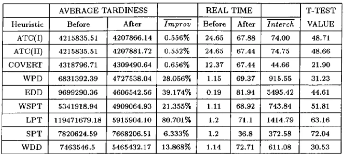
the same recursion defined on sets of jobs, but they generate the sets in lexicographic order (Schrage-Baker [42]) and cardinality order (Lawler [28]) resj^ectively. The branch and bound algorithms use lower bounds based on transportation problem (Lawler [26]), a linear assignment relaxation (Rinnooy Kan et al.[41]), Lagrangian relaxation (Fisher [12]), dynamic programming state space relaxation (Abdul-razaq and Potts [2]) and reduction of total weighted tardiness problem to total weighted completion time problem i.e. linear and exponential lower bounds proposed by Potts and Wassenhove [37]. The branch and bound algorithm which obtains a lower bound from a linear function of completion times problem is the most efficient and is able to solve problems up to 40 jobs. Abdul-razaq et al. [1] show that the most ¡Drornising lower bounds both in quality and time consumed are the linear and exponential lower bounds which are obtained from Lagrangian relaxation of machine capacity constraints proposed by Potts and Wassenhove [37]. The computational results show that the linear lower bound is superior to exponential lower bound.

Since the implicit enumerative algorithms may require considerable computer resources both in terms of computation times and memory, several heuristics and dispatching rules are proposed. Large scale problems are usually treated with heuristic procedures called dispatching or sequencing rules. These are logical rules for choosing which available job to select for processing at a

(25)

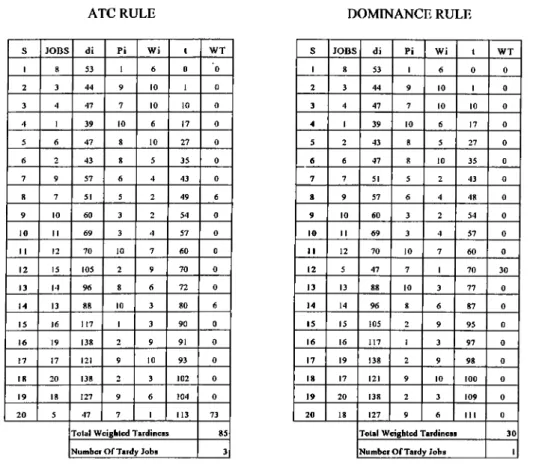
particular work center. In using dispatching rules, usually scheduling decisions are made sequentially rather than once. For the static dispatching rules, the job priorities does not change over time while priorities might change over time for the dynamic dispatching rules. A list of dispatching rules is given in Table 2.1. In this table, the EDD, LPT, SPT, WSPT, WDD and WPD are examples of static dispatching rules, where as АТС and COVERT are dynamic ones.

The WSPT rule, using the ‘natural priority’ of job i, Wilpi^ or the penalty avoided, works analogously to the SPT rule, such that overall tardiness is reduced in congested shops by giving priority to short jobs and Wi helps in coordinating job priorities. By delaying some long jobs, WSPT can also achieve a remarkably low total number of tardy jobs without using explicit due date information, especially when job earliness is limited by dynamic release dates. WSPT rule gives an optimal sequence when all release dates and due dates are zero.

Vepsalainen and Morton [47] develop and test efficient dispatching rules for the weighted tardiness problem with specified due dates and delay penalties. Carroll [6] designed a dynamic rule for average tardiness scheduling to be used to incorporate job weights into a slack based approach. The COVERT priority index represents the expected tardiness cost per unit of imminent processing time, or cost per unit of imminent processing time, or Cost OVER Time. Under COVERT Rule, jobs are scheduled one at a time; that is, every time the machine becomes free, a ranking index is computed for each remaining job i. The job with the highest ranking index is then selected to be processed next. The ranking index is a function of the time t at which the machine became free as well as the pi, the Wj, and the d,· of the remaining jobs. The index for COVERT can be defined as:

U\ rn 1 m a x ( 0 , d i - i - P i )

7ri[t) = max (— max[0 ,1 --- ---^J)

Pi ^Pi

.Job i queuing with zero or negative slack is projected to be tardy by completion with an expected tardiness cost Wi and priority index Wijpi. k is the look ahead parameter and is set to 2. The original results proved COVERT superior to the competing rules, including a truncated SPT, in mean tardiness performance

(26)

(Carroll [6]).

The apparent tardiness cost (АТС) heuristic is a composite dispatching rule that combines the WSPT rule and the minimum slack (MS) rule. Under the АТС rule, the index can be defined as:

, — max (0 , di — t — pi).

Wi

TTi{t) --- exp

(-Pi к ■ p ■)

where we set the look-ahead parameter at 2 as suggested by Morton and

Pentico [35], and p is the average processing time. Vepsalainen and Morton [47] have shown that the АТС rule is superior to other sequencing heuristics and close to optimal for the Ijj Y^WiTi problem. It trades off job’s urgency (slack) against machine utilization, but due to the more complex weighted criterion, an additional look ahead parameter is needed to assimilate the competing jobs which have different weights. In computational tests which is done by Rachamadugu and Morton [40], an exponential function of the slack was found to be somewhat more efficient. Intuitively, the exponential look ahead works by ensuring timely completion of short jobs (steep increase of priority close to due date), and by extending the look ahead far enough to prevent long tardy jobs from overshadowing clusters of shorter jobs. The АТС and COVERT rules outperformed the competing rules even with fixed average parameter values, and contrary to practitioners’ previous suspicion, improving adjustments can be made for extreme load conditions on the basis of expected queue lengths.

Now, we can present some preliminary results stated by Morton and Pentico [35] for the static total weighted tardiness (TUi) problem which is known to be a difficult problem. These rules can help us for learning much about the optimal solution. Now, let’s give the results:

• If any sequence produces T^t — 0, then EDD is optimal.

• If all jobs have same due date, T^t is minimized by WSPT if either all weights are equal or Pi = 1.

• If WSPT makes all jobs tardy then Ty^t is minimized by WSPT if either

(27)

• If no possible sequence can make any job non tardy then Tyjt is minimized by WSPT.

• If a job is not tardy when scheduled second instead of first then it need not be scheduled first.

• If the job with the highest WSPT priority is tardy even if scheduled first, then it should be scheduled first.

These propositions can effectively be used in heuristic scheduling and the dispatching rules in the literature are developed by using the intuition behind these propositions.

The weighted tardiness problem is NP-hard and the lower bounds in the literature are either weak or not practical to use due to extensive computational requirements. The exact solutions usually rely on Emmons’ dominance rules for lower bounding schemes to restrict the search space. As a result, the exact solution for a 50 job problem is a barrier that could not be passed. Therefore, we present a new dominance rule for the most general case of total weighted tardiness problem. The proposed rule provides the sufficient condition for local optimality, and it generates schedules that cannot be improved by adjacent job interchanges. We also propose an algorithm to demonstrate how the proposed dominance rule can be used to improve a sequence given by a dispatching rule. We show that if any sequence violates the proposed dominance rule, then switching a violating job either lowers the total weighted tardiness or leaves it unchanged.

Abdul-razaq et al. [1] show that the linear lower bound proposed by Potts and Wassenhove [37] is superior to all other lower bounds. The linear lower bound calculations are based on an initial sequence, therefore we test the impact of quality of initial solution on the quality of lower bound value obtained in Chapter 5. Since the dominance rule proposed either lowers or leaves the upper bound value unchanged, our expectation is having a better lower bound Vcilue when a sequence generated by the dominance rule is used for the linear lower bound. We also test how the number of global dominances affects the

(28)

RULE DEFINITION RANK and PRIORITY INDEX

ATC Apparent Tardiness Cost max (m exp (

COVERT Weighted Cost Over Time m a x ( a m a x [ 0 . 1 - ” “ <°g-->")|)

WPD Weighted Processing Due date _&

EDD Earliest Due Date min (di)

WSPT Weighted Shortest Processing Time max ( ^ )

LPT Longest Processing Time max (pi)

SPT Shortest Processing Time min (pi)

WDD Weighted Due Date m a x ( f )

Table 2.1: Dispatching Rules in Literature

lower bound value. We compare Emmons’ and the proposed dominance rules on a lower bound which uses global dominance information generated by these rules. In Chapter 6, after making a short summary, we give some concluding remarks along with the future directions.

(29)

C hapter 3

D om inance R ule

A dominance property is any property that specifies a subset of the set of sequences which can be guaranteed to contain an optimal sequence. Dominance properties provide conditions under which certain potential solutions can be ignored. The computational demands for the exact solution grow exponentially with problem size. Restricting attention to the dominant set reduces the number of alternatives therefore the computational effort involved in searching an optimal solution decreases.

In this chapter, we give dominance rules and transitivity properties for the total weighted tardiness problem. We show that the arrangement of adjacent jobs in an optimal schedule depends on their start times. For each pair of jobs,

i ci.nd j , that are adjacent in an optimal schedule, there can be a critical value tij such that i precedes j if processing of this pair starts earlier than t{j and j

precedes i if processing of this pair starts after tij.

This chapter is organized as follows: In §3.1, the problem definition and the notation used are given. In §3.2, the dominance rule is explained by examining sixteen possible cases and finally, in §3.3, the transitivity properties for total weighted tardiness problem are introduced.

(30)

CHAPTER 3. DOMINANCE RULE 16

3.1 P ro b lem D efin itio n and N o ta tio n

The single machine total weighted tardiness problem, 11 | WiT, may be stated

as follows. Each of n jobs (numbered is to be processed without

interruption on a single machine that can handle only one job at a time. Job

i becomes available for processing at time zero. It has an integer processing

time Pi, a due date di and has a positive weight Wi. For convenience the jobs are arranged in an EDD indexing convention such that d, < dj, or di = dj then Pi < pj, or di = dj and pi = pj then Wi > Wj for all i and j such that i < j. The problem can be formally stated as: find a schedule S that

minimizes f { S ) — WiTi. To introduce the dominance rule, consider

schedules Si = QiijQ^ and S2 = Q ij iQ2 where Qi and Q2 are two disjoint

subsequences of the remaining n — 2 jobs. Let t = Pk be the completion

time of Qi- Define Ti(t) as the total weighted tardiness of job i if scheduled at time t and Tij(t) be the total weighted tardiness of jobs i and j if i precedes j cind their processing starts at time t. Then, Ti{t) = Wima,x{Q,t + Pi — di) and

Tij(t) = tVi max(0, t + p,· — di) + Wj max(0, i + pi + pj — dj).

The following interchange function, A ,j(i), is used to specify the new dominance properties, which gives the cost of interchanging adjacent jobs i and j whose processing starts at time t.

Aijit) - Tji{t) - Tij{t) = Wj max(0, t-\-pj - dj) + Wi max(0, i + p*· + pj - d{) —Wi max(0, t Pi — di) — Wj max(0, t A pi -\- pj — dj)

Note that this cost Aij{t) does not depend on how the jobs are arranged in Qi

and Q2 but depends on start time t of the pair, and

• if Aij{t) < 0 then, j should precede i at time t. • if Aij{t) > 0 then, i should precede j at time t.

• if Aij{t) = 0 then, it is indifferent to schedule i or j first.

(31)

Breakpoint is a time in which it is indifferent to schedule either i or j first

and for t < breakpoint, i precedes j (or j precedes i) and then j precedes i (or

i precedes j).

A breakpoint is valid if it is in the specified interval.

The ordering is said to be transitive if for any three jobs i, j and k, i precedes j and j precedes k then i precedes k holds.

i globally precedes j , i j , {j globally precedes i, j => i) if it implies the

existence of an optimal sequence in which job i (job j ) precedes job j (job i) is guaranteed and the global transitivity property holds.

i unconditionally precedes j , {i —> j) if there is no breakpoint so the

ordering does not change, but the transitivity property might not hold. Thus it does not imply that an optimal sequence exists in which i precedes j.

i conditionally precedes (i -< j ) if there is at least one breakpoint between

the pair of jobs. The order of jobs depends on the start time of this pair and changes in two sides of that breakpoint.

When all of the possible cases are studied, it can be seen that there are at most three possible breakpoints as shown below.

'^idi '^jdj f

{Pi+pj) (3.1)

= dj - p i - Pj(l - Wi/Wj) (3.2)

^ d i - pj - pi{l - Wj/wi) (3.3)

3.2 D o m in a n ce R u le

The proposed dominance rule takes its background from the adjacent pairwise interchange method, which can be used to improve the total weighted tardiness criterion of a given sequence. If the problem is known to be convex, this method might lead to an optimal solution. But the discrete optimization problems such

(32)

as scheduling problems are often not convex, so only a local improvement can be made. However, a pairwise interchange preceded by a good heuristic has a reasonable chance to lead to optimal solution. Furthermore, we will show that if any sequence violates the proposed dominance rule, then switching a violating job either lowers the total weighted tardiness or leaves it unchanged. The proposed rule provides a sufficient condition for local optimality, and it generates schedules that cannot be improved by adjacent job interchanges.

After giving the intuition behind the adjacent pairwise interchange method, sixteen different combinations of pi vs. pj, Wi vs. wj, d j —di vs. pj, and di~pi vs.

dj —pj are presented below and we analyze the interchange function ¿^ij{t) for

each case. As a result, three breakpoints are found and transitivity properties cire shown for certain instances.

1. di < d j , Pi p j , di — p i < d j — p j 4. d i < d j . Pi W j , d j - d i W j , d j — di d j — p j 6. d i < d j . Pi Wj , d j - d i > p j , di - p i < d j - p j 7 . di ^ Pi ^ Pj^ "î ^ î ^ Pj^ î Pi — Pj 8. di ^ d j , Pi ^ P j , Wi ^ 5 d j di p j, d^ p i ^ d j p j 9. d i < d j . Pi > P j , Wi > W j , d j - d i P j , Wi > W j , d j - d i > p j , di - p i < d j - p j 1 1 . di < d j . Pi p j , d i - p i > d j - p j 12 . d i < d j . Pi W j , d j - d i > p j , d i - p i > d j - p j 13. d i < d j . Pi > P j , Wi < W j , d j - d i d j - p j

(33)

CHAPTER 3. DOMINANCE RULE 19 d j - P i - P j d . - P i - P j d j - P j d.-p. --- 1--- ^--- 1---^— d: ^ time A B c D E Figure 3.1; di < dj, pi < pj, dj — di < pj and di — pi < dj — pj 14. di < dj, Pi > Pj, Wi < Wj, dj — di > pj, di — pi > dj - pj 15. di < dj. Pi > Pj, Wi > Wj, dj — di < pj, di - pi > dj — pj 16. di < dj. Pi > Pj, Wi > Wj, dj — di > pj, di — pi > dj — pj 3.2 . 1 di < d j , Pi < P j , Wi < W j , d j — di < p j , di — Pi < d j — p j

First, let’s investigate how Aij(t) changes in this case. As it can be seen from Figure 3.1, there are 5 regions to examine:

1. In region A, ( t ^ di — [pi + Pj)) no tardiness occurs, so it is indifferent

to schedule either i or j first.

2. In region B, ( di — (pi +Pj) < t < dj — (pi +Pj)), i is tardy if not scheduled first. Here, Aij{t) = Wi{t+pi+pj-di). Since di~{pi+pj) < t, Aij{t) > 0 so i ^ j.

3. In region C, {dj — (pi + pj) < t < di — pi), either i or j is tardy if not scheduled first. Here, Aij(f) = {wi — Wj)t + {pi+pj){wi — Wj) — Widi + Wjdj.

The breakpoint t}j = — {pi + Pj)) is defined in this region. If

the processing of this pair starts up to f < tjj then i ^ j and j X i if

processing begins after t]j.

4. In region D, {di — pi < t < dj — pj), i is always tardy but j is not tardy

if scheduled first. Here, Aij{t) = WiPj — Wjt — Wj{pi + pj - dj). There is

a new breakpoint t]j — dj — pi — Pj{l — Wifwj). Similar to above, i ^ j

(34)

5. In region E, ( dj —pj < t) both jobs are tardy. Here, Aij{t) = WiPj — WjPi. If Aij(t) > 0 then i -< j , otherwise j ■< i.

It seems that there is more than one breakpoint, but actually as we are going to show below at most one breakpoint can be valid, i.e. it is in the specified region of either C or D for t]· and tfj, respectively, and up to that breakpoint

i ^ j and then j ^ i. If there is no valid breakpoint then i unconditionally

precedes j , i.e. i ^ j.

We will derive the following equations in order to show that at most one breakpoint can be valid. If tfj < dj — pj then from equation (3.2):

Pi > Pji'Wilwj) Pi = pjiwijwj) + for > 0 (3.4) If t\j < di — Pi, i.e. valid then from equation (3.1) after some algebraic manipulations:

di > dj — Pj + pj{wifwj) di = dj — pj{l — Wijwj) + for > 0 (3.5) Observe that if tfj > di — pi then from equation (3.2):

di < dj - Pj + pj{wifwj) = > di - dj - pj{l - Wilwj) - for > 0 (3.6) So we can say from equations (3.5 & 3.6) that both breakpoints cannot be valid cit the same time. With simple algebra.

• if t}j < tL then

i.e. t]j < di - Pi • if > *lj

i.e. t'ij > di — Pi.

di > dj - pj{l - Wifwj) (3.7)

di < dj — pj{l — Wi/wj) (3.8)

So if tij is valid then t]j < tL and similarly if i?· is valid then t}j > t}j. So we can deduce the following proposition from all equations above:

(35)

P ro p o s itio n 1 I f there is a valid breakpoint then it is )

P ro o f: Follows from equations (3.5, 3.6, 3.7 &: 3.8). □

The following proposition is useful when both of the breakpoints are invalid.

P ro p o s itio n 2 Ift}j and tf- are both invalid then i

P ro o f: From equations (3.4, 3.5 L· 3.6), it is known that if both of the breakpoints are invalid then tjj > tfj > dj — pj.

• In region B, we know that Ajj(i) > 0. So i -< j.

• For dj - (pi+pj) < t < d i - Pi, Aij{t) = {wi - Wj)t + {pi + pj){wi - Wj) - Widi + Wjdj. Since t}j is invalid tjj > di—pi, so dj = d j+ p j(l — Wi/wj) —

= > Aij{t) - {wi-Wj)tp{pi-{-pj){wi-Wj)-Widi-\-Wj{diTpj{l-Wilwj)-e^

Aij{t) - {wi - Wj){t - {di - Pi)) + Wit^.

Since {wi — Wj) < 0, (i — {di — pi)) < 0 and > 0 then Aij{t) > 0. So

i X j.

• For di - p i < t < dj - Pj, Aij{t) = WiPj - Wjt - Wj{pi+pj - dj). Since t}j

and tfj are both invalid, tfj > dj — pj so pj — pi{wj/wi) + e^, for > 0.

= > Aij{t) = wi{pi{wjfwi) + e^) - Wjt - Wj{pi + pj - dj) Aij{t)

-WiC^ — W j { t — { d j — P j ) ) . Since { t — { d j — p j ) ) < 0, then A i j { t ) > 0. So i ■< j.

• for dj — Pj < t, Ai j {t ) = w'iPj — WjPi. Since tL > dj — pj = > Ai j {t ) > 0. So i -< j.

The result follows, if both ¿h and tf- are invalid then i —* j . □

The Propositions 3 and 4 can be used to specify the order of jobs at time t.

(36)

P ro o f: To show that we have to examine the regions D and E as follows:

• For di — Pi < t < dj — pj, A.ij{t) — WiPi — Wjt — Wj{pi + pj — dj). Since /h is valid from equation (3.5), dj = d, + p j(l — Wifwj) — e^.

= > Aij{t) = Wj{di — Pi — t — e^) + Wi{pi — Pj). Since t > di — pi and

Pi < Pj., < 0 which means j -< i.

• For dj — Pj < t, Aij(t) = WiPj — WjPi. Since tfj < dj — pj, i.e. t}j < tfj < di — Pi < dj — Pj, from equation (3.4) we have WiPj — WjPi < 0, or Aijit) < 0, so j -< i.D

P ro p o s itio n 4 Ift]j is valid then up to tjj, i < j and then j -< i.

P ro o f: Proof is similar to the proof of Proposition 3.Q

T h e o re m 1 There can be at most one valid breakpoint for this case, i.e.

mm{tij,tfj), and if t}j and tfj are both invalid then i j .

P ro o f: Follows from Propositions 1, 2, 3 and 4.D

The following rule summarizes the results of the first case.

R u le 1 U t}j is valid then,

for t < t]j, i j. then j ^ i else iftfj is valid then,

for t < t } j , i A j , then j A i else i

(37)

CHAPTER 3. DOMINANCE RULE 23 d i - P i - P j d j - P i - p j dj-Pj dj-Pi -l·- time A B c D E Figure 3.2: di < dj^ pi < pj, dj — d{ < pj and d{ — Pi > dj — pj 3.2 . 2 di < d j , Pi d j — p j

We will start again by investigating how Ajj(i) changes in this case. As it can be seen from Figure 3.2, there are 5 regions to examine, but regions A, B and E are same with the previous case 3.1, so only regions C and D are examined below.

1. In region C, (dj — {pi + pj) < t < dj — pj), either i or j is tardy if not scheduled first. Here, Ajj(f) = {wi — Wj)t + {pi+pj){wi — Wj) — Widi + Wjdj. Similar to the previous case, we have the breakpoint tjj in this region. Therefore, i -< j for t < tjj, and j -< i afterwards.

2. In region D, {dj — Pj < t < di — pi), j is always tardy but i is not tardy if scheduled first. Here, Ajj(i) = —Wjpi + Wi{t + pi + pj — di). There is a new breakpoint i?· = di — pj — Pi{l — Wjfwi). If it is a valid breakpoint then for t < tL, j ^ i and then i -< j.

As shown above, there can be two breakpoints for this case. We will derive the following equations to show that i?· depends on tjj.

If iij < dj — Pj (i.e. valid) then from equation (3.1):

dj — di < pi{wj/wi — 1) dj — di < pi{wjfwi — 1) — for > 0 (3.9) If tf· > dj — Pj then from equation (3.3):

dj — di < pi{wj/wi — 1) dj - di < pi{wjfwi — 1) — for > 0 (3.10)

So from equations (3.9 L· 3.10), if t]j is invalid then is also invalid.

If tL < di — Pi then from equation (3.3):

(38)

P ro p o sitio n 5 I f tL is valid then tjj is also valid. I f t]j is valid and is invalid then tfj > di — pi.

Proof: Follows from equations (3.9, 3.10 L· 3.11).D

Proposition 6 shows how Aij(t) changes if both of the breakpoints are valid.

P ro p o sitio n 6 I f both breakpoints are valid then for t < t]·, i -< j , for tjj <

t < j -< I o-'f^d for tL < t, i ^ j .

Proof: The only region that should be examined is region E, since Aij{t)

remains same in other regions. Aij(t) — WiPj — wjpi and from equation (3.11) it is known that piWj < PjWi, i.e. Aij(t) > 0, so i -< j.O

Proposition 7 demonstrates how Aij{t) changes if fb is the only valid breakpoint.

P ro p o sitio n 7 Iftjj is valid and tL is invalid f o r t < tjj, i -< j and then j -< i.

Proof: From equations (3.9, 3.10 & 3.11), i?· > d, — pi ==^ pi = pjWifwj +

for > 0. So in region D,

Aij{t) = -WjPj(wi/wj) - Wjt^ - Wi{t + Pi + pj - di). Aij{t) = -WjC^ + Wi{t + Pi - di)

==^ Aij{t) < 0, so j -< i. In region E, Aij{t) = WiPj — WjPi < 0, so j ^ i . □ The following proposition shows how Aij{t) changes if both of the breakpoints are invalid.

P ro p o sitio n 8 I f tjj is invalid then i j .

Proof: If we can show that i -< j in all regions then i —>^j. tjj is invalid so tjj > di - Pi and

(39)

• In region C, Ai j ( t ) = (tOi ^ Wj)t + (pi + pj)(wi - wj ) - Widi + Wjdj. From equation (3.12),

Aij{t) - {wi - Wj)t + {pi -\-pj){wi - Wj) - Wi{dj-piiwjfwi - 1 ) - e'^) + Wjdj.

Aij(t) — (wi - Wj)(t - dj + Pj) + WiC Aij{t) > 0, so i -< j.

• In region D, Aij(t) = —WjPi — Wi(t + pi + pj — di). From equation (3.12),

Aij(t) = -WjPi - Wi(t + Pi + Pj - {dj - Pi{wjfwi - 1) - e'*))

= Wi(t - dj + Pj + e^)

Aij{t) > 0, so z j.

• In region E, di — Pi < t and Aij{t) = WiPj — WjPi. Since tfj > di — pi,

then Wi P j — Wj P i > 0 and A i j { t ) > 0, so i -< j. □

T h eorem 2 At most two breakpoints can be valid. I f both are valid then for t < tjj, i < j and for t]j < t < tL, j -■ j .

Proof: Follows from Propositions 5, 6, 7 and 8.D

R u le 2 I f ti j is valid then. if tL is valid for t < t}j, i ^ j for t]j < t < Cij, j ^ i and for tfj < t, i ^ j else for t < t]j, i j and for t}j < t, j ^ i else i j .

(40)

CHAPTER 3. DOMINANCE RULE 26 dj-Pi-Pj dj-Pj dj-Pi-Pj --- 1--- ^ ^ ---d: _‘•j-Pj — I— . time A B C D E Figure 3.3: di < dj, pi < pj, dj — di < pj and di — pi < dj — pj 3.2 . 3 di < d j , Pi p j , di — p i < d j — p j

First, let’s investigate how changes. As it can be seen from Figure 3.3,

there are 5 regions to examine but the regions A and E are same with the regions A and E of case 3.2.1, so only regions B, C and D are examined below.

1. In region B, ( di — (pi+Pj) < t < di — pi), i is tardy if not scheduled first. Here, Aij(t) = Wi(t + pi + pj — di). Since di - (pi + Pj) < t, Aij(i) > 0 so

i j.

2. In region C, {di — pi < t < dj — {pi + Pj)), i is always tardy but j is not

tardy. Here, Aij{t) = WiPj. Since WiPj > 0, i j.

3. In region D, ( d j — { p i + Pj) < t < d j — p j ) , i is always tardy but j is not

tardy if it is scheduled first. Here, A i j { t ) — Wi P j — W j { t A p i + p j — d j ) .

There is a breakpoint t L = { d j — p i — pj { l — W i f w j ) here. If it is valid

then for t < t f j , i -< j and then j -< i.

We will show that there might be only one valid breakpoint for this case, which is tjz._‘J

L e m m a 1 The only breakpoint that can be valid is tfj. I f it is valid then i A j

for t < tfj, and j A i afterwards. I f there is no valid breakpoint then always ■I ^ J .

P ro o f: If tfj is valid (i.e. tf- < d j —pj WiPj — WjPi < 0) then for t > d j —pj, Aij{t) — WiPj — WjPi = A Aij{t) < 0, so j A i in region E.

(41)

<^j - (Pi + Pj) < t < d,j - Pj, - WiPj - Wj(t + Pi + Pj - dj). Since

Wipj - WjPi > 0

P j = ( Pi ^ j / ' < J ^ i ) + f o r > 0 ·

A i i ( t ) = W i i { p i W j / w i ) + e ' * ) - W j { t + Pi + P j - d j ) = - W j { t - \ - p j - d j ) + Wic"^

= > Aij(t) > 0, so i -< j.

In region E, i > dj — pj, WiPj — WjPi > 0 ^ij{t) > 0 . So i ^ j . □

T h eorem 3 There can he one valid breakpoint, tfj. I f t]j is valid then up to t'jj, i -< j and then j ^ i. I f there is no valid breakpoint then i j .

R u le 3 I f tL is valid then,

for t < t]j, i ^ j .

and for t > tL, j -< i else always i j .

3 .2 .4

di < d j , Pi W j , d j — di < p j , di — p i < d j — p j

This case is similar to case 3.2.1 (Figure 3.1), but the only difference is Wi > Wj. Notice that, in region C, Ajj(t) = {wi—Wj)t+{pi+pj)[wi—Wj) — Widi+Wjdj > 0

and the breakpoint tjj = — (Pi + Pj)) < 0. Therefore it is not valid.

The second breakpoint t^ is defined in region D. tL is invalid too, since the minimum value that it can get is dj — pi. So there is no valid breakpoint.

L e m m a 2 None of the breakpoints is valid, so i j . (The global transitivity

property holds here, so there is a global dominance)

R u le 4 i globally precedes j . (i ^ j )

3 .2 .5

di < d j . Pi W j , d j — di > p j , di — p i < d j

—

p j

This case is similar to case 3.2.2 (Figure 3.2), except Wi > Wj. Notice that

(42)

invalid too since i?· = di — pj — pi{l — Wjiwi). Lemma 2 and Rule 4 are also applicable here.

3 .2 .6

di < d j , Pi < P j , Wi

>

W j , d j — di > p j , di — p i < d j — p j

This case is similar to case 3.2.3 (Figure 3.3), except Wi > Wj. There is no valid breakpoint for this case either since tL = dj — pi — P j(l — Wifwj) > dj — Pi >

dj — Pj. Lemma 2 and Rule 4 are also applicable here.

The global dominance property for cases 3.2.4 to 3.2.6 is already shown by Emmons. However, Emmons’ dominance rules do not consider the other cases so the precedence graph generated by the proposed dominance rule will contain the graph generated by Emmons’ rules.

3 .2 .7

di < d j , Pi > P j , Wi < W j , d j — di < p j , di — p i < d j — p j

This case is similar to case 3.2.1 (Figure 3.1). It seems that there is more than one breakpoint. But actually as we have shown in §3.2.1, at most one breakpoint can be valid, and up to that breakpoint i -< j then j -< i. If there

is no valid breakpoint then i j. Theorem 1 and Rule 1 are applicable here.

3 .2 .8

di < d j . Pi > P j , Wi < W j , d j — di > p j , di — p i < d j — p j

This case is similar to case 3.2.3' (Figure 3.3). The range of breakpoint

tfj — dj — Pi — Pj{l — Wifwj) is between dj — {pi APj) < tL < dj — Pj, therefore t]· is always valid.

L em m a 3 The breakpoint tfj is always valid. For t < tfj, i -< j and then j A i.