The effect of temperature on the formation of liesegang patterns of copper(II) chromate in polyacrylamide gels

The Effect of Temperature on the

Formation of Liesegang Patterns of

Copper(II) chromate in

Polyacrylamide Gels

A THESIS SUBMITTED TO

THE GRADUATE SCHOOL OF ENGINEERING AND

SCIENCE

OF BILKENT UNIVERSITY

IN PARTIAL FULFILLMENT OF THE REQUIREMENTS

FOR

THE DEGREE OF

MASTER OF SCIENCE

IN CHEMISTRY

By

Muhammad Turab Ali Khan

September 2020

The Effect of Temperature on the

Formation of Liesegang Patterns of

Copper(II) chromate in Polyacrylamide

Gels

By Muhammad Turab Ali Khan

September 2020

We certify that we have read thesis and that in our opinion it is fully

adequate, in scope and in quality, as a thesis for the degree of Master of

Science.

____________________

Bilge BAYTEKIN (Advisor)

_____________________

İrem Erel GÖKTEPE

_____________________

Ferdi KARADAŞ

_____________________

Istvan LAGZI

_____________________

Halil İbrahim OKUR

Approved for the Graduate School of Engineering and Science:

_______________________

Ezhan KARAŞAN

iii

ABSTRACT

The Effect of Temperature on the Formation of Liesegang patterns of

Copper(II) chromate in Polyacrylamide Gels

Muhammad Turab Ali Khan

M.S. in Chemistry

Advisor: Bilge BAYTEKIN

September 2020

Liesegang patterns (LPs) are a subclass of periodic precipitation patterns that result in a reaction-diffusion (RD) without convection. Since their discovery, LPs have been studied to understand the effect of different parameters such as electric field, magnetic field, or concentration of ions/ gels and to elucidate the mechanism of pattern formation. LPs are visual "complex sums" of the chemical reactions forming the patterns, the diffusion of the chemicals, and the physical changes in the reaction environment. Different physical environments produce different patterns and therefore the patterns formed can be used to „sense‟ the physical environment, in which the patterns are formed – if the changing physical parameter of the environment is previously linked to the various patterns forming under these conditions. In this study, we aim to achieve an LP system (CuCl2(outer

electrolyte)/K2CrO4(inner electrolyte) in polyacrylamide gel) that senses temperature

by monitoring concurrent pattern formation. First, we illustrate the visual differences in LPs occurring at different temperatures. We unveil the changes in the diffusion of ions, the reaction rate, and the precipitation threshold inside the gel media for LP forming at different temperatures. LP's behaviors under different temperature ramp conditions leading to a difference in pattern evolution in terms of spacing, width, and time laws are shown. Finally, we show that temperature provides a degree of freedom towards material design through RD.

i

ÖZET

Poliakrilamit Jellerde Bakır(II) Kromat Liesegang Desenlerinin Oluşumunda

Sıcaklığın Etkisi

Muhammad Turab Ali Khan

M.S. in Chemistry

Advisor: Bilge BAYTEKIN

September 2020

Liesegang desenleri (LDler), konveksiyon olmayan tepkime-difüzyon (TD) sistemlerinde oluşan periyodik desenlerin alt gruplarından biridir. Bu desenlerin oluşumunu anlamaya yönelik çalışmalar desen oluşumundaki elektrik ve manyetik alan, jel ve iyon konsantrasyonu gibi değişik parametrelerin oluşuma nasıl etki ettiğini anlamak üzerine yoğunlaşmıştır. LDler, onları oluşturan kimyasal tepkimelerin, bu tepkimelerde yer alan kimyasalların difüzyonunun ve tepkime ortamındaki fiziksel değişikliklerin görsel ve "kompleks toplamları"dır. Değişik fiziksel ortamlar değişik LDlerin oluşumuna neden olduğundan - eğer bir fiziksel değişkenin desen oluşumuna etkisi daha önceden belirlenmişse - bir ortamdaki desen oluşumu desenin oluştuğu bu ortamda bu değişkenin değişimini takip etmekte kullanılabilir. Bu çalışmada, bir LD sisteminin bahsedilen şekilde sıcaklığı algılayan bir sistem olarak kullanılabileceğini göstermek için, bakır klorür ve potasyum kromat dış ve iç elektrolitleriyle poliakrilamit jellerde oluşturulan bir LD sistemi kullanıldı. İlk olarak, değişik sıcaklıklarda oluşan desenlerdeki görsel değişimler not edildi ve sistemlerdeki iyon difüzyonları, tepkime hızı ve çökelme eşik değerindeki değişiklikler belirlendi. Ayrıca desenlerin evriminde, sıcaklık değişimi hızının da aralık, kalınlık ve zaman gibi LD kurallarına etkisi gösterildi. Son olarak da, sıcaklığın TD ile malzeme tasarımında bir serbestlik derecesi olarak kullanılabileceği gösterildi.

ii

Acknowledgments:

I will always be grateful to Dr. Bilge Baytekin for her wonderful supervision of my work. I would like to express my sincere gratitude and respect for her guidance, support, and patience. Through her vision and constructive criticism, Dr. Bilge Baytekin helped me polish my research abilities and scientific thinking. I am grateful to her for always motivating me, being open to new ideas, and providing a friendly group environment.

I am very grateful to Dr. Tarik Baytekin for his guidance and help throughout the course of my work. I would like to also thank Dr. Istvan Lagzi for his guidance and time. I highly appreciate the time and guidance of Dr. Ferdi Karadaş, Dr. Halil İbrahim Okur, and Dr. İrem Erel Göktepe.

I am very grateful to be a part of a vibrant and progressive group. I would like to thank Mohammad Morsali for introducing me to the subject, helping me in the experiments, and for being a wonderful friend. I am sincerely grateful to Dr. Joanna Kwiczak Yigitbaşi for her help in the experiments, constructive guidance, and warm welcoming nature. I would like to thank Mine Demir for being supportive during my time in Bilkent and being an amazing friend. I am very grateful to Doruk Cezan for introducing me to Dr. Bilge Baytekin‟s work, for his motivational thoughts, and training me for initial experiments. I would also like to thank Pedram Tootoonchian for his assistance in the experiments. I would also like to thank Mertcan Özel, Dr. Fatma Demir, and Simay Aydonat for being supportive friends and assistance in the experiments.

I am also very grateful to my family and friends for patiently supporting me during my time at Bilkent University.

iii

Table of Contents

1. Introduction: ... 1

1.1. Pattern Formation and The Reaction Environment ... 4

1.2. Factors Affecting LPs ... 6

1.3. Thermal Noise and Liesegang Patterns ... 6

1.4. Pushed and Pulled fronts ... 8

2. Materials and Methods: ... 10

2.1. Materials ... 10

2.2. Preparation of 1D, 2D, and 3D gels. ... 10

2.2.1. 1D Gels: ... 10

2.2.2. 2D gels: ... 12

2.2.3. 3D gels: ... 13

2.3. Counter-Diffusion Experiments ... 14

2.4. Determination of Copper(II) chromate’s solubility product in water ... 15

2.5. Device for Controlling Temperature ... 16

2.6. Imaging and Analysis ... 18

2.6.1. Determination of spacing coefficient... 18

2.6.2. Determining Time Law ... 19

2.6.3. Image processing for tracking diffusion of Copper ions ... 19

2.7. Sample Preparation for SEM Analysis ... 21

3. Results and Discussion: ... 22

3.1. Emergence of Liesegang patterns at different temperatures ... 22

3.2. SEM analysis of LPs forming at a specific temperature ... 26

3.3. Understanding the Factors at play ... 30

3.3.1. Understanding Diffusion ... 30

3.3.2. Understanding the precipitation threshold ... 31

3.3.3. Understanding the Reaction Coefficient ... 34

3.4. Reaction-Diffusion Pushed and Pulled ... 37

3.4.1. Pulsing the System at different times- The effect of the time of the temperature change on the LP ... 37

3.4.2. Pulsing the System with different ‘force’ values – The effect of the magnitude of temperature change on the LP ... 39

iv

3.4.3. Ramping the Temperature ... 41

3.4.4. Band Bending ... 46

3.4.5. SEM analysis of samples undergoing temperature changes ... 50

3.5. Thermally Probing LPs in different dimensions ... 53

4. Conclusion ... 56

v

List of Figures

Figure 1: (top) The reaction equation resulting in the formation of LPs. A and B are the counter electrolytes; outer and inner, respectively. C refers to the colloids being produced and the aggregation of the colloids results in the precipitation bands, P (dark bands appearing in the photos below), according to the post-nucleation model. (bottom) The photos of an LP system showing the time evolution of patterns, where A (1 M copper chloride solution) diffuses in to the polyacrylamide hydrogel containing homogeneously distributed B (0.01 M potassium chromate) resulting in the precipitation bands, P, of copper(II) chromate. A is diffusing from left to right in all photos. Scale bar= 1 cm. Time is shown in hours. ... 2 Figure 2: Mathematical relationships of spacing law, width law and time law with respect to the position of Liesegang patterns are shown. Xn refers to the distance (position) of the

band with respect to the source of outer electrolyte. Xn+1 refers to the position of the next

consecutive band (spacing law). Similarly, Wn refers to the width of the band and Wn+1

refers to the width of the next consecutive band (width law). Time law draws a relationship between the positions (Xn) of the band with respect the time (t) at which

band starts to form. ... 3 Figure 3: (Left) Cross-section of a tree trunk with distinguishable tree rings. (Right) Ca waves entering a retinal cell upon mechanical stimulation, reproduced from Grzybowski, „Chemistry in motion‟[2]. ... 4

Figure 4: A) LPs formed in 2D arrays at 20oC B) LPs formed in elastically deformed 2D array. C) Occurrence of the equidistant patterns (EP) when the load is removed i.e. no elastic deformation. EP bridges the two ascending series that exhibit Liesegang characteristics, LP1 and LP2[16]. The system comprises of 1 M copper(II) chloride (outer electrolyte), 0.01 M potassium chromate (inner electrolyte) and polyacrylamide gel (media). ... 5

vi

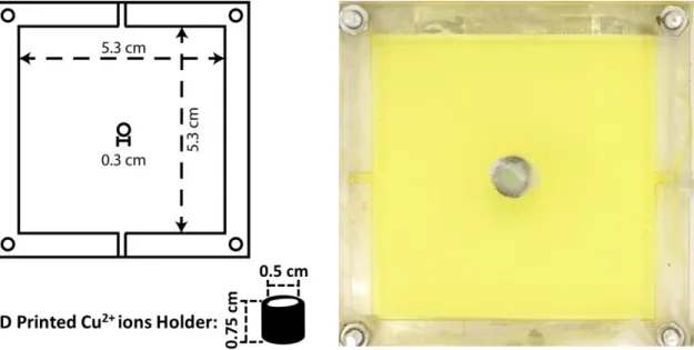
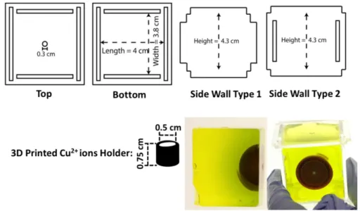
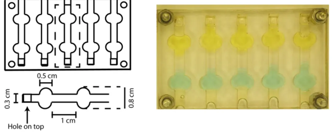
Figure 5: (Left) In our system, outer electrolyte, A, is 1 M copper(II) chloride, and 0.01 M potassium chromate is the inner electrolyte. Over the passage of time, we observe periodic precipitates of copper(II) chromate as dark lines. The diffusion of the outer electrolyte is from left to right in the photos. The time is given in hours. Scale bar is 1 cm. (Right) The hydrogel medium chosen in our experiments is polyacrylamide with bis-acrylamide as the cross-linker. ... 8 Figure 6: (Left) The dimensions of the spacer mold used for 1 D gels. The spacer mold is sandwiched between two plexiglass pieces with the 8 cm x 5.5 cm dimensions, using screws. (Right) the 1D gel samples (yellow) prior to the addition of the outer electrolyte are shown. ... 11 Figure 7: (Left) The dimensions of the mold for 2D gel sheets. The „top‟ side has a hole of the diameter of 0.3 cm in the middle. The 3D printed Cu2+ holder is attached on top of the hole using Superglue. (Right) A 2D gel sheet (yellow) in the mold with the „copper ions holder‟ prior to the addition of the outer electrolyte is shown. Thickness of the gel is 0.2 cm. ... 12 Figure 8: (Top) The dimensions for each of the sides of the cubical box. The pieces are fitted into one another and the edges are sealed from outside using Ecoflex. The 3D printed Cu2+ holder is attached to the top face of the cube. 3D samples with patterns formed inside the cubical box are shown at the bottom right. ... 13 Figure 9: (Left) The dimensions of the mold to prepare a 1 cm x 0.3 x 0.2 cm PAM gel column is shown. The dimensions of each reservoir of electrolytes are 0.5 x 0.8 x 0.2 cm. (Right) Mold with the addition of the copper(II) chloride and potassium chromate reservoirs on each side of 1 cm polyacrylamide gel stripe. ... 14 Figure 10: The experimental setup for controlled temperature experiments. ... 16

vii

Figure 11: The home-built device can keep the temperature constant over time and then ramp the temperature at the desired rate to a certain temperature. Here the first three plots show the temperature is increased from 20 to 50oC at 0.1, 1, and 10oC/min, respectively. The last three graphs show a decrease from 20 to 50oC at 0.1, 1, and 10oC/min, respectively. ... 17 Figure 12: A) The gray value profile (black line) is plotted for the first photo (top, 0 hrs) and the last photo (bottom, 24 hrs) taken during the experiments. The rings are appearing as dips in the gray-value. B) The gray-value plot over the distance in pixels. C) The negative of the gray-value is plotted against distance, i.e., position in Matlab. The rings now appear as peaks and using a built-in functionality of Matlab, i.e., „Findpeak‟, the position of a ring can be obtained. The logarithm of position is plotted against the ring number and the slope gives us 1+p (the spacing coefficient). ... 18 Figure 13: A) The difference between the understanding of RGB and HSB is illustrated. Images are converted from RGB to HSB. B), C), D), The images from the diffusion of copper chloride in PAM (without any inner electrolyte) at different times, 0 hours, 3.5 hours and 10 hours. A specific filter for HUE value of 28 is chosen without any regard to saturation and brightness. Following, a mask is applied with respect to that filter. Finally, the images are converted to a binary image with white representing copper ions, and black referring to PAM (without any inner electrolyte). ... 20 Figure 14: Image processing applied to an SEM image. Particles appear as bright spots in the image. Background subtraction is performed in ImageJ to obtain particles as black dots with white background. Particles (grey colored) are selected per image for size determination. 3 photos are analyzed for each ring and a total of 100 particles is considered for sampling. ... 21 Figure 15: A) Liesegang Patterns formed at 20, 30, 40, 50, and 60oC. PC indicates the point of contact between the polyacrylamide gel surface containing 0.01 M K2CrO4 and 1

M CuCl2 solution. PB indicates the point at which the precipitation of CuCrO4 begins.

Scale bar is 1 cm. B) The variation of spacing coefficient in each of the samples at different temperatures. ... 23

viii

Figure 16: Spatial and time evolution of PB for different temperatures. SPB indicates the time at which PB stabilizes at a certain point. The distance between point of contact (PC) and PB is reducing as the temperature is increased. ... 25 Figure 17: The variance between the time and position of the evolution of the patterns is demonstrated. ... 25 Figure 18: SEM images showing the difference between a depletion zone (no ring) and ring region. The scale bar (yellow line) represents 5 µm. The elemental analysis using EDX shows difference between ring and no ring region, with the presence of Cr peak in the ring region only. ... 26 Figure 19: (A)SEM images of ring 1 and 5 from samples at different temperatures. The histograms in front of the SEM images show the distribution of particle size. The scale bar (yellow line) represents 5 µm. (B) Average particle size in Ring 1 and 5 at different temperatures. ... 28 Figure 20: SEM images of ring 7 and 9 from samples at different temperatures. The histograms in front of the SEM images show the distribution of particle size. The scale bar (yellow line) represents 5 µm. (B) Average particle size in Ring 1 and 5 at different temperatures. ... 29 Figure 21: Diffusion of copper ions in polyacrylamide hydrogel without any inner electrolyte is monitored at different temperatures. The presence of diffusing copper ions are represented in white. A) Diffusion of copper ions at each temperature from 0 to 12 hours with time interval between each frame of 2 hours. B) Comparison of how the diffusion in a constant time interval differs with each temperature. T=0 hours, the first frame, and T= 12 hours, the last frame of the time lapse for each of the temperatures. ... 31

ix

Figure 22: (A) UV-Vis absorption spectra of 0.01, 0.025, 0.05, 0.075, 0.1 and 0.25 mM. of potassium chromate solutions. (B) Calibration plot for determining the concentration of chromate ions, plotted from the data obtained in (A) at 365-370 nm. (C) UV-Vis absorption spectra of samples from copper chromate solutions at different temperatures. See section 2.4 for the details of the experimental procedure. (D) The variance in solubility product as a function of temperature is shown in table. The error bars are calculated from (A) and (B) independent experiments. ... 33 Figure 23: The occurrence of the precipitation band in counter diffusion experiments (see section 2.3 for mold preparation). The concentration of K2CrO4 is varied from 4 mM to

10 mM. K2CrO4 is allowed to diffuse against 1 M CuCl2, at temperatures from 20 to

60oC. Scale bar is 1 cm. ... 34 Figure 24: A) The time at which the fronts meet is denoted as T1, and the time for the precipitation band to appear visually is demonstrated as T2. The time for formation of the single precipitation band is the difference between T2 - T1. Plots B to F indicate the time for the formation of a single precipitation band at different potassium chromate concentrations, from 60 to 20oC, respectively. Plot G shows the links the time for the appearance of the band versus temperature at a particular concentration. ... 36 Figure 25: Pattern forming system with different transition times of temperature decrease. (A)From top to bottom, the samples are kept for 2 hours, 4 hours, 8 hours, 10 hours and 12 hours at 60oC during the LP formation, then transferred to 20oC till the 24th hour. Scale bar is 1 cm. (B) The variation in the spacing coefficient of the patterns for different transition times. (C) The variation in the widths of the patterns. The blue arrow marks the point of transition. ... 38

x

Figure 26: The effect of transition to different temperatures (transitions with different (-ΔT values) at a particular time of transition is shown. (-ΔT indicates the difference in temperature between pre- and post-transition times. (A) The samples are placed at higher temperatures (30, 40, 50, or 60 oC) for 6 hours (pre-transition time) and then cooled down to 20oC. (B) Trend in spacing coefficient with respect to change in temperature: orange indicating higher temperatures, blue indicates 20oC for both A and C. Triangle represents 1+p after transition and square represents 1+p before transition. (C) The samples are placed at 20oC for 12 hours (pre-transition time) and then the sample is heated to higher temperatures (30, 40, 50, or 60oC). ... 40 Figure 27: (A) Ramping down from 50 to 20 degree Celsius at 0.1, 10 and 10oC/min from top to bottom. (B) The spacing coefficient variation with respect to the ring number for each of the ramp rate. (C) The widths of the patterns formed with respect to the ring number. Blue arrow indicating the point of transition and the green arrow represents the pattern formed during the transition period. ... 42 Figure 28: (A) Ramping up from 20 to 50 degree Celsius at 0.1, 10 and 10oC/min from top to bottom. Scale bar is 1 cm. (B) The spacing coefficient variation with respect to the ring number for each of the ramp rate. (C) The widths of the patterns formed with respect to the ring number. Red arrow indicating the point of transition and the green arrow represents the pattern formed during the transition period. ... 43 Figure 29: The variation in the space-time evolution of patterns in samples with difference in ramping rate of temperature change. (Right) Samples are placed at 20oC for 17 hours and then temperature is increased to 50oC at ramp rates of 0.1, 1 and 10oC/min and then temperature is fixated at 50oC till 24th hour of the experiment. (Left) Samples are placed at 50oC for 7 hours and then temperature is decreased to 20oC at ramp rates of 0.1, 1 and 10oC/min and then temperature is fixated at 20oC till 24th hour of the experiment. Space-time plots show the change in pattern evolution over time for different initial conditions and ramps. ... 44

xi

Figure 30: The time lapse beyond the transition point towards heating (left) and cooling (right). The direction of bending observed in patterns is demonstrated to be backwards when the system is heated up and forward when the system is cooled down. The time is displayed in hours: minutes. For heating up (left) transition takes place 17th hour while for cooling down (right) the transition takes place at 7th hour. ... 47 Figure 31: Periodic precipitation patterns are allowed to form in temperature conditions (shown left). Patterns are divided into two subclasses A (Patterns formed at 60oC) and B (Patterns formed at 20oC). The instances where a change in bending of patterns A and B starts is illustrated (right) ... 49 Figure 32: Patterns are formed in a sample with temperature variations from 20 to 60oC. Patterns formed at 20oC are highlighted with blue and patterns formed at 60oC are highlighted with red. The SEM images are for rings 1 to 9 with histograms on their right showing the distribution of particle size. The scale bar (yellow line) represents 5 µm. ... 51 Figure 33: Patterns are formed in a sample with temperature variations from 60 to 20oC. Patterns formed at 20oC are highlighted with blue and patterns formed at 60oC are highlighted with red. The SEM images are for rings 1 to 10 with histograms on their right showing the distribution of particle size. The scale bar (yellow line) represents 5 µm. ... 52 Figure 34: A) Cyclic temperature oscillations between 60 and 20oC encoded within the visual appearance of the patterns in 1 D sample. Initially kept at 60oC for 4 hours and then transferred to 20oC for the next 10 hours. At 14th hour the sample is replaced into the 60oC for 4 hours and then temperature is lowered to 20oC till the 24th hour. B) Cyclic temperature changes in a 2D sample. With the plot illustrating the difference in the time evolution of the patterns in comparison to the spatial distance covered by LPs at two different temperatures. C) Cyclic temperature changes in a 3D sample. A cross-section of 3D patterns (Z-axes). D) The effect of changing the temperature on the spacing coefficient and widths (E) of patterns formed in A) and B). ... 54

1

Chapter 1

1. Introduction:

Nature employs patterns in a sublime and intricate fashion [1]. The synthetic pattern formation has been studied not only to reveal the mechanisms behind patterns occurring in nature but also to employ the patterns in technological applications [2] [3]. An important class of pattern forming systems, known as Liesegang patterns (LPs), was first discovered more than a century ago by R.E. Liesegang [4]. LPs are periodic precipitation patterns resulting from reaction-diffusion [5].The occurrence LPs is not limited to laboratory conditions. They have been reported to be occurring in tree trunks and volcanic rocks [6]. Since their discovery, studies have been carried out to build a universal model for LPs and to understand the experimental conditions for different LP systems. A typical experimental set involves two „electrolytes‟ and a media. An outer electrolyte diffuses into the media, in which inner electrolyte is homogeneously distributed. LPs arise due to the reaction between the two electrolytes coupled with diffusion [7]. Different porous media have been reported to have patterned with LPs [8] [9]. Since most of the reactions chosen for LP formation occur in aqueous media, and for the formation of the LP convection has to be eliminated, hydrogels have thus far been mostly used as a suitable media for LP formation.

There are different models used to describe how LPs occur [10]. All of these models fall in two distinct categories; pre-nucleation models and post-nucleation models. Pre-nucleation explains LPs occurrence as a relaxation to an equilibrium state. It exerts on the fact that diffusive flux coupled with reaction results in a system far-from its equilibrium followed by the occurrence of a precipitation band as the system tends away from this non-equilibrium state. On the other hand, post-nucleation model suggests that due to the reaction between the two electrolytes, sol of the precipitate forms with distribution across

2

the media and LPs start to form later on. The occurrence of the precipitation band is not limited to the area of the colloid formation but the aggregation of larger particles (Ostwald supersaturation).

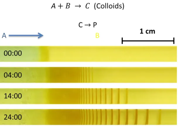
Figure 1: (top) The reaction equation resulting in the formation of LPs. A and B are the counter electrolytes; outer and inner, respectively. C refers to the colloids being produced and the aggregation of the colloids results in the precipitation bands, P (dark bands appearing in the photos below), according to the post-nucleation model. (bottom) The photos of an LP system showing the time evolution of patterns, where A (1 M copper chloride solution) diffuses in to the polyacrylamide hydrogel containing homogeneously distributed B (0.01 M potassium chromate) resulting in the precipitation bands, P, of copper(II) chromate. A is diffusing from left to right in all photos. Scale bar= 1 cm. Time is shown in hours.

Outer electrolyte A reacts with inner electrolyte B and this results in the formation of colloids, C which then nucleate to produce P (figure 1). The precipitation product appears

3

as visually distinct regions in the medium, e.g., in the system shown in Figure 1, they are the dark stripes in the photos of the system. LPs follow a set of mathematical laws, defined as spacing law [11], time law [12], and width law [13] (figure 2). Periodic precipitation bands form a geometric series and in most cases the distance between the patterns is increasing, i.e., an ascending series in terms of the spacing between the bands. For some systems, a descending series has been observed as well [14]. The first is called normal banding, while the latter is referred to as revert (inverse) banding phenomenon. The spacing between consecutive bands is characterized by the spacing law. Similarly, the width of the bands increases from beginning of precipitation to the end (width law). The last empirical law satisfied by Liesegang phenomenon, called as the time law, illustrates that LP formation follows diffusion-controlled kinetics [15].

Figure 2: Mathematical relationships of spacing law, width law and time law with respect to the position of Liesegang patterns are shown. Xn refers to the distance (position) of the

band with respect to the source of outer electrolyte. Xn+1 refers to the position of the next

consecutive band (spacing law). Similarly, Wn refers to the width of the band and Wn+1

refers to the width of the next consecutive band (width law). Time law draws a relationship between the positions (Xn) of the band with respect the time (t) at which

4

1.1.

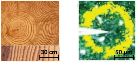
Pattern formation occurs in non-equilibrium systems with the interplay of reaction-diffusion [2]. In these systems, there are chains of complex events and the sum of these complex events form the visual patterns. There is an enormous potential for pattern forming systems to be employed in sensing technologies [16]. Any changes in the physical parameters directly affect these complex events and leave an „impact‟ on the visual sums (patterns). Figure 3 (right) illustrates how dynamic patterns in the form of calcium waves enter retinal cells upon mechanical stimulation [2]. Such examples illustrate that patterns do possess the ability to reveal information about the surroundings. Another classic example would be tree rings [17] (figure 3: left). The morphology of the tree rings reveals information about the seasonal temperature changes in the surroundings and in certain cases, they also reveal the incline growth of the trees. The study of tree ring patterns is known as dendrochronology. It is the science of studying tree-trunk patterns to understand the changes in climatic and atmospheric conditions during the tree growth.

Figure 3: (Left) Cross-section of a tree trunk with distinguishable tree rings. (Right) Ca waves entering a retinal cell upon mechanical stimulation, reproduced from Grzybowski, „Chemistry in motion‟[2].

In our previous study [16], we illustrated how mechanical deformation can be tracked based on the evolution of the periodic precipitates. LPs form in both loaded (deformed)

5

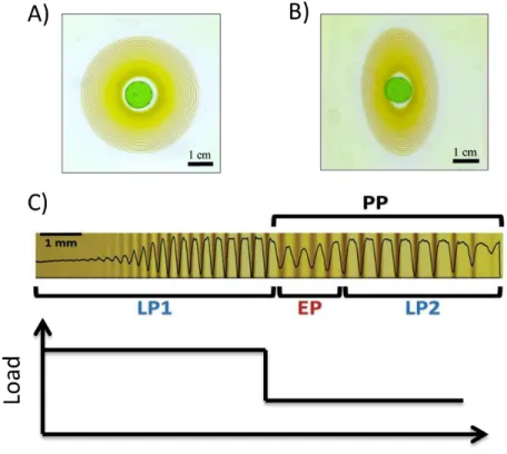
and unloaded (no deformation) samples (figure 4). LPs shown in 4A were formed in the hydrogel undergoing zero percent stretch, while 4B demonstrates how LPs appear in a 40% loaded (stretched) sample after unloading. Furthermore, LPs were also able to signal the instances of the elastic deformation (figure 4C). The occurrence of the equidistant patterns (EP) upon the removal of the load marks the instance of unloading. Upon unloading the sample, there is a change in the flux of outer electrolyte (an increased concentration at that point) leading to production of EPs. This technique was employed to understand not only the extent of deformation, but also the time and duration of the deformation was revealed in the visual appearance of LPs. Henceforth, the relationship between the environment and LPs is definitely optically visible.

Figure 4: A) LPs formed in 2D arrays at 20oC B) LPs formed in elastically deformed 2D array. C) Occurrence of the equidistant patterns (EP) when the load is removed i.e. no elastic deformation. EP bridges the two ascending series that exhibit Liesegang characteristics, LP1 and LP2 [16]. The system comprises of 1 M copper(II) chloride (outer electrolyte), 0.01 M potassium chromate (inner electrolyte) and polyacrylamide gel (media).

6

1.2.

Mechanically[16] probing LPs was the first study that exhibited how change of flux of ions can help achieve control over patterns. Previously, there have been studies related to understanding the effect of electric [18] and magnetic fields [19]. Along with, studies have been focused on understanding the effect of concentration of the electrolytes [20]. Different concentrations of the gels have also been studied as well as of the degree of cross-linking in gels [21] [22]. In this study, we have focused on understanding how patterns occur at different temperatures and whether LPs could visually mark the change of the environmental temperature.

1.3.

Pattern forming chemical systems show astonishing figures and follow beautiful trends when studied at different temperatures [23] [24]. Temperature can be either used for quenching patterns or seeing different shapes [25]. Among all other factors, temperature is the only factor that affects reaction rate, diffusion coefficient and precipitation threshold at once [26]. Temperature has been reported as a factor for increasing the probability of helical patterns in cylindrical gels and alter pattern shape [27]. Earlier studies indicate that temperature affects diffusion coefficient and precipitation threshold [28]. Isemura‟s study revealed that temperature affects number of bands and the width of the depletion zone between the rings. The number of bands decreases and the spacing interval between the bands is reported to increase with temperature, in most cases. However, Popp‟s study showed that the bands were forming closer at higher temperatures [28]. These two contradictory observations are due to the difference in the solubility product‟s dependence on temperature. For instance, Mg(OH)2 [28] is more soluble under

cold conditions while Ag2CO3‟s [28] solubility increases with temperature. Another study

indicated that no trend is observed in the spacing coefficient when experiments are conducted on specific temperatures [29]. However, all these studies are carried out in the temperature range of 0 to 30oC. Han reported LPs at 40oC that had higher spacing between them than at 30oC, but the rings were broken at 40oC [30]. The above-mentioned

7

studies involved Agarose and gelatin as the media of choice; above 45oC agarose gel undergoes phase separation between its components [31] while gelatin melts over 30oC, thus it becomes difficult to form and characterize LPs at temperatures higher than 40oC. It is advised to keep the temperature low and constant to observe periodic precipitation in these gels [32]. However, Antal et al. also suggested that guiding fields, temperature or pH, can result in revert banding, equidistant banding and these guiding fields could be used for pattern control [33]. These characteristic bandings could be achieved by changing the flux of the ions. Nonetheless, no such experimental observation is reported in the literature with changing temperature.

Here we propose a study that quantifies the effect of temperature on Liesegang phenomenon. We show how temperature affects LPs of CuCl2 (outer electrolyte)/K2CrO4

(inner electrolyte) in polyacrylamide gel. Polyacrylamide is a covalently cross-linked, stretchable hydrogel and its glass transition temperature is between 170 and 190oC, depending on the degree of cross-linking [34]. Thus, Polyacrylamide gel acts as a thermally stable media for ambient temperatures (20 to 60oC) considered in this study.

8

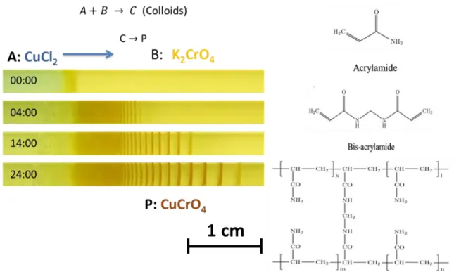
Figure 5: (Left) In our system, outer electrolyte, A, is 1 M copper(II) chloride, and 0.01 M potassium chromate is the inner electrolyte. Over the passage of time, we observe periodic precipitates of copper(II) chromate as dark lines. The diffusion of the outer electrolyte is from left to right in the photos. The time is given in hours. Scale bar is 1 cm. (Right) The hydrogel medium chosen in our experiments is polyacrylamide with bis-acrylamide as the cross-linker.

1.4.

A species diffuses into a media with a linearly spreading velocity. Periodic precipitation patterns occur in the wake of the reaction front [35]. It is logical to assume that faster moving fronts will produce patterns that will be different than patterns produced in the wake of a slower front. Similarly, if a continually flowing front at a certain velocity is disturbed, i.e. either accelerated or slowed down, there should be difference in the patterns in comparison to the patterns that would have formed without the change in velocity. The speed of the front is directly proportional to the temperature of the

9

surrounding as it directly affects the diffusion coefficient of the outer electrolyte. Thus, temperature can be a tool to alter the flow rates of the reaction front.

Upon heating up the system, it is expected that the flux of outer electrolytes will increase and the reaction front will experience a push. This is referred to as a pushed-front. On the other hand, when we cool down the system, the reaction front experiences a halt and hence, a pulled front. Theoretically it is proven that both coherent (with distinguishable trends) and incoherent patterns (chaotic) can result in the wake of pushed or pulled fronts. At this stage, we assume that LPs will demonstrate coherent patterns when temperature of the system is altered. The only difference between a pushed and pulled front is the occurrence of the relaxation time. Patterns immediately start to form in the wake of the pushed front, however, a pulled front system relaxes to a new initial condition and then patterns are observed [36]. With temperature variations, both pushed and pulled fronts could be monitored and pattern formation is to be observed, as the reaction front is accelerated or slowed down.

10

Chapter 2:

2.

Materials and Methods:

2.1.

Acrylamide (AA) (Sigma-Aldrich, 98 % purity), N,N‟-methylene(bis)acrylamide (BIS) (Sigma-Aldrich, 99% purity), potassium peroxydisulfate (KPS) (Sigma-Aldrich, 99 % purity), N,N,N′,N′-tetramethylethylene-diamine (TEMED) (Sigma-Aldrich, 99% purity), potassium chromate (Merck, 99.5 %), copper(II) chloride dihydrate (Merck, 99 % purity), Methanol (Sigma-Aldrich, 99% purity)

Plexiglass and Parafilm® were used without any chemical modification.

2.2.

Molds for 1D, 2D, 3D and counter-diffusion experiments are designed in Adobe Illustrator and made from plexiglass using a laser cutter. 2 mm thick plexiglass sheet is used for all experiments, thus the thickness of the gels in 1D, 2D, and the counter-diffusion experiments is 2 mm as well.

2.2.1. 1D Gels:

Gel strips are prepared by mixing 0.723 grams of acrylamide, 0.003 grams of N, N'-methylenebisacrylamide (BIS), 0.01 g of potassium persulfate, and 0.01 g of potassium chromate as the inner electrolyte. A total of 4.8 ml of water is added to dissolve all the ingredients. The solution is ultrasonicated for 2 minutes. 10 microliters of tetramethylethylenediamine (TEMED), a free-radical initiator, is added to the gel

11

solution. The gel solution is then transferred to the mold and the top of the mold is closed by a piece of plexiglass. After approximately, 24 hours, 1 M CuCl2 is introduced to the

top of the gel. A small drop of oil is added on top of CuCl2 solution inside the mold to

reduce the evaporation of CuCl2 solution. The gel is then placed horizontally, onto the

home-built device (see below), which is adjusted to the desired temperature.

Figure 6: (Left) The dimensions of the spacer mold used for 1 D gels. The spacer mold is sandwiched between two plexiglass pieces with the 8 cm x 5.5 cm dimensions, using screws. (Right) the 1D gel samples (yellow) prior to the addition of the outer electrolyte are shown.

12

2.2.2. 2D gels:

1.446 grams of acrylamide, 0.006 grams of N, N'-methylenebisacrylamide, 0.02 g of potassium persulfate, and 0.02 g of potassium chromate as the inner electrolyte are dissolved in a total of 9.6 ml of water . The solution is ultrasonicated for 5 minutes. 10 microliters of tetramethylethylenediamine (TEMED), a free-radical initiator, is added to the gel solution. The gel solution is then transferred to the mold through the „copper ions holder‟. And the top of the holder is closed by a piece of Parafilm. After approximately, 24 hours, 1 M CuCl2 is introduced to the top of the gel through the „copper ions holder‟.

A small drop of oil is added on top of CuCl2 solution inside the mold to reduce the

evaporation of CuCl2. The gel is then placed horizontally, onto the home-built device (see

below), which is adjusted to the desired temperature.

Figure 7: (Left) The dimensions of the mold for 2D gel sheets. The „top‟ side has a hole of the diameter of 0.3 cm in the middle. The 3D printed Cu2+ holder is attached on top of the hole using Superglue. (Right) A 2D gel sheet (yellow) in the mold with the „copper ions holder‟ prior to the addition of the outer electrolyte is shown. Thickness of the gel is 0.2 cm.

13

2.2.3. 3D gels:

3D blocks of gels are prepared in a plexiglass box (figure 8). The box is assembled and the outer edges are sealed with Ecoflex, to prevent any leakage. For a 3D block of PAM hydrogel, the precursor solution was scaled to 7 times of a 2D gel. 10.112 grams of acrylamide, 0.042 grams of N, N'-methylenebisacrylamide, 0.14 g of potassium persulfate, and 0.14 g of potassium chromate as an inner electrolyte. A total of 67.2 ml of water is added to dissolve all the ingredients. The solution is ultrasonicated for 5 minutes. 70 microliters of tetramethylethylenediamine (TEMED), a free-radical initiator, is added to the gel solution. The gel solution is then transferred to the plexiglass box through the „copper ions holder‟ at the top. The top of the holder is closed by parafilm to reduce evaporation. After approximately, 24 hours, 1 M CuCl2 is introduced to the top of the gel

through the copper ions holder. A small drop of oil is added on top of CuCl2 solution

inside the mold to reduce the evaporation of CuCl2. The 3D block of gel is then placed in

an oil-bath set at the desired temperature.

Figure 8: (Top) The dimensions for each of the sides of the cubical box. The pieces are fitted into one another and the edges are sealed from outside using Ecoflex. The 3D printed Cu2+ holder is attached to the top face of the cube. 3D samples with patterns formed inside the cubical box are shown at the bottom right.

14

2.3.

A mold is designed to be capable of holding a 1 cm column of polyacrylamide hydrogel without any inner electrolyte. The molds are designed similarly to the 1D gel, i.e., a spacer mold of height 0.2 cm is sandwiched between two plexiglass pieces of the same dimensions. The spacer‟s one end is closed, while the other end has an open mouth. The plexiglass piece at the top has a cube-like opening of dimensions 0.3 cm x 0.3 cm into the spacer. 0.73 grams of acrylamide, 0.0015 grams of N, N‟-methylenebisacrylamide, 0.01 g of potassium persulfate are weighed in a beaker. The crosslinker concentration is reduced as there is no potassium chromate inside the hydrogel. A total of 4.8 ml of water is added to dissolve all the ingredients. The solution is ultrasonicated for 2 minutes. 5 microliters of tetramethylethylenediamine (TEMED), a free-radical initiator, is added to the gel solution. The gel solution is then transferred to the plexiglass mold from the open end. The solution is injected carefully to achieve a 1 cm polyacrylamide gel stripe. After approximately, 24 hours, 1 M CuCl2 is introduced through the open end of the mold. The

desired concentration of potassium chromate is inserted through the cube-like opening on the top plexiglas piece. A small drop of oil is added on top of CuCl2 and K2CrO4 solution

inside the mold to reduce the evaporation of the liquid solutions.

Figure 9: (Left) The dimensions of the mold to prepare a 1 cm x 0.3 x 0.2 cm PAM gel column is shown. The dimensions of each reservoir of electrolytes are 0.5 x 0.8 x 0.2 cm. (Right) Mold with the addition of the copper(II) chloride and potassium chromate reservoirs on each side of 1 cm polyacrylamide gel stripe.

15

2.4.

water

Copper chromate is synthesized by mixing copper(II) chloride solution with potassium chromate. 6.7 grams of copper(II) chloride and 9.7 grams of potassium chromate are dissolved separately in 250 ml of water each. Both solutions are ultrasonicated till the point a complete dissolution has occurred. Copper(II) chloride solution is added slowly to the potassium chromate solution. The reaction mixture is stirred using a teflon coated magnetic stirring bar for the next 12 hours. Copper(II) chromate is filtered out from the reaction mixture using vacuum filtration. The precipitate is washed with 200 ml of water in 8 subsequent washes. The precipitate is then washed with 200 ml of methanol in 8 subsequent washes. Copper(II) chromate is transferred to a mortar and crushed down fine powder. The precipitates are dried overnight under vacuum at room temperature.

25 mg of Copper(II) chromate is weighed in a glass vial and 2 ml of water is added to it. A total of five samples are prepared for each temperature. The vials are transferred to an oil bath set at desired temperature. The mixtures are stirred using PTF coated magnetic stirring bars for at least 12 hours. After 12 hours, the solution is transferred to a syringe (pre-heated at a higher temperature), and filtered using a syringe filter (pre-heated at higher temperature). 0.5 ml of the filtrate is diluted to 10 ml solution with water, to prevent any dissolution. 2 ml of this solution is further diluted to 10 ml with water. The solutions are then analyzed with UV-Vis spectroscopy between 365 - 370 nm to obtain the concentration of chromate ions. A calibration plot for UV-Vis spectroscopy is obtained from 0.01, 0.025, 0.05, 0.075, 0.1 and 0.25 mM solutions of potassium chromate prepared by appropriate dilutions. The concentration of chromate ions is determined using Beer Lambert law.

16

2.5.

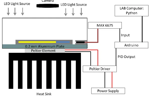
Figure 10: The experimental setup for controlled temperature experiments.

The temperature is controlled by a home-built setup using a Peltier element. Peltier element works under the principles of thermoelectric cooling and the effect is known as the Peltier effect. The Peltier element employed in our device is 12706. TEC1-12706 has a maximum current rating of 6.4 Amps, a maximum voltage rating of 14.4 volts. The two sides of the Peltier element are coated with locally obtained, silicon-based thermal paste and is sandwiched between a heat sink and a 2 mm thick aluminum plate. Thermocouple is sandwiched between two plexiglass plates in a similar fashion as hydrogels. We use a K-type thermocouple with temperature ratings between -20 to 80-degree Celsius and interface it with an Arduino Nano, using MAX-6675 which digitalizes the signal from the thermocouple. MAX-6675 provides a 12-bit resolution to the temperature data, i.e. 0.25 degree-celsius. Arduino Nano is in interface with Spyder Python in a desktop computer. Data from MAX-6675 is the input to the PID loop. PID output drives the Peltier Element using a Peltier Driver through Arduino Nano. Peltier

17

Driver used in our setup is a half-bridge, BTS 7960B DC Motor driver. The BTS 7960B DC Motor driver has a maximum current rating of 40 Amps and working voltages range from 5.5 to 27.5 Volts.

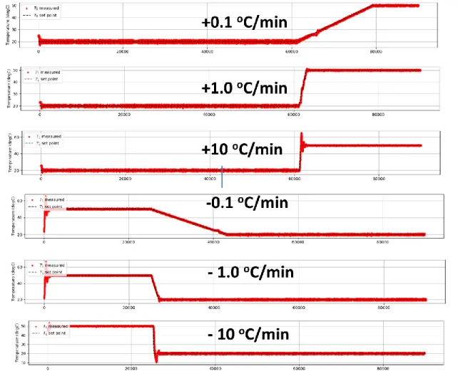
Figure 11: The home-built device can keep the temperature constant over time and then ramp the temperature at the desired rate to a certain temperature. Here the first three plots show the temperature is increased from 20 to 50oC at 0.1, 1, and 10oC/min, respectively. The last three graphs show a decrease from 20 to 50oC at 0.1, 1, and 10oC/min, respectively.

18

2.6.

2.6.1. Determination of spacing coefficient

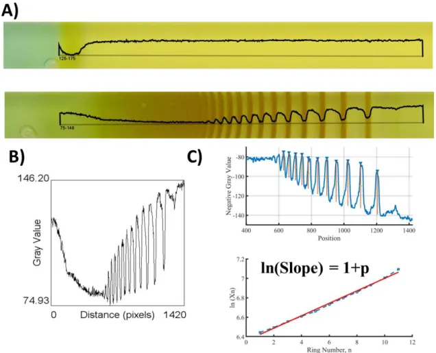
Figure 12: A) The gray value profile (black line) is plotted for the first photo (top, 0 hrs) and the last photo (bottom, 24 hrs) taken during the experiments. The rings are appearing as dips in the gray-value. B) The gray-value plot over the distance in pixels. C) The negative of the gray-value is plotted against distance, i.e., position in Matlab. The rings now appear as peaks and using a built-in functionality of Matlab, i.e., „Findpeak‟, the position of a ring can be obtained. The logarithm of position is plotted against the ring number and the slope gives us 1+p (the spacing coefficient).

Liesegang Rings are quantified by extracting the information about the position of the rings using ImageJ software. Image of LPs is loaded to ImageJ and the „gray-value‟ of a

19

single-line selection is plotted. Gray-Value refers to a combination of the three-color components of the image i.e. red, green, and blue. The formula used for quantifying the gray value is 0.299red + 0.587green + 0.114blue. Gray value plot shows the rings as the sharp dips in the gray value. Following that, the raw data of the gray value vs pixel position plot is loaded into Matlab. The negative of the gray value is plotted so that rings appear as peaks. Position, width, and prominence are determined by a built-in functionality of Matlab i.e. „Findpeaks‟. The position of the ring (Xn) is determined for

each peak, by finding the distance at which local maxima in negative gray value occurred. „Prominence‟ is the maximum gray value. Width is determined by full-width at half maxima. The spacing law is determined by taking a logarithm of positions then plotting the graph of ln(Xn) versus the number of rings. The slope of this plot is the spacing coefficient.

2.6.2. Determining Time Law

The time law is determined by loading the stack of images into ImageJ. Each frame in the image stack represents an image taken at a 5 min interval. The point of contact (PC) between the gel and the outer electrolyte is chosen as a reference point for all the images. The position of the rings is determined by streching the line from PC to the middle of the ring. The time is decided as the point where ring starts to form. A plot is plotted regarding the relationship between the postion of the ring and the square root of time.

2.6.3. Image processing for tracking diffusion of Copper ions

The diffusion of copper ions is qualitatively tracked by converting the images from RGB to HSB stack in OpenCV (figure 13). Following that, a mask is applied for HSV values of [28, 0, 0]. HUE values above 28 are masked by the color filter. The resulting image is converted to a binary image of 0 and 1, where 0 illustrates HUE values below 28 and 1 all the HUE values above 28. In the final image, copper ions are represented as white, and black refers to the polyacrylamide gel matrix without any inner electrolyte. In this way, the signal to noise ratio for tracking the diffusion of copper ions is improved.

20

Figure 13: A) The difference between the understanding of RGB and HSB is illustrated. Images are converted from RGB to HSB. B), C), D), The images from the diffusion of copper chloride in PAM (without any inner electrolyte) at different times, 0 hours, 3.5 hours and 10 hours. A specific filter for HUE value of 28 is chosen without any regard to saturation and brightness. Following, a mask is applied with respect to that filter. Finally, the images are converted to a binary image with white representing copper ions, and black referring to PAM (without any inner electrolyte).

21

2.7.

The size distribution of patterns is analyzed using SEM. Hydrogel sample with freshly formed periodic precipitates at a desired temperature is placed horizontally in a glass flask. The flask is vacuumed and transferred to liquid nitrogen bath for the next 30 minutes. Frozen hydrogels are placed on a stand pre-cooled with liquid nitrogen. The samples are cut in half using a steel blade and transferred to a petri dish, with the freshly cut side on top. Petri dish is covered with aluminum foil and then placed under vacuum at room temperature for 24 hours.

Scanning Electron Microscopy (SEM) and Energy Dispersive X-Ray (EDX) Analyses.

The surface morphology of gel samples were imaged and analyzed with a Quanta 200F model SEM with an accelerating voltage of 10 kV. Samples were coated with Au-Pd. The size of the particles was determined using digital image analysis ImageJ software (figure 14).

Figure 14: Image processing applied to an SEM image. Particles appear as bright spots in the image. Background subtraction is performed in ImageJ to obtain particles as black dots with white background. Particles (grey colored) are selected per image for size determination. 3 photos are analyzed for each ring and a total of 100 particles is considered for sampling.

22

Chapter 3

3.

Results and Discussion:

3.1.

In our system, Cu2+ ions diffuse into the gel from one side (1D) and react with CrO4

2-ions homogeneously distributed inside the gel.

A (Colloids) C P

In the Liesegang phenomenon, temperature affects the diffusion of Cu2+ ions, the rate of colloid formation, and stability of the colloids to form periodic precipitates. Therefore, pattern evolution is expected to be visually distinctive concerning the different temperatures. LPs are allowed to form, at a constant temperature, for 24 hours (Figure 15A). Periodic patterns are observed in the range from 20 to 60oC. With every 10oC increments in increasing temperature, wider depletion zones between periodic precipitates occur. The position of the last band is further in the spatial coordinate for every 10oC increment. Figure 15B also illustrates how the relationship between point of contact (PC) and precipitation begins (PB) varies with increments in temperatures. The distance between PC and PB decreases at a higher temperature as compared to lower temperatures.

23

Figure 15: A) Liesegang Patterns formed at 20, 30, 40, 50, and 60oC. PC indicates the point of contact between the polyacrylamide gel surface containing 0.01 M K2CrO4 and 1

M CuCl2 solution. PB indicates the point at which the precipitation of CuCrO4 begins.

Scale bar is 1 cm. B) The variation of spacing coefficient in each of the samples at different temperatures.

Furthermore, the visually distinctive features like wider depletion zones and the position of the last ring are mathematically quantified by the spacing coefficient. Spacing law is one of the benchmark characterizations of LPs.

The spacing law is:

where Xn and Xn +1 are the positions of the nth and (n + 1) the bands measured from the

gel surface, respectively, and p is the so-called spacing coefficient. PC is chosen as a reference point for all the samples. Figure 15B illustrates how the spacing coefficient demonstrates a direct relationship with temperature.

Figure 16 shows the shifts in distance between PC and PB over time. At the start of diffusion, continuous precipitation is observed. This precipitation zone re-dissolves and seemingly, the precipitation front propagates. For instance, at 20oC dissolution occurs in

24

various instances until 12 hours, resulting in a higher distance between PC and PB. At 30 and 40oC, stabilized precipitation begins (SPB) after 6 hours, i.e. no significant dissolution occurs later on. Following the trend, SPB occurs after 2 hours into the reaction-diffusion processes at 50 and 60oC. Thus, the distance between PC and PB evolves and PB stabilizes both closest to PC and earlier in time coordinate at 60oC compared to lower temperatures. This dissolution of CuCrO4 can be related to several

factors. And such dissolution is not unique to this system. Similar behavior occurs in the Co(OH)2 [37] system in which periodic precipitates dissolute. This observation occurs as

a result of complexation reactions. Since the dissolution is limited to the beginning of continuous precipitation, our results may find their explanation in the dissolution of small colloids. For the precipitates to be stable in the gel media, they need to aggregate into bigger particles. Colloid diffusion is limited in gel media as a result smaller colloids dissolute and re-precipitates to form bigger aggregates. Thus, the occurrence of earlier SPB and lower distance between PC and PB at higher temperatures could lead us to conclude one of the following: 1) aggregation of CuCrO4 colloids could be favored by

higher temperatures (higher kbT i.e. an increased energy possessed by the particles for

aggregation at higher temperatures), 2) naturally, the particle size of CuCrO4 colloids

could increase with temperature [38]. Each of these factors is interrelated since precipitation threshold is a measure of the number of colloids and their sizes at a specific position in the media. The exact conclusion is far from reach, however, visually distinctive features (PC, PB, and SPB) point towards an essential interplay between different factors.

25

Figure 16: Spatial and time evolution of PB for different temperatures. SPB indicates the time at which PB stabilizes at a certain point. The distance between point of contact (PC) and PB is reducing as the temperature is increased.

The space-time relationship is demonstrated in figure 17. The slope of the graph increases according to the increments in temperature. LPs form further in the spatial coordinate at a faster rate at higher temperatures.

Figure 17: The variance between the time and position of the evolution of the patterns is demonstrated.

26

3.2.

The occurrence of late SPB at lower temperatures (figure 16) was reasoned by the hypothesis of very small particle size in the beginning of the reaction-diffusion. Here, we demonstrate the effect of temperature on the particle size in Liesegang phenomenon. LPs appear as bands of concurrent periodic precipitates; these bands result from the aggregation of small particles. Figure 18 illustrates the difference between a depletion zone i.e. no ring region and ring region at resolution of 5 micro meters. The ring region of the gel consists of particles as bright spots and EDX spectrum confirms the presence of copper(II) chromate particles by the occurrence of chromium peak in ring region only.

Figure 18: SEM images showing the difference between a depletion zone (no ring) and ring region. The scale bar (yellow line) represents 5 µm. The elemental analysis using EDX shows difference between ring and no ring region, with the presence of Cr peak in the ring region only.

27

Samples from each constant temperature experiments were analyzed under SEM for determination of particle sizes. Here we show the relationship between temperature and particle size in Ring 1, 5, 7 and 9 (the Last Band). In figure 19A, SEM images of ring 1 and 5 from constant temperature experiments are shown, along with, the histograms showing the distribution of particle size. Figure 20A compares the SEM images of ring 7 and 9, forming at different temperatures, along with, the histograms showing the distribution of particle sizes. The general trend observed is an increase in the particle size along the ring number as reported in literature [39]. However, the particle size for a simultaneous ring varies a lot with temperature. Particles at ring 1 from the sample kept at 60oC, has considerably higher size then particles observed for ring 1 from sample kept at 20oC. Similarly, every 10oC increment in temperature increases the particle size for the simultaneous ring. The particle size and distribution at different temperatures are visually very distinct from each other at ring 1, 5, 7 and 9. The visual observation is further strengthened from the particle size histograms.

28

Figure 19: (A)SEM images of ring 1 and 5 from samples at different temperatures. The histograms in front of the SEM images show the distribution of particle size. The scale bar (yellow line) represents 5 µm. (B) Average particle size in Ring 1 and 5 at different temperatures.

29

Figure 20: SEM images of ring 7 and 9 from samples at different temperatures. The histograms in front of the SEM images show the distribution of particle size. The scale bar (yellow line) represents 5 µm. (B) Average particle size in Ring 7 and 9 at different temperatures.

30

3.3.

Diffusion Coefficient (kd) of copper ions in polyacrylamide gel, Precipitation Threshold

(i.e. the number/ concentration of colloids required for a band to occur) and Reaction Coefficient (kp) of the reaction between copper ions and chromate ions are independently

affected by temperature. Precipitation threshold is directly affected by the solubility of the copper(II) chromate, therefore, the solubility product (Ksp) of copper(II) chromate at

different temperatures is to be determined. For a reaction-diffusion system, kd,kp, and Ksp

are interlinked with each other, thus in order to quantify effect of temperature on LPs each of these need to be treated independently in most similar fashion to our system.

3.3.1. Understanding the Diffusion

The diffusion coefficient in porous media like hydrogels is related to the porosity of the media. And to discover the relationship between diffusion coefficient and temperature, the link between the porosity of polyacrylamide hydrogel and temperature needs to be uncovered. Since copper ions can complex with the polyacrylamide matrix, the ability of copper ions to diffuse can also vary with temperature. The complexing ability of copper ions might also alter the porosity of the hydrogel. This claim finds its basis in the work of Korevaar et al, where they demonstrate that diffusing fronts can result in the appearance of a physical wave [40]. Therefore, we understand this problem by preparing polyacrylamide hydrogels, without any inner electrolyte (Potassium Chromate) and introduce a reservoir of copper ions from one end (1D). The diffusion of copper ions is monitored for 12 hours at a constant temperature.

Figure 21 shows how the copper front diffuses inside the hydrogels at different temperatures. Color filtering is applied (see Section 2.7.3 for further details of image processing) to understand the position of the copper front inside the hydrogel more precisely. As illustrated in figure 21, the Cu2+ front moves faster and further at higher temperatures.

31

Figure 21: Diffusion of copper ions in polyacrylamide hydrogel without any inner electrolyte is monitored at different temperatures. The presence of diffusing copper ions are represented in white. A) Diffusion of copper ions at each temperature from 0 to 12 hours with time interval between each frame of 2 hours. B) Comparison of how the diffusion in a constant time interval differs with each temperature. T=0 hours, the first frame, and T= 12 hours, the last frame of the time lapse for each of the temperatures.

3.3.2. Understanding the precipitation threshold

Conventional Liesegang phenomenon is observed for ions producing sparingly soluble salts in aqueous media. Periodic bands of the salt arise inside hydrogels when colloids aggregate to form bigger particles. This process occurs when the concentration of colloids at a certain point (band location) surpasses the precipitation threshold. Solubility product plays an important role in determination of a precipitation threshold for the system. The indirect relationship between the precipitation threshold and the solubility product indicates that for salts with high Ksp will require a higher concentration or bigger

size of colloids to aggregate and vice versa. This relationship also alters the spacing between the bands. As a reaction-diffusion system propagates, the concentration of inner electrolyte depletes behind and in front of the band. For the next band to occur the outer electrolyte diffuses further and the concentration of colloids rise to form the next band,

32

however this time at a different place in hydrogel [37]. Now if we have two sparingly soluble salts, one with the Ksp value higher than the other. The creation of the second

band will require higher concentration of the colloids for the salt with higher Ksp. Thus,

the colloids will be forming and dissolving to form bigger particles and aggregate further in the spatial coordinate to form the next consecutive band. As a result, spacing between patterns formed for the salt with higher Ksp will be greater in comparison to the system

having lower Ksp. Solubility product also affects the particle size. For salts with lower Ksp

values, the supersaturation is high, and colloids surpass precipitation threshold easily. Hence, dissolution of colloids to form bigger aggregates occurs at a lower frequency than for the salt with higher Ksp. Thus, solubility product holds an essential place in the

equation, from existence of bands, to the spacing between them to the size of the aggregates.

In our system, LPs of copper(II) chromate are forming at different temperatures and solubility product is varying with temperature. In order to determine the solubility product at the different temperatures used in the experiments, copper(II) chromate is separately formed from its aqueous ions and the solubility product is determined in a similar fashion as Coetzee et al. reported [41]. (The experimental details of this procedure are given in Section 2.4). Here in figure 22 we illustrate how the solubility product changes with temperature. The dissolution of copper(II) chromate is assumed to occur as,

CuCrO4 (s) ⇌ Cu2+ (aq) + CrO42- (aq)

Solubility product of copper(II) chromate rises with the temperature of the system (figure 22D). Maximum absorption between 365-370 nm [42] is used for the calculation of concentration of chromate ions using the molar absorption coefficient, 4.048 L⋅mol−1⋅cm−1 (figure 22B). Our results about the increase in the spacing between the rings (figure 14), occurrence of earlier stabilized precipitation (figure 16) and an increase in the size of the particles (figure 19 and 20) can be explained by dramatic increase in the values of the solubility product as the temperature of the system rises.

33

Figure 22: (A) UV-Vis absorption spectra of 0.01, 0.025, 0.05, 0.075, 0.1 and 0.25 mM. of potassium chromate solutions. (B) Calibration plot for determining the concentration of chromate ions, plotted from the data obtained in (A) at 365-370 nm. (C) UV-Vis absorption spectra of samples from copper chromate solutions at different temperatures. See section 2.4 for the details of the experimental procedure. (D) The variance in solubility product as a function of temperature is shown in table. The error bars are calculated from (A) and (B) independent experiments.

34

3.3.3. Understanding the Reaction Coefficient

Figure 23: The occurrence of the precipitation band in counter diffusion experiments (see section 2.3 for mold preparation). The concentration of K2CrO4 is varied from 4 mM to

10 mM. K2CrO4 is allowed to diffuse against 1 M CuCl2, at temperatures from 20 to

35

Here in figure 23, we prepare a 1 cm polyacrylamide gel matrix without any inner electrolyte (See Section 2.3 for details on experimental preparation), and introduce a reservoir of Cu2+ ions from one end and another reservoir of potassium chromate form the other end. The two reactants are allowed to simultaneously diffuse into the hydrogels and finally react with each other to produce a precipitation band. This is followed by the formation of the revert periodic precipitation patterns. The concentration of potassium chromate is varied between 4 mM and 10 mM and the concentration of copper chloride is kept constant at 1 M (See Section 2.3 for experimental details).

The trend indicates that with increasing temperature, the precipitation threshold decreases (see section 3.3.2 for discussion). The results in figure 23 do not demonstrate a decrease in the solubility product with increasing temperature. The occurrences of a precipitation band for lower concentrations of chromate at higher temperatures can be due to aggregation of large particles (as particle size increases with the temperature of the system, see figure 19 and 20).

The feature extracted from the counter diffusion experiment is the time it takes for the band to appear after the two fronts have met (figure 24A). Figure 24B to F illustrates the time required for the bands to appear for different concentrations of potassium chromate. The results indicate for each temperature value, less time is required for a band to appear at higher concentrations. The relationship between time for the formation of the precipitation band and the temperature for a particular concentration is plotted in figure G. These results indicate that from the time the fronts meet to the point a precipitation band is formed; with increasing temperature, all processes occur at an increased rate; 1) the rate of formation of colloids, their dissolution and reformation, 2) surpassing the precipitation threshold, 3) aggregation of colloids into the bands. Therefore, we can conclude that the reaction rate is being positively affected by the increase in temperature.