1
Mediation of Foreign Direct Investment and Agriculture towards Ecological
footprint: A shift from single perspective to a more inclusive perspective for
India
Edmund Ntom UDEMBA
Faculty of Economics Administrative and Social sciences, Istanbul Gelisim University, Istanbul, Turkey Correspondence: Email: [email protected];
[email protected]; [email protected].
Tel: +905357808713
WhatsApp: +2347039678122; +905357808713
Funding
The author hereby declares that there is no form of funding received for this study.
Compliance with Ethical Standards
The author wishes to disclose here that there are no potential conflicts of interest at any level of this study.
Abstract
According to Carbon Brief Profile report (2019), India has been identified as the world 3rd largest emitter of greenhouse gases (GHG’s) after China and the US. Following the Paris agreement and India pledge as among the stakeholders at the global climate talks, and how speed the India ratified the Paris Agreement within a year on the 2nd of October, 2016, it is essential to investigate the country’s (India) commitment in reducing its emission towards enhancing a positive environmental performance. Both structural breaks, linear Autoregressive Distributed Lag (ARDL) and nonlinear Autoregressive Distributed Lag (NARDL) were selected simultaneously for this study but at a later stage after bound cointegration estimation, the NARDL was dropped because of its inability to sustain the claim of cointegration in the analysis. The rest of the analyses were based on liner ARDL model (short-run and long-run) with diagnostic tests, Granger causality estimation. Ecological Footprint (EFP) was chosen as an indicator to environment because of its richness in measuring the environmental performance. The linear(ARDL) output affirms a positive and significant links amongst ecological footprint and agriculture, energy use and population with a negative link between ecological footprint (EFP) and foreign direct investment (FDI). The granger causality test indicates one-way transmission passing from agriculture, foreign direct investment, energy use and population to ecological footprint. Also, one-way transmission was
2
found passing to economic growth (GDP) from foreign direct investment (FDI), and feedback transmission was found between FDI and energy use. This finding has implication to both economic and environmental performance, hence the policy framework should be targeting the enhancement of economy via foreign direct investment and agriculture with a focus on the energy use and environmental performance
Keywords: Ecological footprint; FDI; agricultural sector; energy use; economic growth, ARDL-
NARDL; India
JEL Codes: C32, C33, Q43, Q58
1. Introduction.
The recent awareness on the climate change leading to global warming is currently a universal phenomenon and contemporary issue that demands urgent attention from all works of life and all stakeholders, including governments (international, national and local), the private sectors, civil society, local authorities and other international organizations for solution. Following the upsurge of the global warming, there has been adoption and urgent consideration of Paris Agreement as a major force to abate the speedy rise of global warming. A task is presented before both the developed and developing countries to limit the global average climate condition to well below 2 0C and to bring it to a minimal of 1.5 0C and above pre-industrial levels. The climate change is mostly triggered by the dilapidated environment that is most affected by the ecological footprint. The Ecological Footprint summed up all the human activities on Earth that has to do with geographical and biological harnessing of space (Galli, A, 2015). These activities are found in the areas of excavation of natural resources (mining and oil exploration), economic activities, agricultural activities, construction, deforestation, urban infrastructure and transportation. As put by Ulucak and Lin, (2017), ecological footprints measures accommodate diverse stocks such as soil, forestry, exploration of natural resources (mining and oil stocks)
Exploration and the usage of some natural resources such as oil and gas constitute part of the ecological footprint. This is evident in the case of oil spillage within the geographical setting or location of mining of these resources. Most times the spillage is hazardous both to the aquatic life and farm lands which will eventually lead to the death of inhabited animals and fishes and turn them into poisonous sea foods for humans and renders the farm lands infertile. The agricultural practice in some countries including India constitute part of the ecological footprint which eventually lead to unhealthy environment. Land reclaiming for farming purposes which is done via deforestation often leads to exposing of the environment to excessive heat because of inadequate plants and trees to aid in reducing excessive carbon dioxide, and the end result is global warming. Inclusive in agricultural practice in such places like India is the activities of herders and their cows both on land and the water bodies. Most times, the animals are agents of environmental degradation via polluting of the water bodies and the surroundings with methane which is part of the constituents of the greenhouse gas (GHG). The inorganic manures or chemicals such as fertilizers used in farming equally add to the climate change via the release of nitrogen oxide. Survey from Carbon Brief Profile (2019) revealed that agriculture and farming constitute 0.16 percent of Indian ecological footprint (EFP). The result also indicates that pollutants from farming
3
amounts to about 30% of the world in total and that farming is among the major emitters of ecological footprint and emissions.
The economic activities by human agents such manufacturing and production which form part of investment for foreign investors in form of foreign direct investments (FDI) also contribute to the climate change. This involves the usage of heavy duty machines and factory machines which are powered by excessive non-renewable energy consumption which in turn emits carbon dioxide and this emission is considered part of ecological footprint. Though, some studies have found that economic activities in form of FDI is a two-fold agent in impacting the environment. Some are of opinion that it addresses the environmental issue favorably such as investments in clean technologies and in renewable energy which is more environmental-friendly and contributes in addressing the issue of ecological footprint (Udemba et al. 2019; Zhang 2011; Katircioglu and Taspinar 2017), while others are in contrast to this. They argue that FDI encourages the use of heavy duty and excessive energy consumption machines which contributes in expanding the business activities which will promote the acquisition of new plants and machines thereby increase carbon emissions settlements in the environment and impact negatively to the environment (Zhang, W.B., 2018; Danish et al. 2018; Sarkodie and Strezov, 2019; Udemba E.N, 2019). The trade-off between the sustainability of economic momentum in terms of growth and development and the environmental security has become a challenge to the policy makers and this has constituted a major concern to advocates of the environment. The increasing population of many countries including India amounts to serious pressure on the demand and consumption of the natural resources and this is becoming a global challenge. From this perspective, the ecological footprint is described as the extent of a geographical area of organically useful earth and water occupied by a group of people (population), or action needed to yield all the resources it consumes (Global Footprint Network, 2018). The more the increase on the population the more the increase on the consumption of natural resources and the more the increase on the pollution and dilapidation of the environment. Bagliani et al. (2008); Wang et al. (2011); Al-Mulali et al. (2015) and Uddin et al. (2017) suggest that ecological footprint measure the consumption of the natural resources and a reliable parameter for environmental damage.
The emergency and the need to curb the rate of the global warming and the need to proffer solutions to the environmental problems has paved way for many literature emerging from all works of life including the energy and environmental economist. Though, most of the literature have really dealt and almost exhausted the research with a target on C02 emissions as an indicator to measure environmental dilapidation with less focus on the angle of ecological footprint. Most time the reason associated with this is the unavailability of data and its correlation with the greenhouse effect. Aside the C02 emissions, other researchers have adopted other single ecological indicators in studying the impact of environmental quality towards the climate change. However, it is irrational to focus only on one single indicator among the many indicators that make up the ecological footprint when researching on environmental quality. For this reason, (Rees, 1992; Wackernagel, 1994 and Rees and Wackernagel, 1998) modelled ecological footprint as a comprehensive proxy for environmental degradation. Other scholars have utilized foreign direct investment and ecological footprint to ascertain the environmental state with varied results. Most of the studies adopt panel study instead of single country’s analysis (Ali et al., 2020; Destek and
4
Okumus 2019; Majeed and Mazhar 2019; Baloch et al., 2019); Liu and Kim (2018). These studies differ from our study on the areas of focus and their methodology. This present work is strictly a single country’s study with India as a focus. Most times, panel work lacks the power to give in-depth analysis of the sampled countries because heterogeneous nature of the merged or pooled countries. India is an open economy with features that are pollution incline such as population, economy is mostly dependent on agriculture and FDI which place the country in a strategic position for emission involvement. According to Ulucak and Lin, (2017) this model is encompassing and comprises dilapidation in multiple factors such as soil, forestry, exploration of natural resources (mining and oil stocks). The ecological footprint comprises of the sum of six components namely, carbon footprints, built-up land, cropland, grazing land, forest land and fishing grounds. Since the ecological footprint considers several resources stocks, a research based on the ecological footprint will be more effective in considering the environmental quality and modelling of policy measures in sustainability of the economic activities and controlling of the environmental decadence.
It is on this premises that the researcher chose to study the environmental performance of India with the application of a more comprehensive indicator of ecological footprint and the selected variables which are relevant with the uniqueness of the country (India). The fundamental uniqueness of this paper is based on the combination of different empirical techniques and utilization of the ecological footprint to measure the environmental performance of Indian economy. The empirical analyses of this work are not just based on a single analysis but a combination and comparison of different techniques (ARDL-bound test and Asymmetry-NARDL with the support of causality analyses) to give an unbiased and a robust finding that will aid in policy framing towards sustenance of economic and acceptable environmental performance. We employ both ARDL-bound test and NARDL with the support of causality analyses which is based on both the short run and the long run versions of granger causality. Analyses of structural break is employed to make up the short falls associated with the conventional techniques (ADF, PP and KPSS) in stationarity analyses and to ascertain the permanent shocks and the regime effects of policies towards the maintenance of good environment and economy. Also, based on the feature of the country as among the most populated countries of the world, and its reliance on agriculture and industrialization which is rooted heavily on foreign direct investment (FDI), population, agriculture and FDI were considered as the important variable in this study. Another uniqueness of this paper is seen from a country- specific research which will give in-depth, a vivid and clear picture of the findings on a particular country instead of the frequent merging of countries under BRICS as seen from many literature.
The major objective of this study is to investigate the country’s (India) commitment in reducing its emission towards enhancing a positive environmental performance which will impact positively in curtailing climate change. The relevance and importance of this study can be seen from India's position in South Asia in the aspects of economic, agriculture, geography, politics among others is essential and sensitive. Thus, the uniqueness of the country implies that some of the findings that are peculiar to India in the current study are relatively relevant and important to many of the South Asia countries. For instance, the policies associated with natural agricultural activities and foreign investment and high energy utilization are expectedly applicable to Pakistan, Bangladeshi,
5
Nepal and Sri lanka and Afghanistan. In terms of the aforementioned indexes, most of the South Asian countries will share a similar approach to balancing their explorations with the environmental performance
The rest of this study continues as follow: Part 2, Concise empirical works and theoretical background with hypothesis. Part 3, Data and methodological presentation as it is applied in this research with the empirical outcomes and discussion of the research in Part 4. Part 5 Conclusion and the policy implication of the study.
2. Brief review of empirical and theoretical literature 2.1. Empirical review
Environmental dilapidations emanate from the actions of the human agents to the environment through the utilization of the natural resources and others (Majeed and Mumtaz, 2017; Majeed and Mazhar, 2019). Environmental performance has been extensively researched by many scholars with the application of different indicators (e.g. Carbon emissions, greenhouse gas, Pollutant emissions and even the single components of ecological footprint) as proxy to the environment without a conclusive or unified result that will lead to a general agreement to the solution of the global warming that sparks the need for studies and policies to curb its menace. Most studies (udemba, 2019; Udemba EN et al., 2019; Bekun et al., 2019; Shahbaz et al, 2010; Shahbaz et al, 2012; Shahbaz et al, 2013; Guangyue and Deyong, 2011; Balsalobre and Alvarez, 2016; Alvarez et al., 2017; Sinha et al., 2017; Liu et al., 2017b; Sardie and Strezov, 2019; Ullah et al., 2018; Gokmenoglu and Taspinerr, 2018; Dogan, 2016) have applied Carbon emission and other variables to ascertain the environmental performance and quality of different countries either as a time series or as a panel study. Shahbaz et al., (2010) studied the relationship amongst GDP growth and carbon emission for Portugal accounting for the role of urbanization, trade liberalization and energy consumption, and found the occurrence of EKC in Portugal. Guangyue and Deyong, 2011 applied the same investigation to the province of China and found a positive association amongst the income level and pollutants. Shahbaz et al., (2012) equally found opposite connection amongst income level and environmental performance for the Pakistan. Shahbaz et al, (2013) also found EKC hypothesis for the case of Romania in the study of carbon –income nexus. Dogan, (2016) worked on Turkish case and found agricultural induced EKC in the carbon-agricultural investigation of the country. Balsalobre and Alvarez, (2016) researched 17 states in Organization for Economic Cooperation and Development (OECD) in a panel format and found a U-shape design amongst pollutants and income level. Alvarez et al., (2017) also found a positive association amongst pollutants and income level of China. Sinha et al., (2017) investigate the linkage amongst the energy consumption and the environmental pollution and found an N-shaped form of the association. Liu et al., (2017) worked on the effects of both agriculture and energy on carbon emission for ASEAN states and established upturned U-shaped form for the EKC hypothesis. Ullah et al., (2018) found a cointegration association amongst carbon pollutants and agriculture in the tested time for the Pakistan. Gokmenoglu and Taspinerr, (2016) did a work on Turkey as regards the force of foreign direct investment (FDI) to the environmental performance and found that FDI is inducing the greenhouse gas emissions within the researched time. Sardie and Strezov, (2019) found a validating EKC hypothesis for China and Indonesia. Udemba E.N, (2019) found a
6
very interesting result for the case of China. The study exposes a positive relation amongst economic growth and carbon emission. Udemba EN et al., (2019) dictates a positive association amongst income level and carbon emission at the initial stage but changed to a negative relationship in both lag 1and 2 for Indonesia. They also dictate a uni-directional causal relationship entering from FDI to carbon emission; Bekun et al., (2019) exposes a positive association amongst the income level and carbon emission for South Africa. The empirical research on environmental performance using ecological footprint as an indicator started with the pioneer studies of (Wackernagel et al., 1999) where they found that ecological footprint depends on the given area population, living standard, income level, consumption pattern and ecosystem. Currently, few studies (Al-mulali et al., 2015; Al-mulali and Ozturk, 2015; Ozturk, et al., 2016; Ulucak and lin, 2017; Solarin and Bello, 2018; Katircioglu et al., 2018; Ozcan et al., 2019) have emerged using ecological footprint as an indicator to measure environmental performance. Al-mulali et al., (2015) researched the potency of EKC hypothesis with the application of ecological footprint as an indicator of environmental performance on 93 countries for the period of 1980-2008. The finding infers an overturned U-shaped connection amongst ecological footprint and income level in developed countries but not in developing countries. Al-mulali and Ozturk, (2015) for the 14 MENA countries found that ecological footprint, energy, urbanization, merchant liberalization, manufacturing expansion and political steadiness are impacting each other in the long run, and the causality findings infer causality among ecological footprint and other variables. Ozturk, et al., (2016) applied EKC hypothesis for the case of 144 countries and found a negative relationship between the ecological footprint and its determinants. Ali et al., (2020) researched environmental performance of the OIC countries with ecological footprint and FDI and found a negative association between the two indicators. Destek and Okumus (2019) studied environmental performance of newly industrialized countries with ecological footprint and FDI and found a U-shaped relationship between FDI and ecological footprint. Majeed and Mazhar (2019) also researched environmental implication of 131 countries with FDI and ecological footprint and found Pollution Haven Hypothesis (PHH). Baloch et al., (2019) also researched environmental performance of 59 Belt and Road initiatives countries with FDI and ecological footprint and found a positive association between FDI and ecological footprint. Liu and Kim (2018) worked on environmental performance of Belt and Road Initiative countries with FDI and ecological footprint and found Pollution Haven Hypothesis (PHH). This result is indicative mostly for the case of developed countries. Ulucak and lin, (2017) researched on the stationarity of the ecological footprint and its components. They found that cropland footprint and bio-capacity are stationary whereas ecological footprint, carbon footprint, grazing land footprint, and ecological deficit are non-stationary. Solarin and Bello, (2018) did a stationarity study of ecological footprint on 128 countries, and found non-stationarity for ecological footprint for 96 countries. Katircioglu et al., (2018) researched on a group of top 10 tourism destination and the implication of ecological footprint. They found environmental performance induced by the tourist’s activities. Ozcan et al., 2019 researched on environmental policies for the low, middle and high income countries with ecological footprint indicator and found a mean-reverting behavior on ecological footprint for all high income countries.
7 2.2. Theoretical background
The theoretical foundation of this study is anchored on two theories; Environmental Kuznets Curve (EKC) and ecological modernization theory. The EKC was first established by Simon Kuznets (1955) and adopted by other scholars starting with the likes of Grossman and Krueger (1991); Shafik and Bandyopadhyay (1992) and Panayotou (1993). This theory postulates the trade-off amongst the economic growth and ecological performance. The economic growth comes in three different stages with effect on environmental performance: scale effect stage, structural or composition effect stage and techniques effect stage. The first sage is a reflection of economic growth and development without attention to the environmental implication of the growth. This is seen in most of the developing countries who are in the spirit of economic growth competition. The second stage spelled the situation of awakening on the citizens on the effect of the growth with neglect on environmental effect. This stage is likened to the structural effect because structural changes such as modernized ways of farming or entirely movement from agricultural economy to industrialized conscious economy with much investments and policies to attract foreign investors started taking place with more attention to the cleaner environment. This is sometime called transition economy and mostly observed in emerging economies. The final stage which is established within the maximum threshold of the income level is the stage that balances the economic growth with the environmental performance. This is achieved through the full awareness of cleaner energy and the importance of clean environmental quality. At this stage, most of structural changes are triggered by the technological exposures and adoption. This is observed in the developed economics or countries. Secondly, the theory of ecological modernization postulates that poor environmental performance is associated with economic transition which stems from low to middle stage of economic growth and development because much attention and priority is given to the growth than environmental performance. However, further step into modernization via structural change brings about change in priority towards balancing of growth and environmental performance. The priority will be directed to growth sustainability, environmental sustainability, technological innovations, and service base economy which will be targeted on minimal environmental degradation.
In continuation of this investigation and as part of the study, the author hypothesized that
H1. Relationship between economic growth and the ecological footprint is determined by GDP H2 Relationship between FDI and the ecological footprint is determined by FDI
H3 Relationship between Agriculture and the ecological footprint is determined by Agric H4 Relationship between Energy use and the ecological footprint is determined by GDP H5 Relationship between Population and the ecological footprint is determined by POP 3. Data, Methodology, Empirical findings and discussion
3.1. Data
This study utilizes Indian data which covered the period from 1975-2016. The data for the current study are the following indicator and selected variables; Ecological footprint (per capita)
8
comprises (built-up land; carbon emissions; cropland; fishing grounds; forestry products and
grazing land) sourced from Ecological Footprint Network (GFN), GDP per capita (constant 2010
US$), Energy use (kg of oil equivalent per capita), Agricultural sector (forestry, and fishing, value added-% gdp), Foreign Direct Investment, net inflow (% of GDP) and Urban Population are all gotten from the current World Bank Development Indicator (WDI). With the exception of agriculture and FDI that are already in percentage form, all the variables are expressed in natural logarithm form for the purpose of uniformity and homoscedasticity. Concise summary of the variables is considered in Table1.
Table 1. Variables and their Dimensions
Definition of the Variables Variables in brief form Measurement/calculations
Ecological footprint EFP global hector, per capita
GDP per capita GDP Constant 2010 US$
Agricultural sector Agric forestry, and fishing, value
added-% gdp Foreign Direct Investment,
net inflow
FDI net inflow (% of GDP)
Energy use Energy use kg of oil equivalent per capita
Urban Population Pop Urban Population
With the exception of agriculture and FDI that are already in percentage form, all the variables are expressed in natural logarithm form
Source: Authors Compilation. 3.2. Methodology
The methods adopted by the present study are: descriptive statistics, test of stationarity, optimal lag selection, dynamic and non-dynamic autoregressive distributed lag (ARDL and NARDL), and causality estimates. Descriptive statistics was employed to test the normality and conformity of the data and the test via Jarque-bera, skewness and kurtosis. Stationarity test is equally employed in this current study to confirm if the designated variables are stationary or integrated in order I(1) or combined. The applications utilized in ascertaining the stationarity of this present study are Philip –Perron, (1990), Augmented Dickey-Fuller, (ADF 1979) and Kwiatkwoski Philips-Schmidt-Shin (KPSS 1992). And Zivot and Andrew, 1992 Structural break for the robustness of the stationarity tests. Vector autoregressive (VAR) lag order selection criterion with consideration of Akaike information criteria (AIC) was used to determine the optimal lag selection order. The linear autoregressive distributed lag (ARDL) with bound testing for long run estimation (Pesaran and Shin, 1998; Pesaran et al., 2001), and non-linear autoregressive lag (NARDL) for nonlinear
9
relationship between the variables in both short run and long run (Shin et al., 2014) are employed in the analyses for better estimation of both long run and short run relationships that exist among the selected variables (EFP, GDP, AGRIC, FDI, EU and POPULATION). Causality (long run and short run) estimations are utilized in the analyses for the establishment of a clear nexus and direct impact of the variables among themselves.
3.3. Model specifications
This paper aimed at determining the mediation of Foreign Direct Investment (FDI) and agriculture towards ascertainment of the environmental performance represented with ecological footprint indicator. Model specification of the present study is anchored on ARDL and NARDL approaches to expose the both the linear and non-linear relations among the selected variables with the specific on EFP model.
The first consideration is given to the linear ARDL model according to (Pesaran and Shin, 1998; Pesaran et al., 2001), bearing in mind the bound testing procedure, the error correction representations of the linear ARDL model can be stated as follows;
= + + + + + + + ∑ + ∑ + ∑ + ∑ + ∑ + ∑ + + (1) = + + + + + + + ∑ + ∑ + ∑ + ∑ + ∑ + ∑ + + (2) = + + + + + + + ∑ + ∑ + ∑ + ∑ + ∑ + ∑ + + (3) = + + + + + + + ∑ + ∑ + ∑ + ∑ + ∑ + ∑ + + (4) = + + + + + + + ∑ + ∑ + ∑ + ∑ + ∑ + ∑ + + (5)
10
= + + + + + + +
∑ + ∑ + ∑ + ∑ + ∑ +
∑ + + (6)
Eqs. (16) are constructed to investigate ARDL(symmetric) cointegration associations among the variables. EFP, GDP, FDI, AGRIC, EU and POP are the ecological footprint, gross domestic product, foreign direct investment, agriculture sector, energy use and population and they are all in logarithms with the exemption of FDI and AGRIC. This sign represents the first difference of
the selected variables. 1 and I denote the long-run and short-run coefficients for the variables with i represents 1, 2,3,4,5 and 6, while ECMt-1 exposes the speed of regulation over a period of
time inferred as long run period. The long run or cointegration relationship among the variables is determined with Bound test and an application of Wald (F-statistics) test. In determination of the long run or cointegration association among the variables, there is a comparison between the F-stats value and critical values of lower and upper bounds (Pesaran et al., 2001), if F-F-stats is less than both the lower and upper bounds it means there is no cointegration, if the F-stats is greater than both bounds it is the confirmation of cointegation or long run relationship among the variables, while the result is inconclusive when the value of F-stats falls in between the both bounds. The null hypothesis states that there is no cointegration among the variables against the alternative hypothesis of cointegration. This is stated as follow: H0 : 1 = 2 = 3 = 4 = 5 = 6
=0(if F-stats both bounds) against H1 : 1 = 2 = 3 = 4 = 5 = 6 0 (if F-stats both bounds).
However, when the estimated result of the ARDL is misleading which can cause a misleading conclusion because of the existence of non-linear relationships among the variables, it is advisable to utilize the asymmetric ARDL(NARDL) model which captures long-run and short –run nonlinearities for a robust results and valid conclusion (Shin et al., 2014). Conceptualizing the nonlinear long-run cointegration, this study adopts Shin et al., (2014) as follow:
= + + (7) Where and denote LEFP, LGDP, FDI, AGRIC, LEU and LPOP. and represent the related long-run variables. is a k*1 vector of the independent variables defined as = +
+ – where is the initial value. The asymmetric (NARDL) model applies the decomposition
of the exogenous variables into negative and positive partial sums for decreases and increase in this way;
Positive partial sum; = ∑ = ∑ ( , 0) (8) Negative partial sum; = ∑ = ∑ ( , 0) (9) The asymmetric (NADRL) model incorporated in the extended version of ARDL models is stated as follow;
= + + + ++ − −+ + ++
−
−+
11 ∑ + ∑ + + + ∑ − − + ∑ + ++ ∑ − −+ ∑ + + + ∑ − − + ∑ + + + ∑ − − + ∑ + + + ∑ + + + (10) = + + + ++ − −+ + ++ − −+ + + + − − + + + + − 1−+ + ++ − −+ ∑ + ∑ + + + ∑ − − + ∑ + ++ ∑ − −+ ∑ + + + ∑ − − + ∑ + + + ∑ − − + ∑ + + + ∑ + + + (11) = + + + ++ − −+ + ++ − −+ + + + − − + + + + − 1−+ + ++ − −+ ∑ + ∑ + + + ∑ − − + ∑ + ++ ∑ − −+ ∑ + + + ∑ − − + ∑ + + + ∑ − − + ∑ + + + ∑ + + + (12) = + + + ++ − −+ + + + − − + + ++ − −+ + + + − 1−+ + ++ − −+ ∑ + ∑ + + + ∑ − − + ∑ + ++ ∑ − −+ ∑ + + + ∑ − − + ∑ + + + ∑ − − + ∑ + + + ∑ + + + (13) = + + + ++ − −+ + ++ − −+ + + + − − + + + + − 1−+ + ++ − −+ ∑ + ∑ + + + ∑ − − + ∑ + ++ ∑ − −+ ∑ + + + ∑ − − + ∑ + + + ∑ − − + ∑ + + + ∑ + + + (14)
12 = + + + ++ − −+ + ++ − −+ + + + − − + + + + − 1−+ + ++ − −+ ∑ + ∑ + + + ∑ − − + ∑ + ++ ∑ − −+ ∑ + + + ∑ − − + ∑ + + + ∑ − − + ∑ + + + ∑ + + + (15)
From Eqs.(1015) and denote the long-run and short-run coefficients with i= 1, 2, 3,4 and 5. The current study estimates both the short-run (= = ) and long-run( = = ) asymmetry with the aid of Wald/F-stats test for all the indicators. represents ecological footprint ; represents the gross domestic products per capita ; represents foreign direct investment; represents agriculture sector ; represents energy use and, represents the population. While the short-run measures the immediate effect of exogenous/independent variable change on the regresant variable, the long run measures the connection amongst these variables in the long path equilibrium. The asymmetric coefficients are estimated according to
+= +/ and += −/. These asymmetric coefficients measures and determine the long
run equilibrium with respect to positive and negative variations. and q represent the optimal lags for both dependent ( ) and independent ( , , , ) variables which is determined by the Akaike Information Criterion (AIC) respectively.
To estimate the existence of an asymmetric long run cointegration, the author adopt the bound test as proposed by Shin et al., (2014) which is a combined test of all the lagged levels of the repressors. Both t-statistic and F-statistics of Bannerjee et al., (1998) and Pesaran et al., (2001) are applied. The t-statistics tests the null hypothesis = 0 against the alternative 0 , while the F-statistics tests the null hypothesis of = = = 0 against the alternative of = = 0. If the null hypothesis is rejected, it means there is existence of long run cointegration among the variables. The outcome of these empirical study with detailed discussions are presented in the next section.
4. Empirical results and discussion
This section displays all the empirical estimations and the outputs with clear interpretations and discussion of the results. The author first presents the descriptive statistics of the indexes and also the output of the stationarity test with consideration of the structural breaks as well. The optimal lag length selection was performed with choice of the Akaike Information Criterion (AIC) as a selection criterion for its stronger features above other criteria (Shahbaz &Rahman, 2012). The comparison of both the symmetric and asymmetric measures was determined with the cointegration investigation of the linear ARDL and nonlinear ARDL model respectively. Bound with F-test was used to estimate the linear and nonlinear cointegration relationships and the results were presented in two different panels (A and B). The bound test result displayed in panel A shows the presence of linear cointegration (long run) relationships between the selected variables of the author’s interest EFP model, while the panel B fails to deviate from the null hypothesis of no
13
nonlinear cointegration among the variables in the same EFP model. This finding determines the choice of the researcher to base the rest of this analysis on the investigation of the linear relationship between the variables via ARDL approach. Series of stability and diagnostic tests are utilized to ascertain the robustness of the considered ARDL model. No departure from the standard assumption. Since the focal points of this study is to ascertain the mediation that are passed on to ecological footprints from the selected variables (FDI, AGRIC, EU, GDP and POP) in determination of the Indian environmental performance, the author consider the first model of the ARDL with equation 1, and LEFP as the dependent variable while other variables as the independent variables.
4.1. Descriptive statistics and stationarity estimates
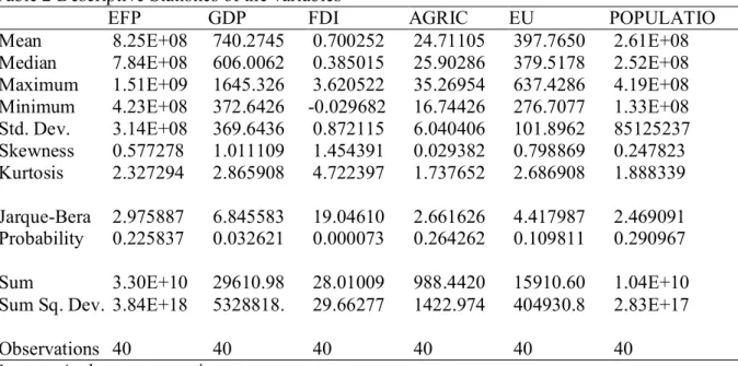
Among the analyses is the descriptive statistics which is presented in Table 2.
Table 2 Descriptive Statistics of the variables
EFP GDP FDI AGRIC EU POPULATIO
Mean 8.25E+08 740.2745 0.700252 24.71105 397.7650 2.61E+08 Median 7.84E+08 606.0062 0.385015 25.90286 379.5178 2.52E+08 Maximum 1.51E+09 1645.326 3.620522 35.26954 637.4286 4.19E+08 Minimum 4.23E+08 372.6426 -0.029682 16.74426 276.7077 1.33E+08 Std. Dev. 3.14E+08 369.6436 0.872115 6.040406 101.8962 85125237 Skewness 0.577278 1.011109 1.454391 0.029382 0.798869 0.247823 Kurtosis 2.327294 2.865908 4.722397 1.737652 2.686908 1.888339
Jarque-Bera 2.975887 6.845583 19.04610 2.661626 4.417987 2.469091 Probability 0.225837 0.032621 0.000073 0.264262 0.109811 0.290967
Sum 3.30E+10 29610.98 28.01009 988.4420 15910.60 1.04E+10
Sum Sq. Dev. 3.84E+18 5328818. 29.66277 1422.974 404930.8 2.83E+17
Observations 40 40 40 40 40 40
Source: Authors computation
From the descriptive analysis it is observed the normality of the analysis by the disposition of the Jarque-Bera and Kutrtosis respectively. Apart from the GDP and FDI with significant outcomes all other variables are not significant for the case of Jarque-Bera showing the normality of the data and test. With the result showing all the variables less than 3 except FDI displays light tail. In addition, the test reports the mean, standard deviation, maximum and minimum with ecological footprint and population showing the highest mean, median and maximum output. FDI displays the minimum output.
14
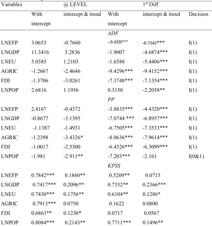
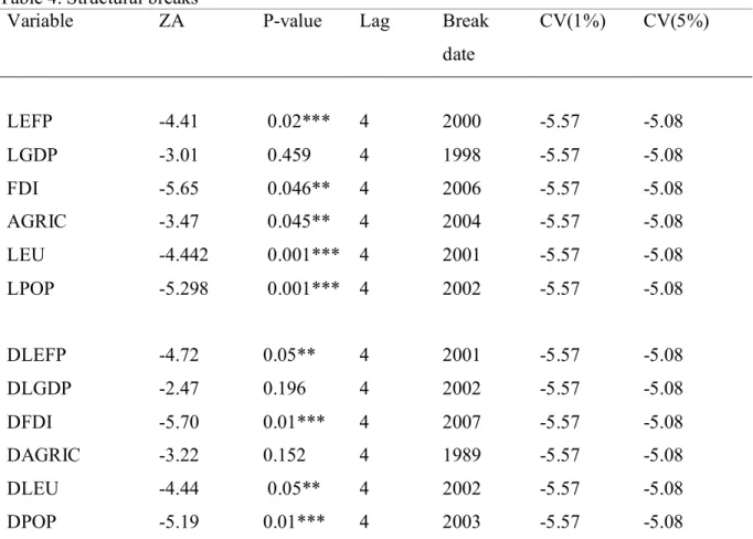
The next test was done to ascertain the stationarity features of the variables and make sure that none of the variables was integrated at order I(2) and the result is displayed in Table 3. This is to be on the same page with the requirement of NARDL that order I(2) is not established among the variables (Shin et al., 2014). The applications utilized in ascertaining the stationarity of this present study are Philip–Perron, (1990), Augmented Dickey-Fuller, (ADF 1981) and Kwiatkwoski Philips-Schmidt-Shin (KPSS 1992). And Zivot and Andrew, 1992 Structural break. The result of the above mentioned tests showed that all the variables are integrated in order I(1) except the agriculture with a mixed order of I(0) and I(1). In other to avoid the problem of biased empirical results capable of emanating from the use of the traditional unit test approaches such as ADF, DF which are weak in the face of structural break, the current study adopts the structural break analysis. This is to accommodate intermediate shocks that has permanent shock on the time series, and if possible get rid of any illogical result from the conventional techniques. Zivot and Andrew (1992) approach which is a modification of Perron P, (1990) approach was utilized and the result is presented in Table 4. With the application of the structural break analysis, it is observed that the variables have unit roots in the existence of the structural changes that took place in 2000, 1998, 20006, 2004, 2001, 2002, 2007, 1989 and 2003. India as a country is known with much structural changes which always leave them with permanent shocks. Over the sample period, the country adopted and implemented several economic and energy policies to improve its economic growth performance. Such policies include the liberalization policies of 1990s and 2000s which was targeted on the trade expansion and investment attraction to the economy for the wellbeing of the country. This really affected the local production and the entire economic performance of the country (India). As for the energy sector, the policies of abolishing the Administrative Price Mechanism (APM) on the 1st of April, 2002 was instrumental for the availability of energy sources such as liquefied petroleum gas (LPG) and other oil for the masses and the manufacturing sectors at the subsidized prices. The 1997/8 global financial meltdown contributed to the Indian structural beak and this date was accounted for in the analysis. The structural changes that took place in the banking sector in 1980 -1990 because of the nationalization of the commercial private banks and the taking over of some distressed private banks by the central bank was part of the policies. Similarly, was the involvement of the International Monetary Fund (IMF) in the local financial activities in India in 1990’s which positively impacted the economic performance of the India’s economy through increased capitalization stability of the financial sector.
15
Table 3. Stationarity Test
Variables @ LEVEL 1st Diff
With intercept
intercept & trend With intercept
intercept & trend Decision
ADF LNEFP 3.0653 -0.7660 --5.4297*** -6.7342*** I(1) LNGDP 11.3416 3.2836 -1.9007 -4.6874*** I(1) LNEU 5.0385 1.2103 -1.6588 -5.4406*** I(1) AGRIC -1.2667 -2.4646 -9.4296*** -9.4152*** I(1) FDI -1.3706 -3.0261 -7.3748*** -7.1354*** I(1) LNPOP 2.6816 1.1936 0.3150 -2.2058** I(1) PP LNEFP 2.4167 -0.4372 -3.8835*** -4.4320*** I(1) LNGDP -0.8677 -3.1395 -7.0744 *** -6.8957*** I(1) LNEU -1.1387 -1.4931 -6.7505*** -7.3533*** I(1) AGRIC -1.2398 -3.4326* -8.0636*** -7.9614*** I(1) FDI -1.0017 -2.5300 -6.4526*** -6.3099*** I(1) LNPOP -1.981 -2.911** -7.203*** -2.161 I(0&1) KPSS LNEFP 0.7842*** 0.1860** 0.5209** 0.0715 LNGDP 0.7417*** 0.2096** 0.7332** 0.2366*** LNEU 0.7430*** 0.1756** 0.6104** 0.1286* AGRIC 0.7913*** 0.0750 0.1622 0.0800 FDI 0.6863** 0.1230* 0.0717 0.0567 LNPOP 0.8084*** 0.2143** 0.7711*** 0.1496**
Notes: a: (*) Significant at the 10%; (**) Significant at the 5%; (***) Significant at the 1%( b):
P-value according to (1) Maclean et al., (1996) one-sided p-P-values (2) Kwiatkowski-Phillips-Schmidt-Shin (1992,)
16
Table 4. Structural breaks
Variable ZA P-value Lag Break
date CV(1%) CV(5%) LEFP -4.41 0.02*** 4 2000 -5.57 -5.08 LGDP -3.01 0.459 4 1998 -5.57 -5.08 FDI -5.65 0.046** 4 2006 -5.57 -5.08 AGRIC -3.47 0.045** 4 2004 -5.57 -5.08 LEU -4.442 0.001*** 4 2001 -5.57 -5.08 LPOP -5.298 0.001*** 4 2002 -5.57 -5.08 DLEFP -4.72 0.05** 4 2001 -5.57 -5.08 DLGDP -2.47 0.196 4 2002 -5.57 -5.08 DFDI -5.70 0.01*** 4 2007 -5.57 -5.08 DAGRIC -3.22 0.152 4 1989 -5.57 -5.08 DLEU -4.44 0.05** 4 2002 -5.57 -5.08 DPOP -5.19 0.01*** 4 2003 -5.57 -5.08
Notes: a: (*) Significant at the 10%; (**) Significant at the 5%; (***) Significant at the 1%( b):
P-value according to (1) Maclean et al., (1996) one-sided p-P-values
Source: Authors computation
4.2 Cointegration and diagnostic results
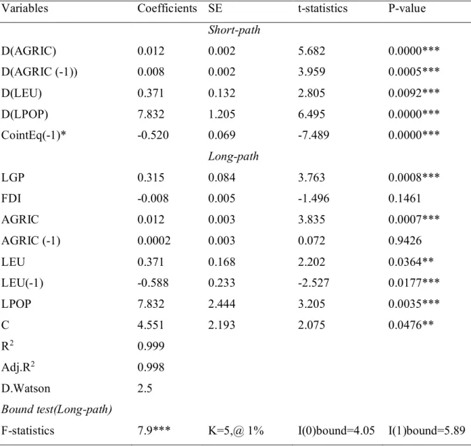
The ARDL results are displayed in Table 6. The goodness of fit of the analysis shows that the selected independent variables (GDP, FDI, AGRICULTURE, ENERGY USE and POPULATION) explain 99.9% (R2 =0.999110) of the ecological footprints while the error term in the model accounts for the rest of the variations in the ecological footprints. The Durbin Watson (DW) test statistics is 2.545 approximately in affirmation of the nonappearance of autocorrelation in the model assessment which indicates that the selected independent variables in the model can describe the deviation in the dependent variable (EFP) in the absence of autocorrelation. The author observed the absence of heteroscedasticity problem from the model. The author equally found the CUSUM and CUSUM of squares well positioned, that is, the blue lines in both figures (1 and 2) well placed inside the two doted red lines. These findings show the reliability, stability and consistency of the empirical outputs. More also, this study found that F-statistics test is greater than the upper critical bound even at 1% level of significance for the case of ARDL. This confirms
17
the existence of cointegration or long run linear relationship among the selected variables for the period of 1975-2016. Even the t-statistics validates the existence of the cointegration among the variables at 1% significant level. These findings from both the F-test and t-test indicate the existence of long-run symmetric relationship in the Indian ecological footprints. The results of both the long run and the short-run are presented in a detailed way below in Table 6. The table contains the result of the above mentioned estimations and diagnostics. The optimal lag length selection was performed with choice of the Akaike Information Criterion (AIC) as a selection criterion for its stronger features above other criteria (Shahbaz &Rahman, 2012). The selected lag was 2 and it is considered good because of the sample size of the study. The result is with the author and will be made available on request. Among the findings of this analysis is the error correction model (ECM) which is highly significant at 1 percent significant level with a negative coefficient of 0.52 (-0.52). This indicates the speed of regulation in reestablishing the disequilibrium in the dynamics model to equilibrium at -0.52%, and the confirmation of the long run relationship that exist among the variables. The effects of the explanatory variables on the LEFP are displayed in the Table 5 and can be interpreted and explained with references as follow: a long run (elasticity) positive and highly significant relationship between the economic growth and ecological footprint. Numerically, a one percent increase in economic growth impacts ecological footprint positively at the rate of 0.32%. This means that economic performance of India is impacting negatively on its environment with the positive association established between EFP and GDP. In other words, as the economic growth is increasing positively, the environmental degradation is increasing. This finding supports the early stage (scale effect stage) of the EKC theory which stated that at this stage the country is encouraging economic growth at the expense of the environment because all attention is towards boosting economic growth which is typical of developing economy like India. In other words, it is a reflection of economic growth and development without attention to the environmental implication of the growth. Some of the developing countries like India most times frame the policies on soft landing of foreign activities into their countries such as foreign investors and trade without same measure on protecting the environment from any unduly activities from the foreigners. The foreign investors will explore all the loopholes to increase their investment and manufacturing activities in the country with less concern on maintaining environment with clean energy. This finding is consonance with the works of Alola, A. A., Yalçiner, K., Alola, U. V., & Saint Akadiri, S. (2019) for large economies of Europe; Emir and Bekun, (2018) for Romanian, and Udemba EN (2019) for China. A long run (elasticity) negative but not significant is observed between ecological footprint and foreign direct investment. This is a good trend for both the economic and the environmental performance of the country even though the negative relationship that exist between the ecological footprint and FDI is not yet significant so far there is a long run relationship between the two indicators. This is a typical example of transition economy where there is awakening consciousness of the masses on the need for a cleaner energy for a better environment. This can be seen from the second (structural or composition effect stage) stage of the growth and development as derived from the EKC theory. At this stage there is a shift from crude means of handling some sectors of the economy such as agriculture to a more industrialized means with manufacturing sectors and investments (domestic and foreign) rising more than other sectors. This output is in affirmation with the exposes of Zhang, W.B., 2018; Danish et al. 2018; Sarkodie and Strezov, 2019; Udemba E.N, 2019; Shahbaz and
18
Balsalobre, (2019) for MENA; Paramati, S. R., Apergis, N., & Ummalla, M. (2017) for EU, G20 and OECD; Pazienza, (2015) for OECD and Udemba et al., (2019) for Indonesia. Also, agricultural sector is found impacting negatively on the environmental performance of India with a positively significant relationship (both in the short and long run) that exist between agricultural sector and ecological footprint. Numerically, a one percent increase in agricultural activities (as it relates to
both fishing and forest activities) increases ecological footprint by 0.12%. This amounts to increase
in environmental dilapidations in India. The finding supports the findings of Dogan, (2016) for Turkish; Liu et al., (2017b) for ASEAN and Ullah et al., (2018) for the Pakistan. This is very much understood in the case of the highly populated country like India whose majority of its masses are into agricultural activities such as farming, fishing and cattle rearing. Most of these activities such as rice farming which involves the usage of fertilizers and other chemical substances for the quick and large production contaminate the environment. The fishing and cattle rearing contaminate the water bodies and impact negatively on the grazing lands and all these are part of ecological footprint. The author also found a positive and highly significant relationship (short run and long run) among energy use, population and ecological footprint. Both variables (energy use and population) are observed impacting negatively on the environmental performance of India with a positive relationship that is already established between the variables and the ecological footprint. This is not far-fetched from the definition of the ecological footprint by the Global Footprint Network (2018) as it relates to population. Ecological footprint is described as extent of a geographical area of organically useful earth and water a group of people (population), or action needed to yield all the resources it consumes. Among the pronounced features of India is its population which is among the determinant of the environmental performance through the activities of the populace in other sectors (e.g. agricultural sector) and the energy utilization of the population. According to statistics from Carbon Brief Profile (2019), India is a home to 18 percent of the world’s population, but has only 2.4 percent of the land area with a great amount of pressure being placed on all the country’s resources. This is part of definition of ecological footprint. Numerically put, a one percent increase in population increases the ecological footprint by 7.8%. India as a country on the speed lane of economic growth increased its energy consumption from different sources mainly nonrenewable energies such as coal, crude oil and others. These non-renewable energies emit higher percentage of pollutant emissions into the environment via air which hamper the positive performance of the environment. This can be seen from among the policies of Indian government in the energy sector. This comes with abolishing of the Administrative Price Mechanism (APM) on the 1st of April, 2002 which was instrumental for the availability of energy sources such as liquefied petroleum gas (LPG) and other oil for the masses and the manufacturing sectors at the subsidized prices. Such policies trigger the energy consumption which when it is not moderated affect the environmental performance negatively and this is the picture of the finding of this study with positive relationship that exist between the energy use and ecological footprint. Numerically, a one percent of increase in energy use increases the ecological footprint by 0.3%. This finding supports the findings of Al-mulali and Ozturk, (2015) for the 14 MENA; Ozturk, et al., (2016) for the case of 144 countries; Bekun, F. V., Alola, A. A., & Sarkodie, S. A. (2019) for 16 EU countries; Akadiri, A. C., Saint Akadiri, S., & Gungor, H. (2019a) for Saudi Arabia; Sarkodie, S. A., & Strezov, V. (2019) for developing countries.
19
However, the findings of this study cut across different sectors ranging from agricultural sector to energy sector with interesting relationships which exposes the hiding nature of environmental performance, and call for a good policy frame work targeting the reduction of ecological footprint.
Table 5. Bound with F-test linear and nonlinear cointegration
Panel A. F-test output for the ARDL models Panel A. F-test output for the NARDL models Cointegration hypothesis F-stat. Upper. Bound Cointegration hypothesis F-stat. Upper. Bound F(LEFPt/ LGDPt,
FDIt,AGRICt,LEUt, LPOPt)
7.9*** 5.2 F(LEFPt/ LGDPt +, LGDPt - , FDIt+, FDIt-AGRICt +, AGRICt -,LEUt +, LEUt - ,LPOPt + , LPOPt -)
5.7 7.2
Table 6. ARDL assessments of EFP equation
Variables Coefficients SE t-statistics P-value
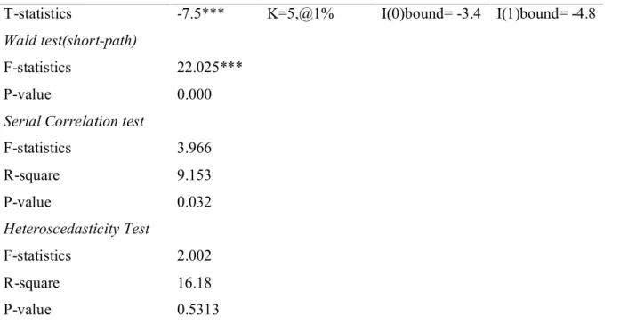
Short-path D(AGRIC) 0.012 0.002 5.682 0.0000*** D(AGRIC (-1)) 0.008 0.002 3.959 0.0005*** D(LEU) 0.371 0.132 2.805 0.0092*** D(LPOP) 7.832 1.205 6.495 0.0000*** CointEq(-1)* -0.520 0.069 -7.489 0.0000*** Long-path LGP 0.315 0.084 3.763 0.0008*** FDI -0.008 0.005 -1.496 0.1461 AGRIC 0.012 0.003 3.835 0.0007*** AGRIC (-1) 0.0002 0.003 0.072 0.9426 LEU 0.371 0.168 2.202 0.0364** LEU(-1) -0.588 0.233 -2.527 0.0177*** LPOP 7.832 2.444 3.205 0.0035*** C 4.551 2.193 2.075 0.0476** R2 0.999 Adj.R2 0.998 D.Watson 2.5 Bound test(Long-path)
20
T-statistics -7.5*** K=5,@1% I(0)bound= -3.4 I(1)bound= -4.8
Wald test(short-path)
F-statistics 22.025***
P-value 0.000
Serial Correlation test
F-statistics 3.966 R-square 9.153 P-value 0.032 Heteroscedasticity Test F-statistics 2.002 R-square 16.18 P-value 0.5313
Note: *, **, *** Denotes rejection of the null hypothesis at the 1%, 5% and 10% Sources: Authors computation
4.3. Diagnostic tests (CUSUM and CUSUM of squares)
-16 -12 -8 -4 0 4 8 12 16 88 90 92 94 96 98 00 02 04 06 08 10 12 14 16 CUSUM 5% Significance -0.4 -0.2 0.0 0.2 0.4 0.6 0.8 1.0 1.2 1.4 88 90 92 94 96 98 00 02 04 06 08 10 12 14 16
CUSUM of Squares 5% Significance
Figure 1: CUSUM residual graphical plot Figure 2: CUSUM square residual graphical plot 4.4. Granger Causality
The linear ARDL estimation and analysis can only indicate the relationship impact among the selected variables but lack the power to exhibit the direct transmission or feedback that exist among the variables. Even though, ECM is considered a test of short path causality among the variables it is not sufficient to determine the direct transmission between the variables. This led to the adaptation of Granger causality to explicitly show the direct transmission among the variables. However, this present study does not entirely depend on granger causality. Author applied many methods (of which granger causality is among them) in trying to arrive at efficient results and
21
validation of the findings. The author applied granger causality for a clear identification of the direction in the relationship that exist between the dependent and independent variables and to determine the variable that causes the other.
The author applied VAR approach to estimate the Granger causality. The current paper adopts the Block exogenuity Wald test (long path causality) for the granger causality test and the output is seen from the Table 7 below.
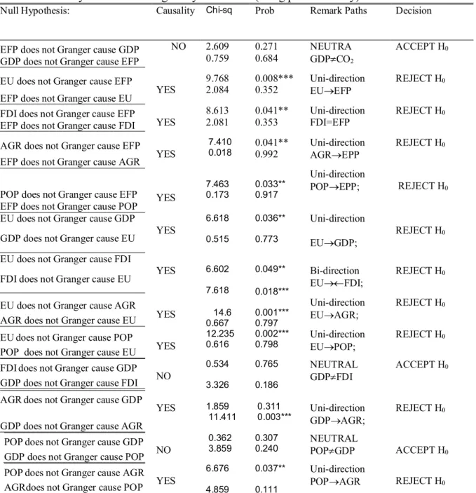
Table 7. Causality test/ Block exogenuity Wald Test (Long path causality)
Null Hypothesis: Causality Chi-sq Prob Remark Paths Decision
EFP does not Granger cause GDP GDP does not Granger cause EFP
NO 2.609 0.759 0.271 0.684 NEUTRA GDPCO2 ACCEPT H0
EU does not Granger cause EFP
EFP does not Granger cause EU YES
9.768 2.084 0.008*** 0.352 Uni-direction EUEFP REJECT H0
FDI does not Granger cause EFP
EFP does not Granger cause FDI YES
8.613 2.081 0.041** 0.353 Uni-direction FDI=EFP REJECT H0
AGR does not Granger cause EFP
EFP does not Granger cause AGR YES
7.410 0.018 0.041** 0.992 Uni-direction AGREPP REJECT H0
POP does not Granger cause EFP
EFP does not Granger cause POP YES
7.463 0.173 0.033** 0.917 Uni-direction POPEPP; REJECT H0
EU does not Granger cause GDP
GDP does not Granger cause EU YES
6.618 0.515 0.036** 0.773 Uni-direction EUGDP; REJECT H0 EU does not Granger cause FDI
FDI does not Granger cause EU YES
6.602 7.618 0.049** 0.018*** Bi-direction EUFDI; REJECT H0
EU does not Granger cause AGR
AGR does not Granger cause EU YES 14.60.667 0.001***0.797
Uni-direction EUAGR;
REJECT H0
EUdoes not Granger cause POP
POP does not Granger cause EU YES
12.235 0.616 0.002*** 0.798 Uni-direction EUPOP; REJECT H0
FDIdoes not Granger cause GDP GDP does not Granger cause FDI NO
0.534 3.326 0.765 0.186 NEUTRAL GDPFDI ACCEPT H0
AGRdoes not Granger cause GDP GDP does not Granger cause AGR
YES 1.859 11.411
0.311
0.003*** Uni-direction GDPAGR; REJECT H0
POPdoes not Granger cause GDP GDP does not Granger cause POP NO
0.362 3.859 0.307 0.240 NEUTRAL POPGDP ACCEPT H0 POPdoes not Granger cause AGR
AGRdoes not Granger cause POP YES
6.676 4.859 0.037** 0.111 Uni-direction POPAGR REJECT H0
Notes: the statement under Null Hypothesis are all definition of hypothesis which will be valid or not based on the outcome of P-value and expressed in the decision. The decision is made at 5%.
22
The Remark paths clearly show the direction of the causal effects (bi-directional or unidirectional). ***p<0.01, **p<0.05, *p<0.10.
The output of the causality estimation is presented in Table 7 above. The output gives credence to the findings of the EFP model of equation (1) which is displayed in the linear ARDL table. The result shows a one-way transmission passing to EFP from EU, FDI, AGRIC AND POPULATION. Also, a one-way causality is seen passing to GDP, AGRIC, POPULATION from energy use, and from population to agriculture. More interesting result is the two-way transmission passing between energy use and foreign direct investment. This shows that both variables are impacting each other directly and to the good of both economic performance and environmental performance, hence energy use is transmitting to GDP, and FDI has negative relationship with ecological footprint depicting reducing of environmental damage as FDI upsurge. These outcomes indicate that ecological footprint of India is determined by the selected variable (energy use, foreign direct
investment, agriculture sector and population). The finding really exposes the direction of the
relationship that existed among the variables. This finding also exposes the impact of energy utilization in India, and this supports the cited structural break impact of energy reform policy of 2000’s which sees to the leveraging of the price of the energy sources and making it accessible by both individuals and industries. Hence, energy use is transmitting to GDP, AGRIC and POPULATION. The typical example of the ecological footprint is the impact of the population on the land and water and to the resources as put by Global Footprint Network (2018). This is not far-fetched from the definition of the ecological footprint by the Global Footprint Network (2018) as it relates to population These findings support findings of Al-mulali and Ozturk, (2015) for the 14 MENA; Ozturk, et al., (2016) for the case of 144 countries; Bekun et al., (2019) for 16 EU countries; Sarkodie & Strezov (2019); Udemba EN (2019) for China.
5. Conclusion
According to Carbon Brief Profile report (2019), India has been identified as the world 3rd largest emitter of greenhouse gases (GHG’s) after China and the US. Its emissions are derived from energy sources such as coal power plant, rice factories and cattle farming and all these sources are classified under index as ecological footprint. Following the Paris agreement and India pledge as among the stakeholders at the global climate talks, and how speed the India ratified the Paris Agreement within a year on the 2nd of October, 2016, it is essential to investigate the country’s (India) commitment in reducing its emission towards enhancing a positive environmental performance. Recently, there is increased awareness in renewable or clean energy investments because of the environmental concerns. Previous researches on the performance of environment have been focused on the utilization of single indicator such as pollutant emission, carbon emissions, fossil fuel and others to proxy and measure the environmental impact which is weak in giving a clear and total submission of the dilapidations in the environment. Following this pitfall on the side of measuring the environmental effect, this present paper has considered ecological footprint a more reliable indicator for accounting for the environmental quality because of its accommodation of many emissions sources as one indicator. The current paper utilizes different approaches to see to the richness of the study. Both linear ARDL (Symmetric) and nonlinear ARDL (Asymmetric) were selected simultaneously for this study but at a later stage after bound
23
cointegration estimation, the NARDL was dropped because of its inability to sustain the claim of cointegration from the model of our interest (EFP model) in the analysis. The rest of the analyses were based on liner ARDL model (short-run and long-run) with diagnostic tests, Granger causality estimation. The study and the results derived are consistent with the hypothesis of this work which is in line with the expectations of the author except for the case of foreign direct investment which is impacting favorably on the environmental performance with the establishment of negative relationship with the ecological footprint. This is a good story for the Indian authority, it shows the consciousness of the policy makers in framing an environment friendly policies in line with foreign investors’ engagements in the country. The output from both ARDL and the granger causality points out that India is still in between the scale effect stage and the transitional stage of development with much interest in economic growth and development but little or no interest in the environmental performance, hence the economic growth (GDP) is increasing (positive) and the ecological footprint is increasing (positive). The findings of this study portray the sensitivity of energy use in India’s economic and environmental performance, hence energy is transmitting directly to all the variables (AGRIC, ENERGY USE, and POPULATION) with a feedback transmission existing between energy use and foreign investment (FDI), and also, a positive link is established between energy use and the ecological footprint. The agriculture and population which are considered main ingredients in the formation of ecological footprint are consistent with the authors hypothesis, hence the output in both ARDL (positive link to EFP) and granger causality (one-way causality from AGRIC and POPULATION to ECOLOGICAL FOOTPRINT) depicts the authors claim and hypothesis.
At this point, the policy development and implementation of India should focus on attracting and regulating FDI with a good environmental condition. The policy will look towards sustaining both economic performance and good environmental performance. Increase taxation on the energy sources that emit high pollution while reduce tax on the low carbon energy sources. The Indian authority should look into the agriculture sector and the population and frame a policy that will encourage the boosting of the agricultural performance with less harm to the environment as this sector is seen a very vital sector in India. A campaign to discourage population growth such as child birth control is needed in a country like India. Again, there is a need for a revisit to energy policy in India as energy use is seen dominating all the sectors in India. Policies that will see to the shifting of energy use to a cleaner energy sources such as wind and solar energy sources are to be framed and implemented.
Conclusively, as India is working towards achieving its economic target, the country should also up its game in bettering its environmental performance.
24 Appendix
Definition of terms
Terms Full meaning
ARDL Autoregressive Distributed Lag
NARDL Nonlinear Autoregressive Distributed Lag
FDI Foreign Direct Investment.
GC Granger Causality
GDP Gross Domestic Product (rep. as GDP per
capita)
EFP=ecological footprint Ecological Footprint (The Global Footprint
Network (2018) describes the ecological footprint as “a measure of how much area of biologically productive land and water an individual, population, or activity requires to produce all the resources it consumes and to absorb the waste it generates, using
prevailing technology and resource management practices).
C02 = carbon emission Carbon emission (According to World Bank,
2018, Carbon dioxide emissions are those
stemming from the burning of fossil fuels and the manufacture of cement. They include carbon dioxide produced during consumption ofsolid, liquid, and gas fuels and gas flaring.)
Pollution = environmental degradation According to Environmental Management, 2017 “Environmental pollution is defined as "the contamination of the physical and biological components of the
earth/atmosphere system to such an extent that normal environmental processes are adversely affected.".
AIC Akaike Information Criterion
ADF Augmented Dickey-Fuller test
PP Philip-perron,
KPSS Kwiatkwoski Philip-Schmidt-Shin
EU Energy use
DW Durbin Watson
POP Population
25 References
Ali, S., Yusop, Z., Kaliappan, S. R., & Chin, L. (2020). Dynamic common correlated effects of trade openness, FDI, and institutional performance on environmental quality: evidence from OIC countries. Environmental Science and Pollution Research, 1-12.)
Al-Mulali, U., Saboori, B., & Ozturk, I. (2015). Investigating the environmental Kuznets curve hypothesis in Vietnam. Energy Policy, 76, 123-131.
Alola, A. A., Yalçiner, K., Alola, U. V., & Saint Akadiri, S. (2019). The role of renewable energy, immigration and real income in environmental sustainability target. Evidence from Europe largest states. Science of The Total Environment, 674, 307-315.
Álvarez-Herránz, A., Balsalobre, D., Cantos, J. M., & Shahbaz, M. (2017). Energy innovations-GHG emissions nexus: fresh empirical evidence from OECD countries. Energy Policy, 101, 90-100.
Bagliani, M., Bravo, G., & Dalmazzone, S. (2008). A consumption-based approach to environmental Kuznets curves using the ecological footprint indicator. Ecological
Economics, 65(3), 650-661.
Baloch, M. A., Zhang, J., Iqbal, K., & Iqbal, Z. (2019). The effect of financial development on ecological footprint in BRI countries: evidence from panel data estimation. Environmental Science
and Pollution Research, 26(6), 6199-6208
Banerjee, A., Dolado, J., & Mestre, R. (1998). Error‐correction mechanism tests for cointegration in a single‐equation framework. Journal of time series analysis, 19(3), 267-283.
Banerjee, A., Dolado, J., & Mestre, R. (1998). Error‐correction mechanism tests for cointegration in a single‐equation framework. Journal of time series analysis, 19(3), 267-283.
Bekun, F. V., Alola, A. A., & Sarkodie, S. A. (2019). Toward a sustainable environment: Nexus between CO2 emissions, resource rent, renewable and nonrenewable energy in 16-EU countries. Science of the Total Environment, 657, 1023-1029.
Bello, M. O., Solarin, S. A., & Yen, Y. Y. (2018). The impact of electricity consumption on CO2 emission, carbon footprint, water footprint and ecological footprint: the role of hydropower in an emerging economy. Journal of environmental management, 219, 218-230.
Danish, Wang, Z., (2018). Dynamic relationship between tourism, economic growth, and environmental quality, Journal of Sustainable Tourism, 26, 11, 1928-1943.
Destek, M. A., & Okumus, I. (2019). Does pollution haven hypothesis hold in newly industrialized countries? Evidence from ecological footprint. Environmental Science and Pollution
Research, 26(23), 23689-23695
Dickey, D. A., & Fuller, W. A. (1979). Distribution of the estimators for autoregressive time series with a unit root. Journal of the American statistical association, 74(366a), 427-431.