Cooling and heating degree days in the US: The role of
macroeconomic variables and its impact on environmental
sustainability.
Andrew Adewale Alola
Faculty of Economics, and Administrative and Social Sciences, Istanbul Gelisim University, Istanbul, Turkey.
Email: [email protected]
Seyi Saint Akadiri
1College of Business, Westcliff University, Irvine, California, United States.
Email: [email protected]
Ada Chigozie Akadiri
Faculty of Business and Economics, Department of Economics, Famagusta, Eastern Mediterranean University, North Cyprus, via Mersin 10, Turkey.
Email: [email protected]
Uju Violet Alola
Faculty of Economics, Administrative and Administrative and Social Sciences, Istanbul Gelisim University, Istanbul, Turkey.
Email: [email protected]
Ayodeji Samson Fatigun
College of Business, Westcliff University, Irvine, California, United States.
Email: [email protected]
Abstract:
1
Corresponding author: Seyi Saint Akadiri.
Beyond employing the degree days for assessing climatic situations and the expected energy needs, a subtle concern is the underpinning of the role of the environmental sustainability amidst socio-economic activities on the degree days. As such, the current study is design to examine the role of fossil fuel energy consumption, ecological footprint, and urban population on the degree days viz-a-vis the cooling and heating days in the United States over the period 1960-2015. The Autoregressive Distributed Lag bound testing model employed reveals the importance of the ecological footprint, fossil fuel energy consumption, and urban population on the cooling and heating degree days of the United States. Result posits that each of fossil fuel and the urban population plays a positive and negative role as regard the cooling degree days and the heating degree days respectively, especially in the long run. Importantly, the empirical results support the argument that the increase in the consumption of the fossil fuel sources of energies are responsible to cause more cooling degree days, thus resulting to longer and hotter periods in the United States but vice versa for the heating degree days. Similarly, the investigation outcome drams from the argument that the increase in the urban population is a potential cause of high environmental temperature, thus responsible for lengthy heat periods (cooling degree days) and resulting in more energy needs and technologies for cooling. Expectedly, the reverse is the case for the heating degree days, especially in the long-run. As a policy standpoint, policymakers are to further adopt improved and effective guideline for housing and building constructions that are weather specifics. In formulating policy vehicle for each of the seasonal dynamics, the economic benefits of each of the climatic measurements should be considered especially for both the short- and long-run environmental sustainability.
Keywords: Sustainable energy; ecological footprint; urban population; heat energy; time series.
1. Introduction
The twin problems of global warming and climate change have been a subject of discussion, deliberation and of concern among individuals, academic scholars, researchers, governments, private institutions and policymakers in recent time. The reason for this deliberation is not farfetched and can be traced to the potential threat global warming and climate change possess for the environment and ecosystem at large (Wang and Chen, 2014). According to the Intergovernmental Panel on Climate Change (IPCC) the rise in annual temperature between the periods 1960s-2100s has been projected to be within the interval of 1 - 7 K within several carbon dioxide emissions synopsis (Solomon et al., 2007). It was further argued that, solar radiation, wind and humidity would possibly change overtime, in addition to variations in temperature, which is as a result of an increase in metric ton per capita of CO2 emissions generated (Karl,
Melillo and Peterson, 2009).
Energy consumption would exercise large effect on residential energy demand for cooling and heating due to variation in outdoor conditions (Christenson, Manz & Gyalistras, 2006). Le Compte and Warren (1981), Quayle and Diaz (1980) and Sailor and Munoz (1997) in their various empirical analysis have reported that energy consumption is highly associated with degree days for both cooling and heating. For an average outdoor temperature lower than 18◦C, most buildings require heating to maintain a 21◦C indoor temperature, and vice versa. The selection of 18◦C as the base outdoor temperature is as a result of the additional heat generated by occupants and their activities, leading to an average indoor temperature of 21◦C at 18◦C outdoors. On the other hand, the level of energy demand/consumed for heating and cooling is anticipated to decrease and/or increase, due to decrease and/or increase in global warming (Wilbanks, 2009). Although, the effect of climate change on cooling and heating energy demand of different states and/or locations are anticipated to differ because of their contrasting climate.
Thus, a detailed empirical analysis is required to understand factors that determine the cooling and heating energy demand and the impact of climate change on the residential energy usage. This study seeks to fill this gap in energy literature.
Going by the latest reports from the Residential Energy Consumption Survey (RECS) in 2015 air conditioning and space heating on average, accounted for about 54 percent of the United States residential end-use energy consumption and expenditures (Energy International Agency (EIA), 2018). It is no news that variation in outdoor air-temperature is associated and are known to exercise significant effect on climate-related building energy consumption (see Fung, Lam, Hung et al 2006; Valor, Meneu and Caselles 2001) and thus have a significant impact on the population, the level of non-renewable and renewable energy demanded/consumed and on the metric ton per capita of carbon emissions generated. Thus, it is of interest to examine the role these macroeconomic variables play as a determinant, spatial patterns and the magnitude of cooling and heating demand, on environmental degradation most especially in the case of United States.
This is due to the fact that, recently, the United States Climate Change Science Program investigated about 20 United States building energy sector responsiveness to global warming and concluded that, the aggregate forecasted average over the surveyed public studies is roughly 5 to 20 percent energy increase for cooling per 1 C of air-temperature increase and about 9 percent energy decrease for heating of air-temperature decrease. After all, the world average surface temperature in the year 2100 is anticipated to increase by 2.6 to 48 C as argued by Collins et al (2013) under the Representative Concentration Pathways (RCP) 8.5 unabated high emissions framework, climate change is forecasted to change the existing balance among household cooling and heating needs all over the United States, likely triggering states with lower weathers
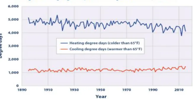
to cosy and change some states from predominantly heating to predominantly cooling demand (see Auffhammer & Mansur 2014; Wang & Chen 2014; Collins et al 2013; Wilbanks et al 2008). Heating degree days have declined in the contiguous United States, particularly in recent years, as the climate has warmed. This change suggests that heating needs have decreased overall. While in general, the cooling degree days have increased over the past 100 years. The increase is most noticeable over the past few decades, suggesting that air conditioning energy demand has also been increasing recently. Heating degree days have generally decreased and cooling degree days have generally increased throughout the North and West. The Southeast, with the exception of the state of Florida, which have seen the opposite: more heating degree days and fewer cooling degree days. Figure 1 show the cooling and heating degree days between the periods 1895-2015.
<Insert Figure 1>
Figure 1: Cooling and heating degree days in the contiguous 48 States between 1895 -2015.
Although, the cooling and heating degree days approach has been argued to be related with specific shortcomings (see Day 2016; Day & Karayiannis 1998). These variables precisely take into consideration the severity and duration of weather conditions (Day, 2006; Mourshed, 2014), therefore, the variables are becoming a functional tool for appraising and assessing residential cooling and heating demand in addition to outdoor thermal consolation. In this study, we mainly focus and investigate factors (macroeconomic variables) that determine and/or contribute to the heating and cooling demand in the case of the United States, and not interested in evaluating the related energy costs and requirements unlike in previous studies (see Day 2016; Mourshed, 2014; Day & Karayiannis 1998).
This study contributes empirically and methodologically to the existing literature on cooling and heating degree days in twofold; First, this study is first or among the few studies that evaluate the macroeconomic factors that determine and contribute to the cooling and heating degree days in the case of the United States. Second, in order to carry out comprehensive impacts of the explanatory variables on the dependent variables, this study employs Autoregressive Distributed Lag (ARDL) model that produces short-run and long-run dynamic and robust coefficients with the speed of adjustment over the time horizon. ARDL is employed to confirm whether the explanatory variables exhibit short-run or long-run impact on the dependent variables (cooling and heating demand). Since, the knowledge of the specific periods at which these explanatory variables contribute (if statistically significant) will assist the policymakers to make valuable residential cooling/heating demand forecast along with sound environmental policies that would help to mitigate climate change impacts for the immediate and future generation.
The remaining part of this study is schedule as follow: Part 2 discuss the United States and its weather forecast. Part 3 entails data, data source and empirical approaches utilized, while part 4 report the results and discuss empirical findings. Part 5 concludes the study with policy recommendations.
2. United States and its Future Weather Conditions in brief
According to Rasmussen, Meinshausen and Kopp (2016) future climate change forecast, the United States has been forecasted to expose to rising warmer summers for the next 100 years. In between the year 1981-2010, most especially between the months June to August, the United States average summer temperature rose to about 75°F. If this situation persists, the climate change for the years 2030 to 2049, the country summer average temperatures may probably
increase by an additional 2 to 5°F under RCP 8.5 which translate to an average of 77 to 80°F respectively.
With a progressive world greenhouse gas emissions reduction trajectory (RCP 2.6), the increase would probably be restricted between 2 to 3°F, with a country summer average of 77 to 78°F. The nation averages, although, reveal much more radical regional and local variations in weather condition. The South, clarified as the West South Central, East South Central, and Southern Atlantic Census regions, for an instance, may probably experience a swing from its notable mean summer weather condition of 75 to 85°F to a mean in the 80 to 90°F range under the RCP 8.5. On the other hand, according to Rasmussen et al (2016) the West South-Central region such as Louisiana, Texas, Oklahoma and Arkansas are forecasted to experience substantial warming, with probably summer weather conditions increasing from a notable mean of 82°F to 85-87°F by the year 2040 under RCP 8.5.
Furthermore, the US is predicted to also experience an increase in the amount of extreme heat days those with maximum temperatures over 95°F. In decades ago, the average American citizen and/or population has been exposed to about 15 days (two weeks) every year of hotter or 95°F (Rasmussen et al 2016). The average America population by the year 2040, has been argued to experience 25 to 40 days annually under RCP 8.5 program. While West South-Central region and Texas should be ready to face 2 to 3 months of days topping 95°F, which is historic in nature for those regions. In addition, an increasing number of counties in the Arizona, southern Texas and California should be ready to face about 4 months or more of hotter days reaching 95°F on average every year.
In addition, there are common high predicted variations in average winter weather conditions and the decrease in the number of exceptionally cooling degree days across all over the United States. Similarly, the Northern States have experienced greatest swing, with average winter weather condition probably increasing from and between 2.9 to 6.5°F in the Northeast by mid-century under RCP 8.5 program. It is paramount to state here that, out of the 25 States that are presently experiencing sub-freezing average winter weather conditions, only six states such as Alaska, North Dakota, Vermont, Minnesota, Wisconsin and Maine by the end of the century are still possibly to do so under RCP 8.5.
3. Materials and Methods
3.1 Materials
The cooling and heating degree days (the CDD and HDD respectively) are not new climate rhetoric, rather the reported significant dynamics in the measurements across the globe has remained the 21st century challenge of the climatologist, environmentalist, and other stakeholders. The United States (38 00 N, 97 00 W with a mostly temperate climate and total area of 9, 833, 517 square kilometers) (Central Intelligence Agency, CIA, 2019) is commonly a 18oC heating degree-days but the average value of the temperature varies by geographical location across the States. In a normal situation, the outdoor temperatures are expectedly different from the indoors, thus affecting daily lives in dynamic ways. These effects are largely responsible for the human demand for heating and air conditioning because of the dynamic nature of the human comfort levels. For instance, the Energy Information Administration (EIA, 2015) implied that about 48% of the total energy consumed are expanded on heating and cooling the household spaces of the American consumers. However, a baseline temperature for indoor comfort of 65oF (18.33oC) is employed for the comparative measurement of daily average
outdoor temperature known as the ‘degree day’. For instance, if different days’ temperature is measured as 85oF (29.44oC) and 30oF(-1.111oC), then the ‘degree days’ are respectively 20oF (-6.667oC) higher (85oF-65oF = 20oF) and 35oF (1.667oC) lower (30oF-65oF = -35oF). The implication is that the first day requires energy source (cooling device) to attain a 20oF (-6.667oC) cooling degree days while the other day requires energy source (heating device) to attain 35oF (-1.111oC) heating degree days.
3.1.1 Data Description
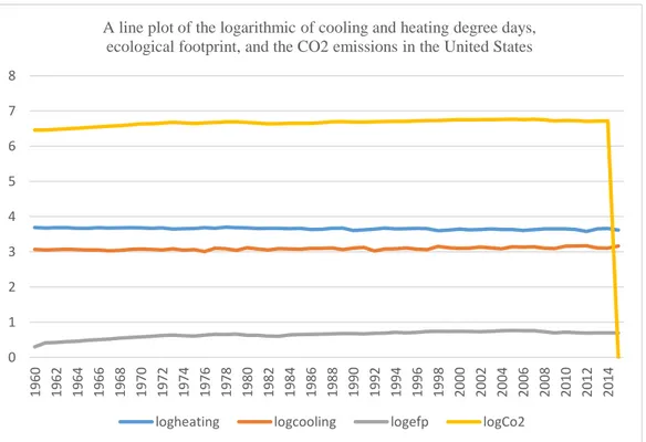
In respect to the measurement of the heating and cooling degree days, studies have noted the significant effect of the climate change due to fossil energy consumption, and other human activities on the ecosystem on the global cooling and heating days, thus posing concerns on the global environmental sustainability. In underpinning this environmental sustainability challenge, the current study employs the cooling and heating degree days for the United States (from the aggregate of 48 States, available in https://www.epa.gov/climate-indicators/climate-change-indicators-heating-and-cooling-degree-days) as separate dependent variable. The independent variables utilized in the study include the ecological footprint, the fossil fuel energy consumption, and the urban population. These series which were retrieved from different sources is span over the period of 1960 to 2015. In Table 1, the variables employed, the unit of measurement and sources are further presented in details. The common statistics and the line plot of the series are respectively presented as Table 2 and Figure 2.
<Insert Table 1> <Insert Table 2>
3.2 Method
3.2.1 Model Specifications
Given that environmental conditions (which include environmental quality/degradation) are being widely investigated in the literature, empirical studies have continued to show that climate change has continued to be expressed as function of income growth, fossil fuel energy consumption, renewable energy consumption, and even population among others (Alola, 2019a; Alola, 2019b; Alola, Bekun & Sarkodie, 2019; Alola, et al, 2019; Bekun, Alola, & Sarkodie, Emir & Bekun, 2019; 2019; Saint Akadiri, Alola & Akadiri, 2019; Saint Akadiri, et al., 2019).
In advancing the study of environmental sustainability, the measurement of the CDD and the HDD are being considered in recent studies. For instance, Mastrucci et al., (2019) opined that the energy demand for space cooling is potentially captured by the technological intensity driver, the structural intensity driver and the activity driver. According to Mastrucci et al., (2019), the above categorized drivers are potentially disaggregated into population, building features to measure the energy intensity. Subsequent studies such as Otsuka and Goto (2018) and Spinoni et al (2018) reserved that population plays a significant role in determining the degree days and that such impact is mostly dependent on the region under consideration. Also, in addition to the importance of socio-economic factors as identified by Labriet et al (2015), the study identified considered that fossil fuel energy consumption is primarily the source of the CO2 emissions.
Hence, considering that De Rosa et al (2015) employed a time series modeling of the degree days as the function of trend and seasonality, the current study considers that the CDD and HDD are both expressed below as a function of ecological footprint, fossil fuel energy consumption, and the urban population of the United States. Thus,
, , ,, UPOP, i t i t i t i t CDD f fossil efp (1) and
, , ,, UPOP, i t i t i t i t HDD f fossil efp (2)where the FOSSIL, EFP, UPOP are the fossil fuel energy consumption, ecological footprint, and urban population respectively for the United States (i) over the period t i.e t = 1960, 1961,…, 2015. However, the models (1) and (2) are both transformed to natural logarithmic such that the effect of potential heteroscedasticity is eliminated in the estimations.
3.2.2 The ARDL-Bound Test
Prior to adapting the ARDL bound approach for the estimation of the models (1) and (2) above, the stationarity test is employed as the preliminary test. In this case, the augmented Dickey & Fuller (1979)-the ADF and Kwiatkowski, Phillips, Schmidt & Shin (1992)-the KPSS were both employed to investigate the stationarity of the series. The result of the estimation is presented in Table 1. The results present the order of integration of the variables (mixed order of integration), thus alluring to the suitability of the ARDL bound test approach. The ARDL test approach is also suitable because it presents the dynamic relationship as well as the long-run and short-run relationship. This is because a dynamic unrestricted error correction model from the ARDL bounds testing technique is obtained from a simple linear transformation without losing the information of the long-run dynamics.
Therefore, the empirical representation of the ARDL bound test approach to cointegration after transforming the above models (1) and (2) to the natural logarithmic forms are presented as equation (3) and (4) below, i.e
1 1 1 1 1
ln
CDD
t
CDDCDD
t
fossillnfossil
t
efplnefp
t
UPOPupop
t1 0 0
lnfossil lnefp lnupop
p q r i t i j t j k t k t i j k
(3) and 1 1 1 1 1lnH
DD
t
CDDHDD
t
fossillnfossil
t
efplnefp
t
UPOPupop
t
1 0 0
lnfossil lnefp lnupop
p q r i t i j t j k t k t i j k
(4) where ln represents the natural logarithmic transformation of the respective variables,
t is the stochastic terms. Accordingly, Pesaran, Shin & Smith (2001) states that ARDL bound test cointegration estimate presents the F-statistics which is essentially compared with the estimated lower and upper critical bounds values. As such, the null hypothesis is specified as an assumption of no cointegration among the series against its alternative (i.e the presence of cointegration relationship among the series). Hence, the hypotheses are presented in Eq. (5) as follows:0
1
0 0
CDD fossil efp UPOP CDD fossil efp UPOP
H H (5)
If the estimated F-statistics is greater than the upper critical bounds value, then, cointegration relationship is present among the series and vice versa. Thus, there is statistical evidence of cointegration if the estimated F-statistics is greater than the upper critical bounds value, and vice versa.
Furthermore, we employ the suitability of the vector error correction model (VECM) for Granger causality testing approach especially since the variables are integrated at first order and there is statistical evidence of long-run cointegration relationship among the series. Hence, the employed VECM Granger causality method is specified as follows in Equation (6):
1 1 11 12 13 14 1 2 21 22 23 24 1 31 32 33 34 3 1 41 42 43 44 4 1 ln ln lnfossil lnfossil 1 1 lnefp lnefp lnUPOP ln t i i i i t p t i i i i t i i i i i t t i i i i t t CCD d d d d CDD d d d d L L d d d d d d d d UPOP
1 2 1 3 4 t t t t t ECT (6)where,
ECT
t1 is the lagged residual value estimate from the long-run relationship,
1 L
is thedifference operator and
1t,
2t ,
3t, and
4t are the random terms (the terms expectedly revealsthe constant variance). Also, the significance of the estimated coefficients ,
, , and
(of the1 t
ECT
) indicates the long-run causal nexus among the series, while the short-run causal nexus isindicated by the significance of F-statistics by using the Wald test. Moreover, the joint statistical significance of the lagged differences of the independent variables with lagged error term produces the short-run and long-run causality estimates. In this case,
d
14i
0
i simply means that urban population (upop) predict the cooling degree days (CDD), whiled
41i
0
imeans that the cooling degree days (CDD) predicts the urban population. Hence, aforementioned estimates are presented in Table 3.<Insert Table 3>
3.2.3 The Diagnostic and Robustness Test
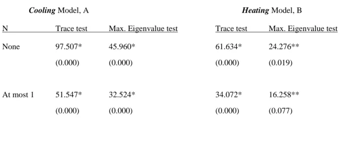
Having implemented a preliminary cointegration test by Johansen cointegration (Johansen, 1988) as indicated in Table 4 of the Appendix, the result of the ARDL further confirms evidence of cointegration. However, the ARDL estimates were subjected to further diagnostics to observe the validity of the results. In this case, both the Breusch-Godfrey serial correlation LM (Lagrange Multiplier) and the Breusch-Pagan-Godfrey heteroscedasticity tests were employed (see Table 3)
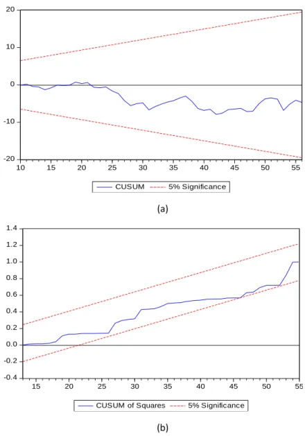
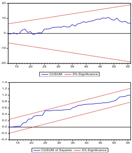
in addition to the CUSUM and the CUSUM square plots for the two models (see Figure 3 and 4). Importantly, the standard Granger causality test is employed as a robustness test. The test further illustrates the Granger causality among the investigated series as implied in Table 5. In addition to the robustness estimates, ecological footprint (efp) is further employed as a function of both the degree days (CDD and HDD) and the economic growth (measured by the GDP) by using the dynamic ARDL approach. The result of the estimate along with it diagnostic tests (including the Wald test) and the stability test (including the CUSUM and CUSUM of squares) are presented in Table 6 and Figure 5 of the Appendix respectively.
<Insert Table 4> <Insert Table 5> <Insert Table 6> <Figure 3> <Figure 4> <Figure 5>
4 Results and Discussion
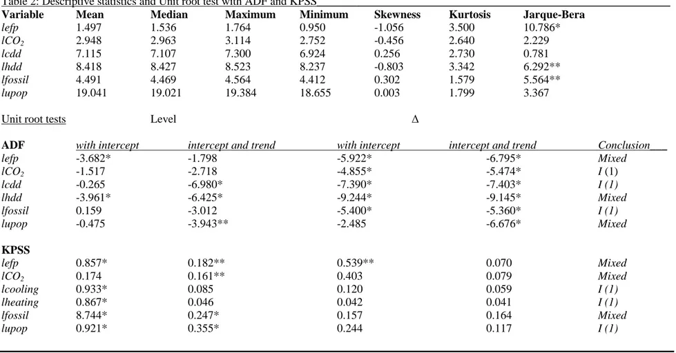
Given the common statistics presented in Table 2, there is less likelihood of a heteroskedastic concern in the observed datasets because of a relatively small difference between the maximum and minimum values. Also, except for the ecological footprint, the heating degree days and the non-renewable energy consumption, every other variable is normally distributed (according to the Jarque-Bera statistics). In the same vein, the ecological footprint, climate change, the heating degree days, and the renewable energy consumption are the only negatively skewed variables. the stationarity test result carried out prior to the main investigation reveals that the dataset
employed can be generally assumed as mixed order of integration. The reason for this is justified in the results of the ADF and KPSS employed for each of the variables where the variables are observed to be stationary at most at first difference (see Table 2). Hence, this pave way for the suitability of the ARDL approach.
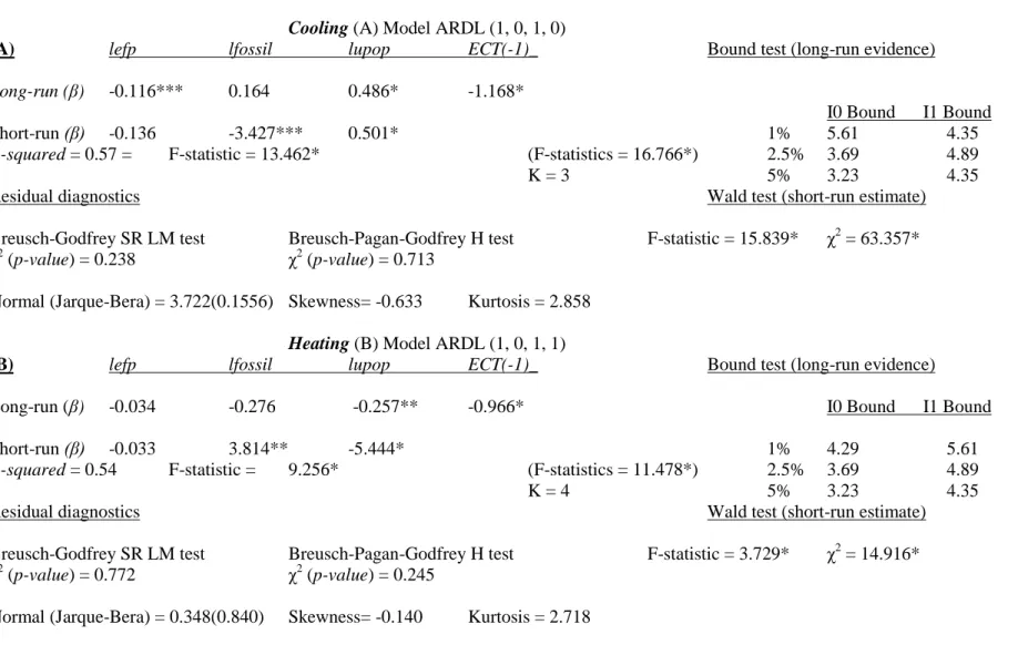
The cooling degree days
Furthermore, the ARDL approach employed reveals the roles fossil fuel energy consumption
fossil, ecological footprint (efp) and urban population (upop) on the cooling degree days (CDD)
of the United States (see Table 3). For CDD model, the result posits that the fossil fuel energy consumption increases the cooling degree days in the long-run in the United States. Although the impact of fossil on the CDD is observed to be positive and insignificant in the long-run, the short-run impact is negative and significant. As expected, the long-run impact translate that the consumption of the fossil fuel of energy which is largely responsible for pollutant emissions will significantly increases the length (in days) the United States experiences an atmospheric (outside) temperature that is above a certain level. Hence, a relatively long period of the hot weather (summer) is ensued such that increase the demand for more cooling technologies in the United States. This result outcome is supported by the report of the United States Global Change Research Program (USGCRP) that observed the increase in the cooling days as a result of high temperatures as against the decline in the cooling degree days until the 20th century (USGCRP, 2019). This is likely to be connected with the European case where the cooling degree days are reportedly on the high increase with the highest recorded in Southern Europe region. (European Environmental Agency, EEA, 2019). According to the EEA, while observing that the CDD has increased by 33% over the period 1950-2017 in the European region, the increase is projected to continue throughout the (21st) present century.
Moreover, the impact of the urban population (upop) and the ecological footprint (efp) on the cooling days in the United States. However, the upop and efp are observed to respectively exert positive and negative impacts on the CDD. The result implies that a percentage increase in the
upop and efp will expectedly cause the CCD to increase by 0.49 per cents and decrease by 0.12
per cents respectively. Importantly, it implies that as the urban population increases, more heat is expectedly generated thereby increasing the length of high temperature days (cooling degree days), thus causing higher demand for cooling needs and technologies. This result significantly louds the study of Otsuka and Goto (2018) and Spinoni et al (2018) that maintains that the impact of population on the CDD is positive. Similarly, this opinion was further strengthened by Shi et al (2018) by suggesting that population remains an important factor in both the heating and cooling dynamics. Shi et al (2018) considered the case of China for the investigation, therefore emphasizing that population distribution of the country is extremely uneven resulting from the climate condition, economic development, geographical location, and among others. Moreover, the concept of utilizing the urban population against the population of the rural dwellings in the context of climate change is strongly opined by Bird et al (2019).
Regarding the diagnostic investigation (see Table 3), the long-run evidence is corroborated by the statistical significance of the I0 and I1 bound which indicates that the F-statistics 16.766 > 5.61 of I1 at 1% significant level. Similarly, the short-run evidence (Wald test) present a significant F-statistic of 15.839 and chi-square of 63.357. In addition to the diagnostic evidence, the investigation has no drawback from neither serial correlation nor heteroscedasticity. Indicatively, the chi-squares (P-values) of the Breusch-Godfrey serial correlation LM (Lagrange Multiplier) test and the Breusch-Pagan-Godfrey heteroscedasticity test are respectively 0.238 and 0.713. Notwithstanding, a Normal distribution evidence from the Jarque-Bera statistic (3.722) in
Table 3 and both CUSUM and CUSUM of squares of Figure 3 (a & b respectively) are all desirable.
The heating degree days
In this case, the model is observed to adjust in a situation of short-run disequilibrium at a rate similar to the cooling degree days’ model. Unlike the CDD model earlier described the fossil fuel energy consumption exerts a negative and insignificant impact on the heating degree days in the long run (See Table 3). This expectedly suggests that the consumption fossil energy sources which is the main causative agent of climate change is responsible to cause less heating degree days, thus resulting to shorter cold or winter periods in the United States. In support of the fossil-HDD negative relationship observed in the current study, the United States Global Change Research Program (USGCRP) equally implies that the number of the HDD has continued to decline since about 1980 (USGCRP, 2019). This report is also corroborated by the record from the European counterpart which opined that the HDD has decreased by 6% between the periods 1950-2017 with the largest decrease recorded in the Northern European region and Italy.
Additionally, the impacts of ecological footprint and the urban population on the HDD are both observed to be negative in the long-run and short-run. Importantly, it implies that as the urban population increases, more heat is expectedly generated thereby reducing the length of low temperature days (heating degree days), thus causing lower demand for heating needs and technologies. The previous studies of Otsuka and Goto (2018) and Spinoni et al (2018) among other related investigations have also that there is a negative relationship between population and the heating degree days.
Similarly, the diagnostic results for the model are obviously desirable (See Table 3). Indicatively, the long-run evidence is corroborated by the statistical significance of the I0 and I1 bound which indicates that the F-statistics 11.48 > 5.61 of I1 at 1% significant level. This is in addition to the short-run evidence (Wald test) which presents a significant F-statistic of 3.73 and chi-square of 14.92. Also, tests suggest that the investigation is free form the concern of serial correlation and heteroscedasticity. This is because the chi-squares (P-values) of the Breusch-Godfrey serial correlation LM (Lagrange Multiplier) test and the Breusch-Pagan-Godfrey heteroscedasticity test are respectively presented as 0.77 and 0.25 in Table 3. Again, a Normal distribution evidence from the Jarque-Bera statistic (0.348) in Table 3 and both CUSUM and CUSUM of squares of Figure 4 (a & b respectively) adds to the desirability of the model specification.
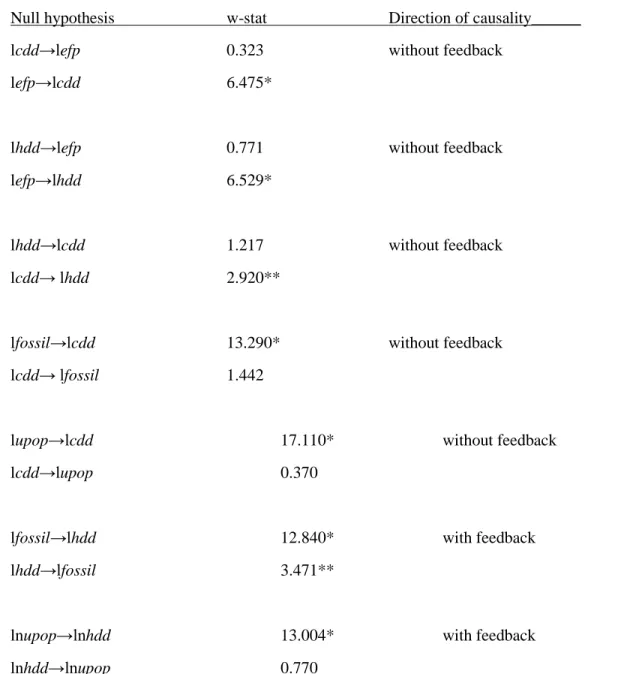
4.1 Robustness Evidence
Prior to employing the ARDL bound test approach, the Johansen cointegration (Johansen, 1988) test reveals at most one (1) cointegrating equation for both models (the CDD and HDD models) as indicated in Table 4 of the appendix. Similarly, the standard Granger causality as indicated in Table 5 of the appendix provides the directional relationship between the explanatory variables employed and the two dependent variables. In this case, the significant one-directional Granger causality relationship observed are: from ecological footprint to CDD, from ecological footprint to HDD, from fossil to CDD, and from upop to CDD and HDD. Whereas, the Granger causality from fossil to HDD is observed to be with feedback. In the context of the current study, the Granger causality relationships are desirable. Additionally, the dynamic ARDL estimate presents that the CDD and HDD exerts same (negative) direction of impacts on the ecological footprint (efp) in both long-run and short run (See Table 6). This result technically corroborates the earlier models (A and B) that expressed the relationship the variables. The GDP employed in this case
controls for other unobserved socio-economic factors. Lastly, the diagnostic Wald test (see Table 6) and the stability test (see Figure 5) further validates the earlier estimation.
5 Conclusions
In this study, the dynamic ARDL and the bound testing empirical techniques has been applied to investigate certain socio-economic and environmental activities that have potential effect on the cooling and heating days in the United States. For this reason, the two main primary source of pollutant emissions [(fossil fuel energy consumption (fossil)] and the ecological footprint (efp) are both employed as the economic and environmental variables while the urban population (upop) is utilized as a social indicator. Hence, the investigation revealed that the CDD and HDD are mostly affected by the aforementioned indicators over the period 1960 to 2015. While the impact of fossil on the CDD is (expectedly) positive (increasing the period of cooling degree days i.e. hotter or period), the fossil impact on the HDD is negative (reducing the length of heating degree days i.e less winter period) in both long-run and short-run. Similarly, the urban population (upop) and the ecological footprint (efp) indicators are observed to play significant role on the CDD and the HDD in the United States (Serrano, 2019; Tal, 2019). In this case, the upop is observed to exert positive impact on the CDD in both short-run and long run and a negative impact on the HDD in both the short-run and long run. Specifically, the United States urban population dynamics is observed to significantly determines the energy needs during each of the main climatic seasons (winter and summer period) (Moustris et al., 2015; Mastrucci et al., 2015). In line with the significant impacts the fossil fuel energy consumption, the ecological footprint, and the urban population on the heating and cooling degree days in the United States, feasible policy implications are proposed.
Considering the significant impact of the fossil fuel energy consumption on both the CDD and the HDD in the United States, and especially the adverse effects. a more robust energy efficient housing policy should be encouraged. This is simply because global building energy demand is a larger ratio of the global total energy consumption (United Nations Habitat, 2019). In this case, improved policy that provide guideline for housing and building constructions and especially for weather specifics and suitability is expected to be an efficient policy mechanism. Considering the importance of energy to the economy and the current stand of the United States government on climate change policy, this study posit that the government should have a policy re-think and continue to advance it energy portfolio diversification via environmental friendly mechanisms. In formulating policy vehicle for each of the seasonal dynamics (the CDD and HDD), the economic importance (benefits) of each of the climatic circumstances should be considered in designing the appropriate policy mechanism.
Lastly, future study could household decompositions of the socio-economic determinants of the cooling and heating degree days for the United States as well as other advance economy like China.
Reference
Alola, A. A. (2019a). The trilemma of trade, monetary and immigration policies in the United States: Accounting for environmental sustainability. Science of The Total Environment, 658, 260-267.
Alola, A. A. (2019b). Carbon emissions and the trilemma of trade policy, migration policy and health care in the US. Carbon Management, 10(2), 209-218.
Alola, A. A., Bekun, F. V., & Sarkodie, S. A. (2019). Dynamic impact of trade policy, economic growth, fertility rate, renewable and non-renewable energy consumption on ecological footprint in Europe. Science of The Total Environment, 685, 702-709.
Alola, A. A., Yalçiner, K., Alola, U. V., & Saint Akadiri, S. (2019). The role of renewable energy, immigration and real income in environmental sustainability target. Evidence from Europe largest states. Science of The Total Environment, 674, 307-315.
Auffhammer, M., & Mansur, E. T. (2014). Measuring climatic impacts on energy consumption: A review of the empirical literature. Energy Economics, 46, 522-530.
Central Intelligence Agency, CIA (2019). https://www.cia.gov/library/publications/the-world-factbook/fields/280.html#US. Retrieved 05 July 2019.
Bekun, F. V., Alola, A. A., & Sarkodie, S. A. (2019). Toward a sustainable environment: Nexus between CO2 emissions, resource rent, renewable and nonrenewable energy in 16-EU countries. Science of the Total Environment, 657, 1023-1029.
Bird, D. N., de Wit, R., Schwaiger, H. P., Andre, K., Beermann, M., & Žuvela-Aloise, M. (2019). Estimating the daily peak and annual total electricity demand for cooling in Vienna, Austria by 2050. Urban Climate, 28, 100452.
Collins, M., Knutti, R., Arblaster, J., Dufresne, J. L., Fichefet, T., Friedlingstein, P., ... & Shongwe, M. (2013). Long-term climate change: projections, commitments and irreversibility.
Day, T. (2006). Degree-days: theory and application. The Chartered Institution of Building
Services Engineers, London, 106.
Day, A. R., & Karayiannis, T. G. (1998). Degree-days: comparison of calculation methods. Building Services Engineering Research and Technology, 19(1), 7-13.
De Rosa, M., Bianco, V., Scarpa, F., & Tagliafico, L. A. (2015). Historical trends and current state of heating and cooling degree days in Italy. Energy conversion and management, 90, 323-335.
Dickey, D. A., & Fuller, W. A. (1979). Distribution of the estimators for autoregressive time series with a unit root. Journal of the American statistical association, 74(366a), 427-431.
Emir, F., & Bekun, F. V. (2019). Energy intensity, carbon emissions, renewable energy, and economic growth nexus: new insights from Romania. Energy & Environment, 30(3), 427-443.
Energy Information Administration (EIA, 2015). 2009 Residential Energy Consumption Survey/ https://www.eia.gov/consumption/residential/index.php. Retrieved 12 June 2019.
Energy Information Administration (EIA, 2019).
https://www.eia.gov/energyexplained/index.php?page=about_degree_days. Retrieved 12 June 2019.
European Environmental Agency, EEA (2019). Heating and cooling degree days. https://www.eea.europa.eu/data-and-maps/indicators/heating-degree-days-2/assessment. Retrieved 12 June 2019.
Fung, W. Y., Lam, K. S., Hung, W. T., Pang, S. W., & Lee, Y. L. (2006). Impact of urban temperature on energy consumption of Hong Kong. Energy, 31(14), 2623-2637.
Global Change Research Program, USGCRP (2019).
https://www.globalchange.gov/browse/indicators/indicator-heating-and-cooling-degree-days. Retrieved 05 July 2019.
Johansen, S. (1988). Statistical analysis of cointegration vectors. Journal of economic dynamics
and control, 12(2-3), 231-254.
Karl, T. R., Melillo, J. M., Peterson, T. C., & Hassol, S. J. (Eds.). (2009). Global climate change
impacts in the United States. Cambridge University Press.
Kwiatkowski, D., Phillips, P. C., Schmidt, P., & Shin, Y. (1992). Testing the null hypothesis of stationarity against the alternative of a unit root: How sure are we that economic time series have a unit root? Journal of Econometrics, 54(1-3), 159-178. doi.org/10.1016/0304-4076 (92)90104-Y.
Labriet, M., Joshi, S. R., Vielle, M., Holden, P. B., Edwards, N. R., Kanudia, A., & Babonneau, F. (2015). Worldwide impacts of climate change on energy for heating and cooling.
Mitigation and Adaptation Strategies for Global Change, 20(7), 1111-1136.
Le Comte, D. M., & Warren, H. E. (1981). Modeling the impact of summer temperatures on national electricity consumption. Journal of Applied Meteorology, 20(12), 1415-1419.
Mastrucci, A., Byes, E., Pachauri, S., & Rao, N. D. (2019). Improving the SDG energy poverty targets: Residential cooling needs in the Global South. Energy and Buildings, 186,
405-415.
Melillo, J. M. (2014). Climate change impacts in the United States: the third national climate
assessment. Government Printing Office.
Mourshed, M. (2012). Relationship between annual mean temperature and degree-days. Energy
and buildings, 54, 418-425.
Moustris, K. P., Nastos, P. T., Bartzokas, A., Larissi, I. K., Zacharia, P. T., & Paliatsos, A. G. (2015). Energy consumption based on heating/cooling degree days within the urban
environment of Athens, Greece. Theoretical and Applied Climatology, 122(3-4), 517-529.
Otsuka, A., & Goto, M. (2018). Regional determinants of energy intensity in Japan: the impact of population density. Asia-Pacific Journal of Regional Science, 2(2), 257-278.
Pesaran, M. H., Shin, Y., & Smith, R. J. (2001). Bounds testing approaches to the analysis of level relationships. Journal of applied econometrics, 16(3), 289-326.
Quayle, R. G., & Diaz, H. F. (1980). Heating degree day data applied to residential heating energy consumption. Journal of Applied Meteorology, 19(3), 241-246.
Rasmussen, D. J., Meinshausen, M., & Kopp, R. E. (2016). Probability-weighted ensembles of US county-level climate projections for climate risk analysis. Journal of Applied
Meteorology and Climatology, 55(10), 2301-2322.
Saint Akadiri, S., Alola, A. A., & Akadiri, A. C. (2019). The role of globalization, real income, tourism in environmental sustainability target. Evidence from Turkey. Science of The
Total Environment.
Saint Akadiri, S., Alola, A. A., Akadiri, A. C., & Alola, U. V. (2019). Renewable energy consumption in EU-28 countries: policy toward pollution mitigation and economic sustainability. Energy Policy, 132, 803-810.
Sailor, D. J., & Muñoz, J. R. (1997). Sensitivity of electricity and natural gas consumption to climate in the USA—methodology and results for eight states. Energy, 22(10), 987-998.
Serrano, S., Ürge-Vorsatz, D., Barreneche, C., Palacios, A., & Cabeza, L. F. (2017). Heating and cooling energy trends and drivers in Europe. Energy, 119, 425-434.
Shi, Y., Zhang, D. F., Xu, Y., & Zhou, B. T. (2018). Changes of heating and cooling degree days over China in response to global warming of 1.5° C, 2° C, 3° C and 4° C. Advances in
Climate Change Research, 9(3), 192-200.
Solomon, S., Qin, D., Manning, M., Chen, Z., Marquis, M., Averyt, K., ... & Miller, H. (2007). IPCC fourth assessment report (AR4). Climate change.
Spinoni, J., Vogt, J. V., Barbosa, P., Dosio, A., McCormick, N., Bigano, A., & Füssel, H. M. (2018). Changes of heating and cooling degree‐ days in Europe from 1981 to 2100.
International Journal of Climatology, 38, e191-e208.
Tal, A. (2019). Climate change's impact on Lake Kinneret: Letting the data tell the story. The
Science of the total environment.
The United States Environmental Protection Agency (US EPA, 2019). https://www.epa.gov/climate-indicators/climate-change-indicators-heating-and-cooling-degree-days. Retrieved 12 June 2019.
United Nations Habitat (2019). Energy. https://unhabitat.org/urban-themes/energy/. Retrieved 09 July, 2019.
Valor, E., Meneu, V., & Caselles, V. (2001). Daily air temperature and electricity load in Spain. Journal of applied Meteorology, 40(8), 1413-1421.
Wilbanks, T., Bhatt, V., Bilello, D., Bull, S., Ekmann, J., Horak, W., ... & Scott, M. J. (2008). Effects of climate change on energy production and use in the United States. US Department
Wang, H., & Chen, Q. (2014). Impact of climate change heating and cooling energy use in buildings in the United States. Energy and Buildings, 82, 428-436.
Wang, X., Chen, D., & Ren, Z. (2010). Assessment of climate change impact on residential building heating and cooling energy requirement in Australia. Building and
Environment, 45(7), 1663-1682.
Source: The United States Environmental Protection Agency (US EPA, 2019). https://www.epa.gov/climate-indicators/climate-change-indicators-heating-and-cooling-degree-days.
Figure 1: A visual observation of the trend of the cooling and heating degree days, the ecological footprint (efp), and the carbon dioxide (CO2) emissions in the United States over the period 1960-2015.
0 1 2 3 4 5 6 7 8 1960 1962 1964 1966 1968 1970 1972 1974 1976 1978 1980 1982 1984 1986 1988 1990 1992 1994 1996 1998 2000 2002 2004 2006 2008 2010 2012 2014
A line plot of the logarithmic of cooling and heating degree days, ecological footprint, and the CO2 emissions in the United States
Table 1: Variable description and measurement unit____________________________________ Indicator Name Abbreviation Measurement Scale Source______
Cooling Degree Days CDD Degree days USEPA
Heating Degree Days HDD Degree days USEPA
Fossil Energy Consumption FOSSIL % of total energy WDI
Urban Population UPOP Birth woman total term WDI
Ecological Footprint EFP Global hectares (GHA) EFP
Gross Domestic Product GDP Constant 2010 US Dollars WDI
______________________________________________________________________________
Source: Authors’ computation.
Note: US EPA2, US EIA3 and WDI4 represents the United States Environmental Protection Agency, United States Energy Information Administration, and World Development Indicator respectively.
2 https://www.epa.gov/climate-indicators/climate-change-indicators-heating-and-cooling-degree-days 3https://www.eia.gov/totalenergy/data/browser/index.php?tbl=T10.01#/?f=M&start=200001
4https://data.worldbank.org/indicator. The more detail information on the description of the variables are available at
Table 2: Descriptive statistics and Unit root test with ADF and KPSS______________________________________________________________
Variable Mean Median Maximum Minimum Skewness Kurtosis Jarque-Bera
lefp 1.497 1.536 1.764 0.950 -1.056 3.500 10.786* lCO2 2.948 2.963 3.114 2.752 -0.456 2.640 2.229 lcdd 7.115 7.107 7.300 6.924 0.256 2.730 0.781 lhdd 8.418 8.427 8.523 8.237 -0.803 3.342 6.292** lfossil 4.491 4.469 4.564 4.412 0.302 1.579 5.564** lupop 19.041 19.021 19.384 18.655 0.003 1.799 3.367
Unit root tests Level Δ
ADF with intercept intercept and trend with intercept intercept and trend Conclusion___
lefp -3.682* -1.798 -5.922* -6.795* Mixed lCO2 -1.517 -2.718 -4.855* -5.474* I (1) lcdd -0.265 -6.980* -7.390* -7.403* I (1) lhdd -3.961* -6.425* -9.244* -9.145* Mixed lfossil 0.159 -3.012 -5.400* -5.360* I (1) lupop -0.475 -3.943** -2.485 -6.676* Mixed KPSS lefp 0.857* 0.182** 0.539** 0.070 Mixed lCO2 0.174 0.161** 0.403 0.079 Mixed lcooling 0.933* 0.085 0.120 0.059 I (1) lheating 0.867* 0.046 0.042 0.041 I (1) lfossil 8.744* 0.247* 0.157 0.164 Mixed lupop 0.921* 0.355* 0.244 0.117 I (1)
Note: Level and Δ respectively indicates estimates at the level and the first difference with lag selection by SIC (lag=4) for the ADF (Augmented Dickey-Fuller) and KPSS (using the Bartlett Kernel of Andrews automatic Bandwidth) unit root tests. *, ** and *** are the 1%, 5% and 10% statistical significance levels. Number of observation is 56.
Table 3: Dynamic ARDL-Bound Test_______________________________________________________________________________________
Cooling (A) Model ARDL (1, 0, 1, 0)
(A) lefp lfossil lupop ECT(-1)_ Bound test (long-run evidence)
Long-run (β) -0.116*** 0.164 0.486* -1.168*
I0 Bound I1 Bound
Short-run (β) -0.136 -3.427*** 0.501* 1% 5.61 4.35
R-squared = 0.57 = F-statistic = 13.462* (F-statistics = 16.766*) 2.5% 3.69 4.89
K = 3 5% 3.23 4.35
Residual diagnostics Wald test (short-run estimate)
Breusch-Godfrey SR LM test Breusch-Pagan-Godfrey H test F-statistic = 15.839* χ2 = 63.357* χ2
(p-value) = 0.238 χ2 (p-value) = 0.713
Normal (Jarque-Bera) = 3.722(0.1556) Skewness= -0.633 Kurtosis = 2.858
Heating (B) Model ARDL (1, 0, 1, 1)
(B) lefp lfossil lupop ECT(-1)_ Bound test (long-run evidence)
Long-run (β) -0.034 -0.276 -0.257** -0.966* I0 Bound I1 Bound
Short-run (β) -0.033 3.814** -5.444* 1% 4.29 5.61
R-squared = 0.54 F-statistic = 9.256* (F-statistics = 11.478*) 2.5% 3.69 4.89
K = 4 5% 3.23 4.35
Residual diagnostics Wald test (short-run estimate)
Breusch-Godfrey SR LM test Breusch-Pagan-Godfrey H test F-statistic = 3.729* χ2 = 14.916* χ2
(p-value) = 0.772 χ2 (p-value) = 0.245
Normal (Jarque-Bera) = 0.348(0.840) Skewness= -0.140 Kurtosis = 2.718
______________________________________________________________________________________________________________________
Note: Autoregressive Distributed Lad (ARDL) model employed are: A is (1, 0, 1, 0) and B is (1, 0, 1, 1), the p-value is the probability value and ECT is the Error
Correction Term also known as the adjustment parameter. The I0 and I1 are lower and upper bound of the bound test respectively, β is the estimate coefficient, χ2 is the Chi-square, SR LM is Serial correlation Lagrange Multiplier and H is heteroscedasticity. A and B are the models for the cooling and heating degree days respectively.
-30 -20 -10 0 10 20 30 10 15 20 25 30 35 40 45 50 55 CUSUM 5% Significance (a) -0.4 -0.2 0.0 0.2 0.4 0.6 0.8 1.0 1.2 1.4 10 15 20 25 30 35 40 45 50 55 CUSUM of Squares 5% Significance
(b)
Figure 3: The CUSUM (a) and CUSUM of Squares (b) of stability test respectively for the cooling model A (CDD).
-20 -10 0 10 20 10 15 20 25 30 35 40 45 50 55 CUSUM 5% Significance (a) -0.4 -0.2 0.0 0.2 0.4 0.6 0.8 1.0 1.2 1.4 15 20 25 30 35 40 45 50 55 CUSUM of Squares 5% Significance
(b)
Figure 4: The CUSUM (a) and CUSUM of Squares (b) of stability test respectively for the heating model B (HDD).
Appendix
Table 4: Johansen Cointegration test_______________________________________________________
Cooling Model, A Heating Model, B
N Trace test Max. Eigenvalue test Trace test Max. Eigenvalue test
None 97.507* 45.960* 61.634* 24.276**
(0.000) (0.000) (0.000) (0.019)
At most 1 51.547* 32.524* 34.072* 16.258**
(0.000) (0.000) (0.000) (0.077)
_____________________________________________________________________________________
Note: The estimate adopts the SIC (maximum lag = 4). * and ** indicate statistical significance level of 1% and 5%
Table 5: Standard Granger causality results ___________________________________________
Null hypothesis w-stat Direction of causality______
lcdd→lefp 0.323 without feedback
lefp→lcdd 6.475*
lhdd→lefp 0.771 without feedback
lefp→lhdd 6.529*
lhdd→lcdd 1.217 without feedback
lcdd→ lhdd 2.920**
lfossil→lcdd 13.290* without feedback
lcdd→ lfossil 1.442
lupop→lcdd 17.110* without feedback
lcdd→lupop 0.370
lfossil→lhdd 12.840* with feedback
lhdd→lfossil 3.471**
lnupop→lnhdd 13.004* with feedback
lnhdd→lnupop 0.770
Note: *, ** and *** are the 1%, 5% and 10% statistical significance levels. ln is the natural logarithmic values of the
Table 6: Dynamic ARDL estimate with lefp (Robustness Output) ______________________________
lcdd lhdd lgdp ECT (-1) ____
Long-run (β) -1.433*** -0.639 0.224*
Short-run (β) -0.204* -0.091 0.979* -0.243**
R-squared = 0.98 F-statistic = 315.603* Wald Test (short-run estimate)
F-statistic = 8.637* χ2 = 34.546*
Note : The lefp, lcooling, lheating, and lgdp are the logarithmic values of the ecological footprint, cooling days,
heating days, and Gross Domestic Product respectively. ARDL is the Autoregressive Distributed Lag while the ECT is the Error Correction Term. Also, β is the estimate coefficient, χ2 is the Chi-square,
-20 -10 0 10 20 15 20 25 30 35 40 45 50 55 CUSUM 5% Significance -0.4 -0.2 0.0 0.2 0.4 0.6 0.8 1.0 1.2 1.4 15 20 25 30 35 40 45 50 55
CUSUM of Squares 5% Significance
Figure 5: The CUSUM (top) and CUSUM of Squares (beneath) of stability