Business cycle modelling - The case of mergers and acquisitions

ISSN 1993-8233 ©2012 Academic Journals

Full Length Research Paper

Business cycle modelling - The case of mergers and

acquisitions

Yıldız Guzey

1

* and Ozlem Tasseven

2

1

Department of International Trade and Finance, Izmir University, Uckuyular, Izmir, Turkey.

2

Department of Economics and Finance, Faculty of Economics and Business Administration, Dogus University, Acıbadem, Kadıköy, 34722 İstanbul, Turkey.

Accepted 15 June, 2012

Business cycle models involve exploiting movements of the economy to gain competitive advantage over rivals. Business cycles are applicable to mergers and acquisitions (M&A) which occur in waves. Econometricians have attempted to model these waves. The paper demonstrates that, with respect to each of several major stylized facts about business cycles, the seasonal cycle displays the same characteristics as the business cycle. Therefore the patterns in merger and acquisitions measured as merger waves could be investigated using seasonality models. Using a modified seasonal unit root procedure we model the cyclical behaviour in the quarterly M&A data from 2000 to 2010 for Turkey. Our analysis is based on the methodology developed by Hylleberg, Engle, Granger and Yoo (HEGY procedure). Based upon an empirical analysis of the merger and acquisition variables, our results indicate that seasonal unit roots appear to deal value, number of deals with known value variables when possible structural changes in one or more seasons during the 2001 and 2008 crisis years have been taken into account.

Key words: Merger and acquisitions, Turkish economy, Hylleberg, Engle, Granger and Yoo (HEGY) seasonal

unit root test, deterministic seasonality, structural breaks.

INTRODUCTION

Even though the number of mergers and acquisitions is associated with the effect of globalization, merger waves have long been an area of interest for economists. Even if the basic elements of economic shocks, the reasons why and how companies respond to shocks cannot be fully explained, related literature attributes merger waves to economic shocks. Researchers state that understanding the drivers of M and As means understanding their cyclical and seasonal nature (Golbe and White, 1993; Gregoria and Renneboog, 2007). Ghysels (1991) noted the relationship between business cycle and seasonal cycle and pointed out the difference of macroeconomic time series and seasonal patterns of recessions and expansions. Canova and Ghysels (1994)

*Corresponding author. E-mail: otasseven@dogus.edu.tr.

proved that structural instability shows constant and slow changing characteristics together with business cycle fluctuations like seasonal cycles.

There are authoritative studies on the relationship between M and As, macroeconomic indicators and business cycles in general. The methods, data utilized, and the standing point differ and findings vary greatly. In general, “cycles” are described as “time segments with specific distinctive characteristics that follow each other in a specific period” (Barsky and Miron, 1989). In general, crisis and shock are known as disturbance that occurred due to a sudden unexpected change (Ferguson, 1969). Merger waves emerge as companies react to economic shocks (Jensen, 1986; Mitchell and Mulherin, 1996). Harford (2003) presented the effects of economic cycles on the emergence of mergers and acquisitions, and pointed out that this relationship adds a cyclical characteristic to mergers, but that correlation might be

related to different stages of the business cycles. Nelson (1959) pointed out the presence of a sensitive and chronic relationship between M and As and economic cycles.

Most empirical studies demonstrate that merger and acquisition cycles are associated with economic cycles. Melicher et al. (1983) and Markham (1955) found a strong relationship between merger activities, industrial activities and the economic cycles based on the quarterly M and A data of the Federal Trade Commission published in 1947 to 1977. Some research results demonstrate that M and A activity has a negative correlation with recessions and also that this activity is more than a quarter cycle ahead of the recession (Melicher et al., 1983).

Neoclassical theory assumed that economic fluctuations or instability within the economic system will stabilize on their own. According to this view, waves are cyclical; and it is important to emphasize that, a cycle is not a depression in neoclassical theory (Golbe and White, 1993). System of regular mild fluctuations is inherent, shrinkages and expansions are parts of the ordinary economic cycle. On the contrary, Blanchard (1987) argued that severe and long-term expansions and shrinkages occur due to external factors.

Gort (1969) stated that economic dispersals and waves cause sectors to restructure. Jovanovic and Rousseau (2001) concurred with Gort’s (1969) opinion and developed the Q Theory of Takeovers in which it claimed that economic and technological shocks give companies an opportunity for growth. According to Neoclassical models, takeover clustering by industry and by country merger waves results from the firms’ responses to the actions of their competitors. Another factor that transforms merger movements into waves in sectors is the companies mimicking of each other (Persons and Warther, 1997; Mitchell and Mulherin, 1996).

It is observed that merger density increases and follows a waved behavior in certain periods and regions in parallel with the development of capitalist economies. Six important merger waves can be identified, starting from the 1890s to the present; these were seen in the 1890s, 1920s, 1960s, 1980s and 1990s. The sixth merger wave began toward the end of 2003 and is ongoing (Gregoriou and Renneboog, 2007). In fact, in 2006, the worldwide M and A deal total was US$4 trillion, beating the previous record of US$3.3 trillion set in 2000. US and European firms accounted for almost 80% of these deals (Zephyr, 2010).

In many economic variables, the size of the seasonal cycle clearly dwarfs the business cycle. Accordingly, we investigate the cyclical behavior in merger and acquisition (M and A) data for Turkey. The objective of this paper is to model the seasonal cycle using the modified seasonal unit root process. We extend the Hylleberg et al. (1990), Hylleberg, Engle, Granger and Yoo (HEGY) seasonal unit root testing procedure by allowing for the seasonal mean

shifts in more than one year while considering also exogenous break points. For this purpose, we have attempted to analyse innovational outlier tests to seasonal unit roots. In this paper, the structural break dates are taken as exogeneous, namely the financial crises in 2001 and 2008.

The work is structured as follows: firstly it proposes the influences of merger and acquisitions and business cycles. Secondly, we discuss the relationship between merger waves and seasonality. Then seasonal unit root procedures and our modified test procedure are presented briefly. An empirical analysis of merger and acquisition variables using the HEGY testing procedures is conducted for the Turkish economy. Finally we summarize the results.

MERGER WAVES AND SEASONALITY

The fact that merger activity is cyclical is clearly related with the characteristics of time series: in particular the seasonality component. The underlying pattern in the M&A data can be characterized by the shifts in the seasonal pattern of time series. The celebrated definition of seasonality by Hylleberg (1992) stated that seasonal cycles are rooted in various sources, among which the climate, cultural traditions and technology play a key role. The increasing trade, division of labor and production processes and integration in various fields in companies would motivate a tendency toward a convergence of seasonal patterns, particularly as the relationship of business cycles and seasonal cycles has been demonstrated empirically as well as on theoretical grounds (Miron, 1996) for the former and Ghysels (1988) for the latter.

The study of seasonal properties of economic time series has been the subject of considerable research in the last decade (Hylleberg et al., 1990; Miron, 1994). The finding of these studies is that, in addition to being nonstationary at the zero frequency, many seasonal time series have seasonal unit roots at other frequencies as well. It has been found that some variables show a deterministic seasonal pattern, while others display seasonal movements that change slowly over time. Most of the literature has found that the seasonality in time series is best described by a deterministic process or one with stochastic trends at seasonal frequencies.

It is very important to know which periods business cycles and seasonal factors affect business cycles. Seasonality can create different effects on business cycles on different sectors in different periods. Warner and Barsky (1995) claimed that in the United States of America, retail prices are lower on holidays and weekends. Cooper and Haltiwanger (1993) stated that seasonality in the automobile sector is remarkable and studied the important effects of new models on sales in the sector. They demonstrated that gross seasonality in

the auto industry is driven by supply-side effects. Einav (2007) stated that tourism, apparel and airlines are sectors where seasonality effects are heavily observed and the emerging seasonal effects present a serious relationship between prices, sales and demand.

Using the National Bureau of Economic Research (NBER) business cycle chronology, Ghysels (1991) found that the seasonal patterns in a number of U.S. macroeconomic time series differ between recessions and expansions. The general tests in Canova and Ghysels (1994) also provide evidence of structural instability in models that treat seasonality as constant or slow changing, with the instability often associated with business cycle fluctuations. Building on these more structural frameworks, Beaulieu et al. (1992) showed how firm-level production functions can transform independent seasonal and nonseasonal variation into interactions between the business cycle and seasonality in macroeconomic aggregates. Beaulieu et al. (1992) used these arguments to explain the strong positive correlations between the seasonal and nonseasonal variation in retail sales, employment and numerous other time series that they find across a variety of countries and industries.

Despite some major advances in the study of seasonality from an economic as well as from an econometric perspective (Hylleberg, 1992; Ghysels and Osborn, 2001), it was felt that this aspect of economic behaviour does not yet catch the attention it would deserve.

Seasonal unit root tests procedures

A large body of seasonal unit root tests has been proposed to test for the appropriateness of the filters

∆₁(first differencing) and ∆_s(seasonal differencing) for

removing non-seasonal and seasonal stochastic trends in the time series data. In this sense, the most important seasonal unit root tests can be attributed to the estimation procedures developed by Dickey et al. (1984), Osborn et al. (1988), HEGY (1990) and Canova and Hansen (1995). Among all these HEGY (1990) is the one widely used to test for seasonal and non-seasonal unit roots in a univariate series. This can be shown based on the following auxiliary regression:

φ(L)y4,t = µt + π1y1,t-1 + π2y2,t-1+ π3y3,t-2 + π4y3,t-1+ εt (1)

where φ(L) is an AR polynomial of order p-4 and εt is a

normally and independently distributed (i.i.d) error term with the assumption of zero mean and constant variance. µt is defined as: µt = t 3 1 t st s

D

β

δ

α

+

∑

+

= (2) where: y1,t = (1+L+L2+L3) yt y2,t = -(1-L)(1+L2) yt y3,t = -(1-L 2 ) yt y4,t = (1-L 4 ) yt

The unit root 1 is called the non-seasonal unit root, whereas unit roots -1, +i and –i are called seasonal unit roots (Hylleberg et al., 1990). Deterministic components which include an intercept (α), three seasonal dummies (Dst) and a time trend (βt) are also included in Equation 1

that can be estimated by ordinary least squares (OLS) estimators. The relevant null and alternative hypotheses to be tested can be given as follows:

[H0: π1 = 0,] [H1: π1 <0]; (3)

[H0: π2 = 0], [H1: π2 <0]; (4)

[H0: π3 = 0], [H0: π4 = 0], [H1]:[ π3≠ 0 or π4≠ 0] (5)

The HEGY test involves the use of the t-test for the first two hypotheses and an F-test for the third hypothesis. Non-rejection of the first hypothesis would mean a unit root at the zero frequency or a non-seasonal unit root in the series. Non-rejection of the second hypothesis would show that there exists seasonal unit root at the semi-annual frequency. Finally, if the third hypothesis is not rejected we can infer that there exists a seasonal unit root at the annual frequency. These null hypotheses are tested separately. Critical values for the one sided t-tests for π1 toπ4 (F34) have been given in HEGY (1990).

SEASONAL UNIT ROOT TESTS WITH SEASONAL MEAN SHIFTS IN ONE YEAR

Perron (1989) argued that structural changes to the trend function can be viewed as some kind of big shocks or infrequent events that have permanent effects on the level of the series. Franses and Vogelsang (1995) tried to consider testing for the seasonal unit roots in the presence of changing seasonal means with exogenous break point. It is assumed that there is a single break which occurs at time TB’ where 1<TB’<T. The additive outlier model for quarterly time series under the null hypothesis of one non-seasonal unit root and three seasonal unit roots can be written as follows:

yt =

∑

₌

4 1

s

κ

s

D(TB'

)

s,t + yt-4 + wt, (6) where:

D(TB’)1,t = 1 if t = TB1+ 1 (and zero elsewhere)

D(TB’)2,t = 1 if t = TB1+ 2 (and zero elsewhere)

D(TB’)4,t = 1 if t = TB1+ 4 (and zero elsewhere)

wt represents a stationary and invertible ARMA(p,q)

process. Under the alternative hypothesis, the series yt

does not contain any of these unit roots and can be written as follows: yt =

∑

₌ 4 1 s

µ

s

D

s,t +

∑

= 4 1 s

κ

s

DU

s,t + vt (7) where vt is a stationary and invertible ARMA(p+4,q)

process and Ds,t the seasonal dummies for the entire

sample for:

DU1,t = 1 if t >TB’ and tmod=1, (and zero elsewhere)

DU2,t = 1 if t >TB’ and tmod=2, (and zero elsewhere)

DU3,t = 1 if t >TB’ and tmod=3, (and zero elsewhere)

DU4,t = 1 if t >TB’ and tmod=4, (and zero elsewhere)

DUs,t = 1 (t > TB’)Ds,t where1(.) is the indicator function

and tmod shows the corresponding season of this function. DUs,t can be defined asseasonaldummies that

only take non-zero values in the corresponding seasons when t > TB’. DU terms allow for the break under the alternative hypothesis. Franses and Vogelsang (1995) present asymptotic and small sample critical values for additive and innovative outlier models for known and estimated break points.

MATERIALS AND METHODS

Modified HEGY test procedure for testing seasonal unit roots in the presence of seasonal mean shifts in two years

In this area, we extend our analysis by examining the presence of two breaks for seasonal unit roots. For this purpose the HEGY test procedure is modified by adding the structural break dummy variables which become effective only at time TB1 and TB2, where

TB1 = λ1T with 0< λ1<1 and TB2 = λ2T with 0< λ2<1 and

1<TB1<TB2<T. The model for quarterly time series under the null

hypothesis of one non-seasonal unit root and three seasonal unit roots is written as follows:

yt = yt-4 + εt (8)

where εt is the iid error term. Under the alternative hypothesis, the

series yt does not contain any of these unit roots and can be written

as follows: yt =

∑

= 4 1 s

µ

s

D

s,t+ ut (9) where ut is again iid and Ds are seasonal dummies for the entire

sample. The relevant data generation process used in the analyses is given as follows:

∆4yt = εt (10)

where εt ~ iidN (0,1). The auxiliary regression used in our model is:

φ(B)y4,t = µt + π1y1,t-1 + π2y2,t-1 + π3y3,t-2 + π4y3,t-1 +

∑

4s₌1

θ

s

D(TB

1

)

s,t +

∑

= 4 1 s

γ

s

D(TB

2

)

s

,

t +

∑

4₌ 1 s

δ

s

DU(TB

1

)

s

,

t+

∑

= 4 1 s

λ

s

DU(TB

2

)

s

,

t+ εt (11) where εt is a stationary and invertible ARMA(p+4,q) process, the

D(TB1)s,t are single observation dummy variables with the following

properties:

D(TB1)1,t = 1 if t = TB1+ 1 (and zero elsewhere)

D(TB1)2,t = 1 if t = TB1+ 2 (and zero elsewhere)

D(TB1)3,t = 1 if t = TB1+ 3 (and zero elsewhere)

D(TB1)4,t = 1 if t = TB1+ 4 (and zero elsewhere)

D(TB2)s,t can also be considered as single observation dummy

variables:

D(TB2)1,t = 1 if t = TB2+ 1 (and zero elsewhere)

D(TB2)2,t = 1 if t = TB2+ 2 (and zero elsewhere)

D(TB2)3,t = 1 if t = TB2+ 3 (and zero elsewhere)

D(TB2)4,t = 1 if t = TB2+ 4 (and zero elsewhere)

where DU(TB1)s,t are composed to allow for the first structural break

under the alternative hypothesis:

DU(TB1)1,t = 1 if t >TB1 and tmod=1 (and zero elsewhere)

DU(TB1)2,t = 1 if t >TB1 and tmod=2 (and zero elsewhere)

DU(TB1)3,t = 1 if t >TB1 and tmod=3 (and zero elsewhere)

DU(TB1)4,t = 1 if t >TB1 and tmod=4 (and zero elsewhere)

and DU(TB2)s,t are composed to allow for the second structural

break under the alternative hypothesis:

DU(TB2)1,t = 1 if t >TB2 and tmod=1 (and zero elsewhere)

DU(TB2)2,t = 1 if t >TB2 and tmod=2 (and zero elsewhere)

DU(TB2)3,t = 1 if t >TB2 and tmod=3 (and zero elsewhere)

DU(TB2)4,t = 1 if t >TB2 and tmod=4 (and zero elsewhere)

DU(TB1)s,t = 1 (t>TB1)Ds,t and DU(TB2)s,t = 1 (t>TB2)Ds,t where1(.) is

the indicator function and tmod shows the corresponding season of this function. DU(TB1)s,t can be defined asseasonaldummies that

only take non-zero values in the corresponding seasons when t > TB1 and DU(TB2)s,t can be defined asseasonal dummies that only

take non-zero values in the corresponding seasons when t > TB2.

The auxiliary regression is augmented by the lagged values of the dependent variable. The lag selection method involves testing for the significance of the coefficient of ∆_{4yt-k using a 10% significance} level two sided t-test which is asymptotically distributed N(0, 1).

Design of Monte Carlo simulation

In the Monte Carlo investigation the critical values of the HEGY test in the presence of two structural breaks are generated in a GAUSS programme version 4. The critical values for the small sample distributions are displayed for the following different combinations of deterministic terms in the auxiliary regression as in HEGY (1990) and Franses and Hobijn (1997): 1) no intercept, seasonal dummy and trend, 2) intercept, no seasonal dummy and no trend, 3) intercept, seasonal dummy and no trend, 4) intercept, no seasonal dummy and trend, 5) intercept, seasonal dummy and trend.

These cases refer to different model specifications depending on which deterministic terms are used. The critical values for the one– sided t-test for π1,critical values for the t-test for π2, the F-test

statistics for {π3, π4}, {π2, π3, π4} and {π1, π2, π3, π4} are generated.

procedure for testing seasonal unit roots considering break fractions λ1 =0.1, 0.3, 0.5, 0.7, 0.9 and λ2 = 0.2, 0.4, 0.6, 0.8 in a

sample size of 40. The GAUSS code used in generating the critical values and test statistics are available upon request.

Application

In this area the modified test procedure for testing seasonal unit roots in the presence of possible shifts in the seasonal means is considered by analysing the variables related with merger and acquisitions, which are the number of deals, number of deals with known values and the deal value of mergers and acquisitions in Turkey for the 2001:1 to 2010:4 period. Our data set includes the period in which two financial crises in 2001 and 2008 took place.

RESULTS

Original and modified HEGY test results

In this area we have tried to estimate the original HEGY test using auxiliary regression (1), where the possible presence of seasonal mean shifts is neglected, and the modified HEGY test for testing seasonal unit roots in the presence of possible shifts in the seasonal means in two years. The empirical results of the original HEGY and the modified HEGY seasonal unit root tests are discussed for each variable. While comparing these two HEGY test results it should be mentioned that the original HEGY test can be considered more powerful when a series does not actually have seasonal mean shifts.

The auxiliary regression (11) for testing seasonal unit roots in the presence of breaks is used for hypothesis testing. Since there is a priori knowledge of the timing of possible break dates, we calculate λ1 and λ2

corresponding to the exogenous break dates. Assuming that the mean shifts have occurred in the first quarter of 2001 because of the massive economic crisis experienced by the Turkish economy, we set TB1 in (11) at 2001:1 corresponding to λ1=0.125. The second major

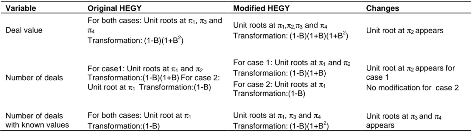
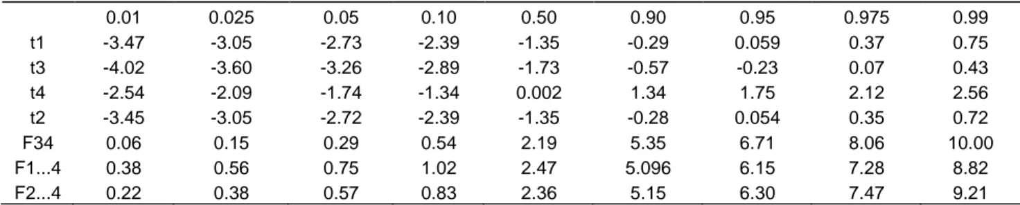
change occurs at 2008: 3 because of a massive financial crisis, therefore we set λ₂ =0.875. By looking at the test results obtained from original HEGY and modified HEGY test procedures given in Table 1 give in the Appendix, it can be seen that there are clearly some variations in the outcomes. The test results vary based on whether the deterministic terms such as seasonal dummy variables and the trend are included in the model and whether 5 or 1% critical value is used for testing. The critical values are given in Table 2 give in the Appendix. The original HEGY regressions for the variables of interest include constant, three seasonal dummy variables and trend in case 1 and constant and three seasonal dummy variables in case 2. The results of the original HEGY test for the deal value show that there are non-seasonal and seasonal unit roots at annual frequency. For the deal value series, when the structural breaks at 2001 and 2008 are allowed in the analysis, the deal value appears to have a seasonal unit root at the bi-annual frequency.

The results of the original HEGY test for the number of deals show that there is non-seasonal unit root at zero frequency and seasonal unit root bi-annual frequency for case 1. However, for case 2 only unit root at the nonzero frequency is found to exist. The empirical results suggest that the results of the original HEGY test for the number of deals data are robust for the structural breaks at 2001 and 2008 for case 2. For case 1 when the structural breaks are considered seasonal unit root at the bi-annual frequency appears. For the number of deals with known values series, the original HEGY test procedure for seasonal unit roots reveals that there is a unit root at nonseasonal frequency. When the structural breaks at 2001 and 2008 are allowed in the analysis, the number of deals appears to have seasonal unit roots at the annual frequency. As a result, we can conclude that in general the modified HEGY tests produce mixed results about the integration of the variables when compared with the results of the original HEGY test procedure.

DISCUSSION

The stylized facts about the economy that collectively constitute the business cycle phenomenon are, for the most part, facts about the correlations between various macroeconomic variables. The correlations are present at seasonal as well as at business cycle frequencies. It is shown that the seasonal cycle is just like the business cycle (Ghysels, 1991). On the other hand most empirical studies demonstrate that merger and acquisition waves are associated with business cycles. Since merger and acquisitions appear in waves, the cyclical component is clearly related with the characteristics of time series: in particular the seasonal component. Therefore, the underlying pattern in the M&A data can be characterized by the shifts in the seasonal pattern of time series. In economic time series, seasonal variations are viewed as a natural part of basic variables and they tend to move with non-seasonal variables. They may have an influence on the cyclical components or vice versa.

In this paper, we propose a modification of the Hylleberg et al. (1990) (HEGY) procedure accounting for two structural breaks to model the seasonality. When the modified HEGY seasonal unit root test is applied to the number of deals variable, no seasonal unit roots seem to be observed. In this case constant and three seasonal dummy variables are included in the auxiliary regression as deterministic terms. Only the unit root at zero frequency is found. Therefore, one can assume for these variables an approximate deterministic seasonality model as put forward in Miron (1996) such that the seasonal dummy parameters reflect the seasonal cycle.

For the number of deals with known values and deal value data, seasonal unit roots appear in the sense that leads us to infer that a seasonal unit root test is likely to be appropriate for these variables. As these variables have non-seasonal and seasonal unit roots according to

modified HEGY test procedures, seasonal unit root procedure is relevant for the number of deals with known values and deal value data. Based on whether or not the structural breaks are considered, the study finds that some differences may take place within the estimation results obtained in the empirical modeling. Thus, future papers must consider these issues of interest in a more elaborate way to confirm the basic results of this paper and must also analytically extend the HEGY seasonal unit root procedure for the multi structural break while modelling seasonality.

REFERENCES

Barsky RB, Miron JA (1989). The seasonal cycle and the business cycle. J. Polit. Econ. 97:503-534.

Beaulieu JJ, MacKie-Mason JK, Miron JA (1992). Why do countries and industries with large seasonal cycles also have large business cycles?. Q. J. Econ. 107:621-656.

Blanchard OJ (1987). Neoclassical synthesis. The new palgrave: A Dictionary of Economics pp.634-636.

Canova F, Ghysels E (1994). Changes in seasonal patterns: are they cyclical? J. Econ. Dynam. Control 18:1143-1172.

Canova F, Hansen BE (1995). Are seasonal patterns constant over time? A test for seasonal stability. J. Bus. Statist. 13:237-252.

Cooper R, Haltiwanger J (1993). Automobiles and the national industrial recovery act: evidence on industry complementarities. Q. J. Econ. 108:1043-1071.

Dickey DA, Hasza DP, Fuller WA (1984). Testing for unit roots in seasonal time series. J. Am. Stat. Assoc., 79:355-367.

Einav L (2007). The RAND. J. Econ. 38(1): 127-145.

Ferguson CE (1969). The neoclassical theory of production and distribution. Cambridge.

Franses PH, Hobijn B (1997). Critical values for unit root tests in seasonal time series. J. Appl. Stat. 24(1):25-47.

Franses PH, Vogelsang TJ (1995). Testing for Seasonal Unit Roots in the Presence of Changing Seasonal Means. Report 9532/A, Erasmus University Rotterdam.

Ghysels E (1988). A study towards a dynamic theory of seasonality for economic time series. J. Am. Stat. Assoc. 83:168–172.

Ghysels E (1991). Are Business Cycle Turning Points Uniformly Distributed Throughout the Year? Working paper, University of Montreal.

Ghysels E, Osborn DR (2001). The econometric analysis of seasonal time series Cambridge: Cambridge University Press.

Golbe DL, White LJ (1993). Catch a wave: the time series behaviour of mergers. Rev. Econ. Stat. 75:493–497.

Gort M (1969). An economic disturbance theory of mergers. Q. J. Econ. 83:624–642.

Gregoriou M, Renneboog L (2007). Understanding Mergers and Acquisitions: Activity since 1990. Academic Press, Elsevier.

Harford J (2003). Efficient and Distortional Components to Industry Merger Waves. Unpublished Working Paper, AFA 2004, San Diego Meetings.

Hylleberg S, Engle RF, Granger CWJ, Yoo BS (1990). Seasonal integration and co-integration. J. Econom. 44:215-238.

Hylleberg S (1992). Modelling Seasonality. Oxford University Press. Jensen MC (1986). Agency costs of free cash flow, corporate finance

and takeovers. Am. Rev. 76(2):323-329.

Jovanovic B, Rousseau P (2001). Mergers and Technological Change: 1885–2001. Unpublished Working Paper, New York University. Markham JW (1955). Survey of the evidence and findings on mergers.

Business concentration and price policy. Princeton: Princeton University Press.

Melicher RW, Ledolter J, D’Antonio LJ (1983). A time series analysis of aggregate merger activity. Rev. Econ. Statist. 65:423-430.

Miron J (1996). The Economics of Seasonal Cycles. The MIT Press, Cambridge.

Miron JA (1994). The Economics of Seasonal Cycles, in C.A. Sims, editor. Adv. Econ. pp. 213-251.

Mitchell M, Mulherin JH (1996). The impact of industry shocks on takeover and restructuring activity. J. Financ. Econ. 41:193–229. Nelson RL (1959). Merger movements in American industry, 1895-1956

Princeton: Princeton University Press.

Osborn DR, Chui APL, Smith JP, Birchenhall CR (1988). Seasonality and the order of integration for consumption. Oxford Bull. Econ. Statist. 50:361-377.

Perron P (1989). The great crash, the oil price shock and the unit root hypothesis. Econometrica 57:1361-1401.

Persons JC, Warther VA (1997). Boom and bust patterns in the adoption of financial innovations. Rev. Financ. Stud. 10(4):939–967. Warner EJ, Barsky RB (1995). The timing and magnitude of retail store

markdowns: evidence from weekends and holidays. Oxford University Press. Q. J. Econ. 110(2):321-352.

APPENDIX

Table 1. Comparison of original HEGY and modified HEGY test results.

Variable Original HEGY Modified HEGY Changes

Deal value

For both cases: Unit roots at π1, π3 and

π4

Transformation:(1-B)(1+B2)

Unit roots at π1,π2,π3 and π4

Transformation:(1-B)(1+B)(1+B2) Unit root at π2 appears

Number of deals

For case1: Unit roots at π1 and π2 Transformation:(1-B)(1+B)For case 2: Unit root at π1 Transformation:(1-B)

For case 1: Unit roots at π1 and π2 Transformation:(1-B)(1+B) For case 2: Unit roots at π1 Transformation:(1-B)

Unit root at π2 appears for case 1

No modification for case 2

Number of deals with known values

For both cases: Unit root at π1 Transformation:(1-B)

Unit roots at π1, π3 and π4 Transformation:(1-B)(1+B2)

Unit roots at π3 and π4 appears

Table 2. Critical values for the Turkish data set when there are two breaks at 2001 and 2008 T=40 lambda1=0.125 lambda2=0.875 no constant, no seas dummy, no trend (1).

0.01 0.025 0.05 0.10 0.50 0.90 0.95 0.975 0.99 t1 -3.72 -3.25 -2.86 -2.44 -1.12 0.17 0.56 0.89 1.30 t3 -4.07 -3.60 -3.23 -2.82 -1.48 -0.12 0.26 0.60 1.01 t4 -3.03 -2.52 -2.09 -1.61 0.002 1.61 2.09 2.52 3.02 t2 -3.73 -3.24 -2.86 -2.44 -1.12 0.17 0.55 0.89 1.30 F34 0.035 0.08 0.17 0.35 1.94 5.45 6.93 8.43 10.55 F1...4 0.18 0.30 0.44 0.65 1.93 4.24 5.19 6.15 7.47 F2...4 0.11 0.20 0.33 0.54 2.01 4.82 5.97 7.14 8.73

T=40 lambda1=0.5 lambda2=0.85 constant, no seas dummy, no trend (2).

0.01 0.025 0.05 0.10 0.50 0.90 0.95 0.975 0.99 t1 -3.68 -3.23 -2.87 -2.48 -1.32 -0.21 0.13 0.45 0.83 t3 -4.05 -3.59 -3.24 -2.86 -1.64 -0.45 -0.11 0.20 0.57 t4 -2.83 -2.36 -1.97 -1.53 -0.091 1.33 1.76 2.14 2.59 t2 -3.44 -3.01 -2.67 -2.31 -1.19 -0.06 0.28 0.607 0.99 F34 0.053 0.13 0.25 0.47 2.08 5.33 6.70 8.13 10.11 F1...4 0.30 0.46 0.63 0.88 2.25 4.75 5.79 6.84 8.27 F2...4 0.16 0.29 0.44 0.68 2.13 4.86 5.99 7.15 8.71

T=40 lambda1=0.5 lambda2=0.85 constant, no seas dummy, trend (3).

0.01 0.025 0.05 0.10 0.50 0.90 0.95 0.975 0.99 t1 -4.18 -3.71 -3.34 -2.95 -1.77 -0.72 -0.40 -0.12 0.22 t3 -4.11 -3.66 -3.29 -2.90 -1.67 -0.49 -0.15 0.15 0.52 t4 -2.71 -2.24 -1.86 -1.45 -0.04 1.34 1.75 2.12 2.58 t2 -3.51 -3.07 -2.72 -2.36 -1.24 -0.13 0.21 0.53 0.90 F34 0.058 0.13 0.26 0.48 2.12 5.43 6.82 8.27 10.32 F1...4 0.41 0.61 0.82 1.11 2.67 5.45 6.60 7.77 9.39 F2...4 0.17 0.31 0.47 0.72 2.21 5.04 6.22 7.42 9.10

Table 2. Contd.

T=40 lambda1=0.5 lambda2=0.85 constant, seas dummy, no trend (4).

0.01 0.025 0.05 0.10 0.50 0.90 0.95 0.975 0.99 t1 -3.47 -3.05 -2.73 -2.39 -1.35 -0.29 0.059 0.37 0.75 t3 -4.02 -3.60 -3.26 -2.89 -1.73 -0.57 -0.23 0.07 0.43 t4 -2.54 -2.09 -1.74 -1.34 0.002 1.34 1.75 2.12 2.56 t2 -3.45 -3.05 -2.72 -2.39 -1.35 -0.28 0.054 0.35 0.72 F34 0.06 0.15 0.29 0.54 2.19 5.35 6.71 8.06 10.00 F1...4 0.38 0.56 0.75 1.02 2.47 5.096 6.15 7.28 8.82 F2...4 0.22 0.38 0.57 0.83 2.36 5.15 6.30 7.47 9.21