Identification of Some Nonlinear Systems by Using Least-Squares
Support Vector Machines
a thesis
submitted to the department of electrical and electronics
engineering
and the institute of engineering and sciences
of bilkent university
in partial fulfillment of the requirements
for the degree of
master of science
By
Mahmut Yavuzer
August 2010
I certify that I have read this thesis and that in my opinion it is fully adequate, in scope and in quality, as a thesis for the degree of Master of Science.
Prof. Dr. ¨Omer Morg¨ul(Supervisor)
I certify that I have read this thesis and that in my opinion it is fully adequate, in scope and in quality, as a thesis for the degree of Master of Science.
Prof. Dr. A. Enis C¸ etin
I certify that I have read this thesis and that in my opinion it is fully adequate, in scope and in quality, as a thesis for the degree of Master of Science.
Assist. Prof. Selim Aksoy
Approved for the Institute of Engineering and Sciences:
Prof. Dr. Levent Onural
ABSTRACT
Identification of Some Nonlinear Systems by Using Least-Squares
Support Vector Machines
Mahmut Yavuzer
M.S. in Electrical and Electronics Engineering
Supervisor:
Prof. Dr. ¨
Omer Morg¨ul
August 2010
The well-known Wiener and Hammerstein type nonlinear systems and their various com-binations are frequently used both in the modeling and the control of various electrical, physical, biological, chemical, etc... systems. In this thesis we will concentrate on the parametric identification and control of these type of systems. In literature, various iden-tification methods are proposed for the ideniden-tification of Hammerstein and Wiener type of systems. Recently, Least Squares-Support Vector Machines (LS-SVM) are also applied in the identification of Hammerstein type systems. In the majority of these works, the nonlinear part of Hammerstein system is assumed to be algebraic, i.e. memoryless. In this thesis, by using LS-SVM we propose a method to identify Hammerstein systems where the nonlinear part has a finite memory. For the identification of Wiener type sys-tems, although various methods are also available in the literature, one approach which is proposed in some works would be to use a method for the identification of Hammerstein type systems by changing the roles of input and output. Through some simulations it was observed that this approach may yield poor estimation results. Instead, by using LS-SVM we proposed a novel methodology for the identification of Wiener type sys-tems. We also proposed various modifications of this methodology and utilized it for some control problems associated with Wiener type systems. We also proposed a novel
methodology for identification of NARX (Nonlinear Auto-Regressive with eXogenous in-puts) systems. We utilize LS-SVM in our methodology and we presented some results which indicate that our methodology may yield better results as compared to the Neural Network approximators and the usual Support Vector Regression (SVR) formulations. We also extended our methodology to the identification of Wiener-Hammerstein type systems. In many applications the orders of the filter, which represents the linear part of the Wiener and Hammerstein systems, are assumed to be known. Based on LS-SVR, we proposed a methodology to estimate true orders.
Keywords: System Identification, Wiener Systems, Hammerstein Systems, Wiener-Hammerstein
Systems, Nonlinear Auto-Regressive with eXogenous inputs (NARX), Least-Squares Sup-port Vector Machines (LS-SVM), Least-Squares SupSup-port Vector Regression (LS-SVR), Control.
¨
OZET
DO ˘
GRUSAL OLMAYAN BAZI S˙ISTEMLER˙IN EN K ¨
UC.¨UK KAREL˙I
DESTEK VEKT ¨
OR MAK˙INELER˙IYLE TANILANMASI
Mahmut Yavuzer
Elektrik ve Elektronik M¨uhendisli˘gi B¨ol¨um¨u Y¨uksek Lisans
Tez Y¨oneticisi: Prof. Dr. ¨
Omer Morg¨ul
A˘gustos 2010
Bilindik Wiener ve Hammerstein t¨ur¨u do˘grusal olmayan sistemler ve onların de˘gi¸sik kom-binasyonları, ¸ce¸sitli elektriksel, fiziksel, biyolojik, kimyasal v.b. sistemlerin modellen-mesinde sıklıkla kullanılmaktadır. Bu tezde, bu t¨ur sistemlerin parametrik tanılanması ve kontrol¨u ¨uzerine yo˘gunla¸saca˘gız. Konuyla ilgili olarak, Hammerstein ve Wiener t¨ur¨u sistemlerin tanılanmasıyla ilgili olarak ¸ce¸sitli metotlar ¨onerilmektedir. Son ¸calı¸smalarda, En K¨u¸c¨uk Kareli - Destek Vekt¨or Makineleri (EK-DVM) de Hammerstein t¨ur¨u sis-temlerin tanılanmasında kullanılmı¸stır. Bu ¸calı¸smaların b¨uy¨uk kısmında, Hammerstein sisteminin do˘grusal olmayan b¨ol¨um¨un¨un cebirsel, yani belleksiz oldu˘gu varsılmaktadır. Bu tezde EK-DVM kullanarak, Hammerstein sistemlerini tanılayacak, do˘grusal olmayan b¨ol¨um¨un kısıtlı bir belle˘ge sahip oldu˘gu bir metot ¨oneriyoruz. Wiener t¨ur¨u sistemlerin tanılanması i¸cin literat¨urde pek ¸cok metot mevcut olsa da, bazı ¸calı¸smalarda ¨one s¨ur¨ulm¨u¸s bir yakla¸sım, girdi ve ¸cıktıların rolleri de˘gi¸stirilerek Hammerstein sistemi i¸cin kullanılan metotun uygulanması ¸seklindedir. Bazı sim¨ulasyonlar sırasında bu y¨ontemin zayıf tahmin sonu¸cları verdi˘gi g¨ozlemlenmi¸stir. Bunun yerine EK-DVM kullanarak Wiener t¨ur¨u sis-temlerin tanılanması i¸cin yeni bir teknik ¨oneriyoruz. Ayrıca bu tekni˘gi, bazı de˘gi¸siklikler ¨onererek, Wiener t¨ur¨u sistemlerle ilgili bazı kontrol problemlerinde kullandık. Ayrıca DOBH (Do˘grusal Olmayan Otomatik Ba˘glanımlı ve Harici Girdili) sistemlerin tanılanması i¸cin yeni bir metot sunduk. Yakla¸sımımızda EK-DVM den faydalanarak, sinirsel a˘g
yakınla¸stırıcılar ve Destek Vekt¨or Ba˘glanımı (DVB) kullanımından daha iyi sonu¸clar elde ettik. Ayrıca metodumuzu Wiener-Hammerstein t¨ur¨u sistemlerin tanılanması i¸cin geni¸slettik. Pek ¸cok uygulamada Wiener ve Hammerstein t¨ur¨u sistemlerin do˘grusal kısmını temsil eden filtrelerin derecelerinin bilindi˘gi varsayılmaktadır. EK-DVB ye daya-narak, do˘gru dereceyi tahmin edecek bir metot ¨onerdik.
Anahtar Kelimeler: Sistem Tanılama, Wiener Sistemleri, Hammerstein Sistemleri,
Wiener-Hammerstein Sistemleri, Do˘grusal Olmayan Otomatik Ba˘glanımlı ve Harici girdili (DOBH) Sistemler, En K¨u¸c¨uk Destek Vekt¨or Makineleri (EK-DVM), En K¨u¸c¨uk Kareli-Destek Vekt¨or Ba˘glanımı (EK-DVB), Kontrol
ACKNOWLEDGMENTS
I would like to express my deep gratitude to my supervisor Prof. Dr. ¨Omer Morg¨ul for his guidance and support throughout my study. This work is an achievement of his invaluable advice and guidance.
I would like to thank Prof. Dr. A. Enis C¸ etin and Assist. Prof. Selim Aksoy for reading and commenting on this thesis and for being my thesis committee.
I would like to thank Bilkent University EE Department and T ¨UB˙ITAK for their financial support.
I also extend my thanks to my friends from my department, Suat Bayram, Aykut Yıldız, Derya G¨ol, A. Kadir Eryıldırım and Bahaeddin Eravcı for their invaluable discus-sions on science, technology, politics and sports.
Additionally, there are a number of people from my office who helped me along the way. I am very thankful to ˙Ismail Uyanık, Naci Saldı, A. Nail ˙Inal and Veli Tayfun Kılıc for our wonderful late night studies and discussions.
Finally, but forever I would like to thank my parents, Hasan and Emine Yavuzer for their love, support and encouragement.
Contents
1 INTRODUCTION 1
2 SYSTEM IDENTIFICATION AND PRELIMINARIES 6
2.1 System Identification . . . 6
2.1.1 Types of Models . . . 8
2.1.2 Typical System Identification Procedure . . . 9
2.2 Support Vector Machines For Various Tasks . . . 9
3 A NEW FORMULATION FOR SUPPORT VECTOR REGRESSION AND ITS USAGE FOR BILINEAR SYSTEM IDENTIFICATION 14 3.1 Nonlinear System Regression . . . 15
3.2 LS-SVM Regression . . . 16
3.3 Feedforward Neural Network Regression . . . 22
3.3.1 Feedforward Network . . . 23
3.4 Improved performance using multiple kernels . . . 26
3.5 Determining the orders of an ARMA(p,q) by LS-SVR . . . 30
4 IDENTIFICATION AND CONTROL OF WIENER SYSTEMS BY LS-SVM 35 4.1 Hammerstein Model Identification Using LS-SVM . . . 35
4.1.1 An illustrative example . . . 39
4.2 Identification of Hammerstein Model in Case of Nonlinearity with Memory 40 4.2.1 Example . . . 43
4.3 Proposed Wiener Identification and Results . . . 45
4.3.1 Example . . . 47
4.4 Wiener Model Identification Using Small Signal Analysis . . . 50
4.4.1 Example . . . 54
4.5 Another Approach for Wiener Model Identification . . . 56
4.5.1 Determination of the magnitude of the input signal . . . 56
4.5.2 Identification of Wiener Model . . . 57
4.5.3 Example . . . 60
4.6 Identification for any nonlinear function . . . 62
4.6.1 Example . . . 63
4.6.2 Example . . . 65
4.7 Control of Wiener Systems After Identification . . . 66
4.7.1 Example . . . 68
5 IDENTIFICATION OF WIENER-HAMMERSTEIN SYSTEMS BY LS-SVM 73 5.1 Identification For Known Nonlinearity . . . 74
5.1.1 Example . . . 79
5.2 Identification For Unknown Nonlinearity . . . 82
5.2.1 Example . . . 85
5.3 Black Box Identification of Wiener-Hammerstein Models . . . 85
6 CONCLUSIONS 87 APPENDIX 90 A The Matlab Codes 90 A.1 NARX System Identification Simulation Codes . . . 90
A.2 Wiener System Identification Simulation Codes . . . 98
List of Figures
1.1 Block diagram of a Hammerstein model . . . 2 1.2 Block diagram of a Wiener model . . . 2 2.1 A dynamic system with input ut output yt and disturbance vt . . . 7
2.2 Torque applied to ankles which is stimulated by neuron cells’ inputs . . 8 2.3 A flowchart for system identification . . . 10 2.4 Optimal hyperplane is the plane that divides convex hulls of both classes. 12 3.1 The actual output values vs the estimated output values. . . 21 3.2 The neuron model used in the feedforward network.©MATLAB . . . . . 23 3.3 A possible transfer function used to activate neurons.©MATLAB . . . . 23 3.4 A Feedforward neural network.©MATLAB . . . 24 3.5 The actual output values vs the estimated output values using Neural
Networks. . . 25 3.6 The corrleation between actual and estimated output. Left using LS-SVR,
right using LS-SVR mK. . . 29 3.7 The actual output values vs the estimated output values using LS-SVR mK. 30 3.8 The normalized error between actual and estimated outputs as the lags
increases. . . 33 3.9 The normalized error between actual and estimated outputs as the lags
increases for numerator order. . . 34 4.1 Block diagram of a Hammerstein model . . . 36 4.2 Actual and estimated outputs . . . 41
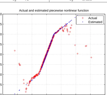
4.3 Hammerstein model where the nonlinearity has memory . . . 41 4.4 The actual and estimated nonlinear function. RMSE = 0.8402 . . . . 44 4.5 Block diagram of a Wiener model . . . 45 4.6 Block diagram of a Wiener model the case that the nonlinear function is
identity . . . 50 4.7 A non-invertible nonlinear function of various break points and slopes . 51 4.8 The equivalent model when small signal is used . . . 52 4.9 The designed system to obtain all the nonlinear function and breakaway
points . . . 52 4.10 Equivalent modified system . . . 53 4.11 The estimated nonlinear function in the case that there is no noise. RMSE
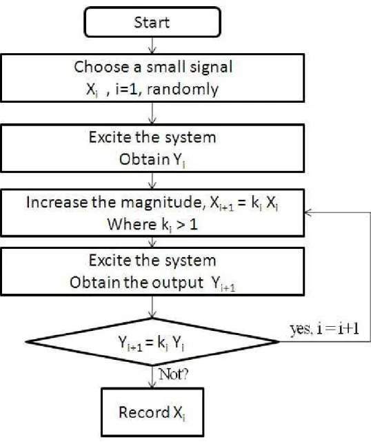
= 0.2822 . . . . 55 4.12 The flowchart for choosing the optimal signal to identify the system. . . . 58 4.13 The actual Wiener model is as at the top figure. We can put the gain in
front of the filter when small signals are used as in the bottom figure. . . 59 4.14 The designed system for identifying the whole of static nonlinear function. 59 4.15 The actual and estimated static nonlinear function. . . 61 4.16 The static nonlinear function sinc(u)u2, and the margins where it can be
approximated by some linear gains. . . 62 4.17 Signals on various points of the Wiener system. Upper plot: input to the
system, middle plot : output of the linearity which is also input to the nonlinearity, bottom plot: output of the whole system. . . 64 4.18 The histogram of the input and output data. As it is seen both seem to
have gaussian distribution of different mean and standard deviation . . . 65 4.19 Non-invertible sin(x)x is modeled with an accurate precision. RMSE =
0.1682 . . . . 66 4.20 The designed closed loop Wiener system for control. . . 67 4.21 A controller is added to make the overall system stable and meet design
4.22 The step response of the closed loop system is unstable. . . 68
4.23 After the controller is added the system became stable. . . 69
4.24 Actual nonlinearities and their inverses. . . 70
4.25 Sinusoidal response of the actual filter. . . 70
4.26 Sinusoidal response of the filter. The response is oscillatory for the chosen integral controller gain. . . 71
4.27 Sinusoidal response of the filter. The controller gain is still not appropriate 71 4.28 Sinusoidal response of the filter. The oscillations have died. . . 72
5.1 The Wiener-Hammerstein system . . . 74
5.2 The Wiener-Hammerstein system as a Hammerstein model . . . 76
5.3 The equivalent Wiener-Hammerstein system when small signals are used. 77 5.4 The equivalent Wiener-Hammerstein system when small signals are used. E(z) is convolution of the first and second filter. . . 79
5.5 The poles and zeroes of actual and estimated filter. . . 81
5.6 Step responses of actual and estimated filters at various points. As it is seen in the bottom figure both responses are almost indistinguishable . . 81
5.7 The actual and estimated output, top plot: correct sharing, bottom: wrong sharing. . . 82
5.8 The designed system to model the static nonlinearity so that the identifi-cation be complete. . . 83
5.9 The outputs of both estimated filters are plotted against each other. The first one is the true nonlinearity, the last one is the true estimated nonlin-earity. . . 84
List of Tables
3.1 Actual and estimated linear parameters . . . 21
3.2 Actual and estimated linear parameters . . . 30
3.3 Correlation and RMSE errors by LS-SVR . . . 31
3.4 Correlation and RMSE errors by LS-SVR mK . . . 31
3.5 Correlation and RMSE errors by Neural Networks . . . 31
4.1 Actual and identified AR parameters . . . 40
4.2 Actual and Estimated MA parameters . . . 40
4.3 Actual and identified AR parameters . . . 43
4.4 Actual and Estimated MA parameters . . . 44
4.5 Actual and identified AR parameters . . . 48
4.6 Actual and Estimated MA parameters . . . 48
4.7 Ar parameters of actual and estimated Wiener Model . . . 54
4.8 MA parameters of actual and estimated Wiener Model . . . 55
4.9 AR parameters of actual and estimated Wiener Model . . . 60
4.10 MA parameters of actual and estimated Wiener Model . . . 60
4.11 AR parameters of actual and estimated Wiener Model . . . 66
4.12 MA parameters of actual and estimated Wiener Model . . . 67
5.1 AR parameters of actual and estimated Wiener Model . . . 80
5.2 MA parameters of actual and estimated Wiener Model . . . 80
5.3 Goodness-of-fit (gof) and normalized mean absolute error (nmae) of the proposed model SVR model , LSL model and Hill Huxley model . . . 86
Chapter 1
INTRODUCTION
System identification in its broadest sense is a powerful technique for building accurate mathematical models of complex systems from noisy data [1]. In this thesis, we mainly deal with Bilinear, Wiener and Hammerstein type nonlinear systems, and their various combinations. These type of systems have simple structures, which is composed of a cas-cade combination of a static nonlinear block with a linear block, see Figures 1.1, 1.2. In many cases, we will model the linear system as a filter, and use the term linear system and filter interchangeably. Although these structures are quite simple, these models are used quite frequently in many control applications, and many identification methods have been developed for these structures, see e.g [2], [3], . We first note that, various combinations of these models, e.g. Wiener-Hammerstein, or Hammerstein-Wiener, can also be considered as a new model. Also, identification of Hammerstein and Hammerstein-Wiener models are easier as compared to the identification of Wiener and Wiener-Hammerstein models. We will mainly focus on identification of the latter systems, e.g. Wiener and Wiener-Hammerstein systems, by improving and/or modifying the identification methods for the Hammerstein and Hammerstein-Wiener systems.
A Hammerstein system may be used for the modeling of many physical systems, see e.g [4]. In [5] it was shown that a power amplifier may be modeled by a Hammerstein system with an IIR filter or by a Wiener system, which will be explained below, with FIR filter. It was also shown in [5] that for high (gain) power amplifiers, Hammerstein models
give better results. In [2], in order to precompensate a power amplifier, a predistorter modeled as a Hammerstein system was developed, and this development was based on an indirect learning architecture (ILA) presented in [2] . In this methodology, instead of ILA, a direct Learning architecture (DLA) can also be used to obtain the required predistorter in Hammerstein form [2].
Figure 1.1: Block diagram of a Hammerstein model
A Wiener model is composed of a linear time invariant system and a static nonlinearity. The linear time invariant system is followed by the static nonlinear function. The block diagram of the model is shown in the Figure 1.2.
Figure 1.2: Block diagram of a Wiener model
Despite its simplicity the Wiener model has been successfully used to describe a number of systems, the most important ones being :
Joint mixing and chemical reaction processes in the chemical process industry. Var-ious types of pH-control processes constitute typical examples, see e.g. [6].
Biological processes, including e.g. vision, see e.g. [4].
Also, as indicated above, a power amplifier may be modeled by using a Wiener system with a FIR filter, see e.g. [5]
What is less well known is that the Wiener model is also useful for the description of a number of situations where the measurement of the output of a linear system is highly nonlinear and non-invertible. Important examples include
Saturation in the output measurements, see e.g. [7]. Dead zones in the output measurements, see e.g. [7].
Output measurements which insensitive to sign, e.g. pulse counting angular rate sensors, see e.g [3].
Quantization in the output measurements. This case has received a considerable interest recently with the emerging techniques for network control systems, see e.g. [8] .
Blind adaptation. This follows since the blind adaptation problem can sometimes be cast into the form of a Wiener system, see e.g. [9]
Wiener models have also been successfully used for extremum control. A main moti-vation for the use of Wiener models is that the dynamics is linear, a fact that simplifies the handling of properties like statistical stationarity and stability, as compared to when a general nonlinear model is applied.
We will also deal with NARX (Nonlinear Auto-Regressive with eXogenous inputs) systems. These type of systems are also applied successfully to model many physical, biological and other phenomenons. For example, in mechanical models for vibration analysis specific polynomial nonlinearities are often used to describe well-known nonlinear elastic or viscous behaviours, see e.g [10]. The well-known Bilinear systems can also be considered as a subset of NARX models. Many objects in engineering, economics, ecology and biology etc. can be described by using a bilinear system, see e.g [11]. The bilinear systems are the simplest nonlinear systems which are similar to a linear system in its form, [12]. In literature, mainly least-squares (LS) techniques and/or black box modeling are used for the identification of NARX, and in particular bilinear systems.
In this thesis we use Least Squares-Support Vector Machines (LS-SVM) to identify the systems introduced above. The aim of identification is to determine both the linear part and the nonlinearity in the system. The linear part represents a Linear Time Invariant, Single Input, Single Output (SISO) discrete time systems, hence can be modeled by a transfer function H(q−1), where q−1 denotes unit delay operator. H(q−1) can be given
as a ratio of two polynomials, namely the numerator and denominator polynomials, and the knowledge of the orders of these polynomials are also required in many cases. In the identification of Wiener systems the invertibility of the nonlinearity is required in various works available in the literature, see e.g. [13], [14] and [15]. Recently, LS-SVM are applied to the identification of Hammerstein systems, see [16]. However, since each system has its own structure, we cannot apply the approach proposed in [16] to Wiener or Wiener-Hammerstein systems, since the optimization problem to be solved becomes highly nonlinear and consequently to obtain an optimal solution becomes very difficult.
In [1] it is proposed that the same method applied to identify Hammerstein systems can be applied to identify Wiener systems too, by changing the role of input and output given that the nonlinearity is invertible. In this thesis we tested this conjecture through various simulations, and our results indicates that this conjecture does not hold in general.
Our contributions in this thesis can be summarized as follows:
For the identification of NARX type systems by using SVM, we have developed a new formulation which improves the identification performance significantly , compared to usual SVM, LS-SVM and PL-LSSVM (Partial Linear- Least Squares Support Vector Machines).
By using LS-SVR (Support Vector Regression ) we have developed a new formula-tion to determine the order of the filters.
Many identification algorithm for Hammerstein systems require that nonlinear block be static, i.e memoryless. We relaxed this assumption and proposed a method for the identification of Hammerstein systems whose nonlinear block has a finite memory. Note that in this case, the usual static nonlinear block of Hammerstein
model is replaced by a non-static nonlinear block.
We have developed new formulations for the identification of Wiener systems, which does not require the nonlinear block to be invertible. Note that many identification schemes proposed in the literature for Wiener systems assume that the nonlinear block be invertible.
We designed feedback control schemes for the control of Wiener systems by using SVM.
In [16] Hammerstein systems are identified by using LS-SVM, and the identification of Wiener-Hammerstein systems by using LS-SVM is set as a future problem. We developed a methodology for the identification of Wiener-Hammerstein systems by using LS-SVM.
In Chapter 2, we first give a brief description about system identification and some procedures. Then we provide some mathematical preliminaries that are necessary for the development of the work which will be presented in this thesis. Chapter 3 addresses the mathematical model and the algorithm we developed for identification of NARX systems. We first obtain the performance of the usual LS-SVM, then we compare it with the performance of Neural Networks. Then we comment on the improvement we obtained on the performance in the identification of NARX systems. In Chapter 4, we show how LS-SVM are used for identification of Hammerstein systems. Then we modify, and design that approach in various ways to identify Wiener systems and to control them. We also compare and contrast our proposed algorithm with the existing algorithms presented in [17] and [18] in terms of the mean squared errors between outputs. In Chapter 5 we propose a novel methodology for the identification of Wiener-Hammerstein systems. by using LS-SVM and compare the performance with some other existing methodologies, see e.g. [19]. Finally we give some concluding remarks in Chapter 6.
Chapter 2
SYSTEM IDENTIFICATION AND
PRELIMINARIES
In this chapter, basic concepts of system identification are explained and some mathe-matical preliminaries are given briefly. We will introduce system identification procedure. Then the main systems we deal with in this thesis, namely Wiener and Hammerstein sys-tems will be introduced. Their application areas will be explained briefly. Then we will present some basic formulations for Support Vector Machine (SVM) classification and regression.
2.1
System Identification
System identification is a general term that is used to describe mathematical tools and algorithms that build dynamical models from measured data. A dynamical system is considered to be as in Figure 2.1 The input signal is ut and the system may have some
disturbances vt. We are able to determine the input signal but not the disturbances.
Sometimes the input signal may also be assumed to be unknown. The output is assumed to be obtained with some measurement errors as usual.
The need for a model to represent a physical system has various reasons. Consider a human body muscle system. After Spinal Cord Injury (SCI), the loss of volitional
Figure 2.1: A dynamic system with input ut output yt and disturbance vt
muscle activity triggers a range of deleterious adaptations. Muscle cross-sectional area declines by as much as 45 % in the first six weeks after injury, with further additional atrophy occurring for at least six months, see e.g. [19]. Muscle atrophy impairs weight distribution over bony prominences, predisposing individuals with SCI to pressure ulcers, a potentially life threatening secondary complication. The neuron (nerve cell) is the fundamental unit of the nervous system. The basic purpose of a neuron is to receive incoming information and, based upon that information, send a signal to other neurons, muscles, or glands. Neurons are designed to rapidly send signals across physiologically long distances. They do this using electrical signals called nerve impulses or action potentials . When a nerve impulse reaches the end of a neuron, it triggers the release of a chemical, or neurotransmitter, see e.g. [20]. The input signal for a muscle is also those signals from neuron cells. The output in such a system is the torque applied by the muscle. Now considering all these relations , the system that transfer the signals from neuron cells to a torque applied by the muscle is a highly complex system. It is composed of a series of biological, chemical, electrical and mechanical processes, and it may be impossible to find an exact mathematical representation of all these processes. Instead we model all these processes by a mathematical structure (in this thesis by a Wiener-Hammerstein model) and try to find the model parameters such that the input (e.g neuron cells signals) and output (e.g torque applied by muscle) relations are satisfied. In Figure 2.2 the pictures of muscles are shown.
In many cases the primary aim of modeling is to aid the controller design process. In other cases the knowledge of a model can itself be the purpose, as for example when describing the effect of a drug. If the model justifies the measured data satisfactorily
Figure 2.2: Torque applied to ankles which is stimulated by neuron cells’ inputs then it may also be used to justify and understand the observed phenomena. In a more general sense modeling is used in many branches of science as an aid to describe and understand reality [21].
2.1.1
Types of Models
A system can be modeled as a box with an input and output. Then the problem is how to model the box. In literature, more emphasis is given on mainly three types of modeling, namely white, gray and black box modeling . White box models are the results of diligent and extensive physical modeling from first principles. This approach consists of writing down all known relationships between relevant variables and using software support to organize them suitably. For a gray box model we may not know the physical model exactly. Nevertheless, we can construct a mathematical model to describe it and try to find the parameters of the model based on measured data. For a black box model no prior model is available, see e.g. [22].
Systems can be either symbolic such as digital computers or numeric. Numeric sys-tems can also be classified as static, dynamic, linear, nonlinear etc. A model can be characterized by three components: first, its structure; secondly the parameters related to this structure; and finally the input signals which are used to excite the system. A structure is a mathematical form and is instantiated by its parameters. The input signals should be chosen carefully for best estimation of the parameters.
2.1.2
Typical System Identification Procedure
In general terms, an identification experiment is performed by exciting the system (using some sort of input signal such as a step, a sinusoid or a random signal -etc.) and observing its input and output over a time interval. These signals are normally recorded in a computer mass storage for subsequent ’information processing’. We then try to fit a parametric model of the process to the recorded input and output sequences. The first step is to determine an appropriate form of the model ( typically a linear difference equation of a certain order). As a second step, some statistically based methods are used to estimate the unknown parameters of the model (such as the coefficients in the difference equation). In practice, the estimation of the structure and the parameters are often done iteratively. This means that a tentative structure is chosen and the corresponding parameters are estimated. The model obtained is then tested to determine whether it is an appropriate representation of the system. If this is not the case, some more complex model structures may be considered, its parameters should be estimated, the new model should be validated, etc. The overall identification process may be given by a flowchart as shown in Figure 2.3, which summarizes the basic steps involved in the process, see e.g. [21].
2.2
Support Vector Machines For Various Tasks
Support vector machines (SVM) are basically used for pattern recognition and in partic-ular for classification tasks. For simplicity, let us assume that the patterns belong to the distinct classes, say C1 and C2. Furthermore let us assign class membership value as +1 if a pattern belongs to C1 and −1 if a pattern belongs to C2. More precisely, let us assume that the patterns are represented by L dimensional vectors, i.e xi ∈ RL for pattern xi,
and let us associate an output value yi for xi such that if xi ∈ C1, we have yi = +1,
and if xi ∈ C2 we have yi = −1. Furthermore let us assume that we have N training
samples, each are represented by a pair {xi, yi}, i = 1, . . . , N . For pattern recognition
L dimensional patterns xi and class labels yi
{x1, y1}, . . . , {xN, yN} ∈ RL× {±1}, (2.1)
such that f will correctly classify new examples (x, y). That is, f (x) = y for examples (x, y) which are generated from the same underlying probability distribution P (x, y) as the training data. If we put no restriction on the class of functions that we choose our estimate f from, even a function that does well on the training data for example by satisfying f (xi) = yi need not generalize well to unseen examples. Suppose that we do
not have additional information on f (for example, about its smoothness). Then the values on the training patterns carry no information whatsoever about values on novel patterns. Hence learning is impossible, and minimizing the training error does not imply a small expected test error. Statistical learning theory, or VC (Vapnik-Chervonenkis) theory, shows that it is crucial to restrict the class of functions that the learning machine can implement to one with a capacity that is suitable for the amount of available training data. For more information, please refer to [23].
Hyperplane classifiers
Given the training set, {xi, yi}, i = 1, . . . , N , and a parameterized form of the
func-tion f (.) : RL → {±1}, finding the parameters of f (.) is of crucial importance for the
classification problem as stated above. There are various ways for the solution of this problem, see e.g. [24]. and utilizing learning algorithms which basically give us an up-date rule/algorithm to find these coefficients, is a frequently used method. To design learning algorithms, we thus must come up with a class of functions whose capacity can be computed. SV classifiers are based on the class of hyperplanes as given below:
< w, ϕ(x) > +d = 0 w ∈ RL, d ∈ R, (2.2)
where w ∈ RL and d ∈ R are unknown parameters to be found, < ., . > represents the
standard inner product in RL, x
i ∈ RL is the pattern vector and ϕ(.) : RL → RH is
given as:
f (x) = sign(< w, ϕ(x) > +d), (2.3) where sign(.) is the standard signum function, i.e
sign(t) = +1, if t ≥ 0, −1, if t < 0 (2.4)
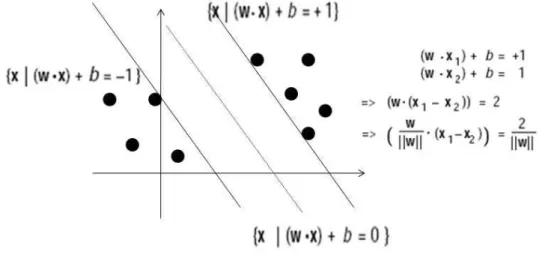
We note that the hyperplane given by ( 2.2) separates the pattern space into two half spaces, if this hyperplane separates C1 and C2, then the signum function achieves correct classification. One can show that the optimal hyperplane, defined as the one with the maximal margin of separation between the two classes (see Figure 2.4), has the lowest capacity [23]. It can be uniquely constructed by solving a constrained quadratic
opti-Figure 2.4: Optimal hyperplane is the plane that divides convex hulls of both classes. mization problem whose solution w has an expansion w =PNi=1αixi in terms of a subset
of training patterns that lie on the margin (see Figure 2.4). These training patterns, called support vectors, carry all relevant information about the classification problem.
Because we are using kernels, we will thus obtain a nonlinear decision function of the following form, see e.g. [25].
f (x) = sign(
N
X
i=1
Here xi’s represent the support vectors, and K(., .) : RH × RH → R is an appropriate
kernel function. In literature, various kernel functions such as Gaussian, Polynomial, etc. are successfully used [26]. In our work we will mainly utilize Gaussian kernel functions, which are given as K(xi, xj) = e(−kxi−xjk
2)
The parameters αiare computed as the solution
of a quadratic programming problem.
The most important restriction up to now has been that we consider only the classifi-cation problem. However, a generalization to regression estimation,that is, to y ∈ R, can also be given, see e.g. [27]. In this case, the algorithm tries to construct a linear function in the feature space such that the training points lie within a distance ² > 0. Similar to the pattern-recognition case, we can write this as a quadratic programming problem in terms of kernels. The nonlinear regression estimate takes the form
f (x) =
N
X
i=1
αiK(x, xi) + d (2.6)
To apply the algorithm, we either specify ² a priori, or we specify an upper bound on the fraction of training points allowed to lie outside of a distance ² from the regres-sion estimate (asymptotically, the number of SVs) and the corresponding ² is computed automatically. For more information refer to [26].
Chapter 3
A NEW FORMULATION FOR
SUPPORT VECTOR
REGRESSION AND ITS USAGE
FOR BILINEAR SYSTEM
IDENTIFICATION
In this chapter, basic concepts of Support Vector Regression (SVR) are explained. First we will show how nonlinear functions are modeled with SVM in general. We will then show LS-SVM regression in particular and examine its performance. Then we will present performance of Neural Network regression. We will also present a novel methodology and will illustrate its performance compared to usual SVM regression approach and Neural Network approach. We will make comparisons between these three methods in terms of their performances. Finally we will present a novel methodology to determine the order of the filter representing the linear blocks in our model, see Figure 1.1 and 1.2
3.1
Nonlinear System Regression
Any nonlinear function (system) can be modeled with Support Vector Regression (SVR). Support Vector Regression uses the same principle as the Support Vector Machine clas-sification, with only a few minor differences. In the case of classification only two output values are possible. But since we are trying to model a nonlinear function, the output has infinitely many possible values, that is while in classification we have y ∈ {∓1}, here we have y ∈ R. However, the main idea is similar: to minimize the error and maximize the margin between the optimal hyperplanes.
The nonlinear dynamical systems with an input u and an output y can be described in discrete time by the NARX (nonlinear autoregressive with exogenous input) input output model:
y(k) = f (x(k)), (3.1)
where f (.) is a nonlinear function, y(k) ∈ R denotes the output at the time instant
k and x(k) is the regressor vector, consisting of a finite number of past inputs and
outputs. If we assume that the current output y(k) depends on past outputs y(i) for i ∈ [k − ny− 1, k − 1] and inputs u(i) for i ∈ [k − nu− 1, k], where ny and nuare appropriate
integers, then an appropriate regression vector x(k) to be used in 3.1 can be given as follows: x(k) = y(k − 1) ... y(k − ny) u(k) ... u(k − nu) (3.2)
where nu is the dynamical order for the inputs and ny is the dynamical order for the
outputs, i.e. the present output depends on past ny outputs and nu inputs, as explained
above. Hence, with the above notation, we have x ∈ Rnu+ny+1, y ∈ R and f : Rnu+ny+1 →
R. We note that, here the regression relation is deterministic. In a realistic situation, output measurements are usually corrupted by some noise. For such cases, instead of
3.1, we may consider the following regression relation.
y(k) = f (x(k)) + ξ(k), (3.3)
where the regression vector x(.), the output y(.) and the nonlinear function f (.) are the same as explained above; here ξ(.) represents the meausurement noise, and typically modeled by a gaussian noise with zero mean and finite variance. Note that, for notational simplicity we will use the notation ξi to denote ξ(i) in the sequel.
The task of system identification here is essentially to find suitable mappings, which can approximate the mappings implied in the nonlinear dynamical system of (3.1). The function f (.) can be approximated by some general function approximators such as neural networks, neuro-fuzzy systems, splines, interpolated look-up tables, etc. [25]. The aim of system identification is only to obtain an accurate predictor for y. In this work we will show how we may increase the performance of the predictor by using appropriate kernel mappings for each nonlinearity in the function f (.). The details will be given in the sequel.
3.2
LS-SVM Regression
Consider a given training set of N data points {xi, yi} for i = 1, . . . , N , where xi ∈ Rn,
y ∈ R, (note that with the notation of (3.3), we have n = nu+ny+1). Let us assume that
the input output relation is as given by (3.1). Our aim will be based on the training data, to find an estimation of the nonlinear function f (.). Although several techniques may be utilized to estimate f (.), we will use SVM technique introduced in section 2. Hence, referring to (2.6), we will try to approximate the nonlinear function f (.) as follows:
y(x) =< w, ϕ(x) > +d = wTϕ(x) + d, (3.4) where ϕ : Rn→ Rnf, where n
f is left undetermined yet and usually nf ≥ n, d ∈ R. ϕ(.)
is called the feature map; its role is to map the data into a higher dimensional feature space, which could also be infinite dimensional (i.e nf = ∞) in theory. Various forms of
If we use the well-known Least Squares (LS) technique for function approximation by using SVM’s, the approximation problem can be formulated as an optimization problem, which is labeled as LS-SVM. In this case, the standard optimization problem can be given as follows. min w,ξ F (w, ξt) = 1/2kwk 2+ γ/2Xξ2 t (3.5) subject to yt= wTϕ(xt) + d + ξt, ∀t = 1, . . . , N
Note that here k.k is the standard euclidian norm in Rn, i.e kwk2 = wTw. γ is the
penalty term, the bigger it is the less it will be tolerant to error.
Here the quadratic programming problem has equality constraints. The problem is convex and can be solved by using Lagrangian multipliers, αi, see [26]. If there were no
constraints while minimizing the objective function in (3.5) we could have just taken the partial derivative of the objective function and set it to zero. Since the objective function is convex, the point where the derivative is zero would be the solution for the minimiza-tion. But since we have some constraints we have to construct the Lagrangian and set its partial derivatives w.r.t all of its variables and set them to zero. The Lagrangian is given as follows: L (w, d, ξt, α) = F (w, ξt) − N X t=1 αt(wTϕ(xt) + d + ξt− yt). (3.6)
Using the Karush-Kuhn-Tucker (KKT) conditions we obtain the following equations.
∂L ∂w = 0 → w = N X t=1 αtϕ(xt) (3.7a) ∂L ∂d = 0 → N X t=1 αt= 0 (3.7b) ∂L ∂ξt = 0 → αt= γξt, t = 1, . . . , N (3.7c) ∂L ∂αt = 0 → yt= wTϕ(xt) + d + ξt, t = 1, . . . , N (3.7d)
If we put (??) and (3.7c) in (3.7d) we obtain the following: yk= N X t=1 αtϕ(xt)Tϕ(xk) + d + ξk, k = 1, . . . , N (3.8)
Note that in (3.8), we have N equations. We can rewrite (3.8) and (3.7b) as a set of linear equations in the following form:
0 1TN 1N K + γ−1I1TN d α = 0 Y (3.9)
Where K is a positive definite matrix and K(i, j) = ϕ(xi)Tϕ(xj) = e
(−kxi−xj k2)
2σ2 , where
σ is a scaling factor, α = [α1α2. . . αN], 1TNis a vector, whose entries are 1 and d is the bias term. The mapping ϕ(.) can be polynomial, linear etc. In 3.9 a least squares solution is obtained in order to find α and d parameters. Since this is almost standard, we omit the details here, interested reader may refer to [26] for details. After obtaining these parameters, the resulting expression for estimated function will be as the following: Note that 3.9 is a linear equation of the form Az = b, where z = [d α]T is the unknown vector which gives the sum parameters. A LS solution to this equation can be obtained by using various techniques see e.g.[29]. After obtaining the SVM parameters, the regressor function f (.) can be approximated by using (3.4) as,
f (x) = wTϕ(x) + d, (3.10)
If we use (3.7a) in (3.10) we obtain
f (x) =
N
X
k=1
αkϕ(x(k))Tϕ(x) + d. (3.11)
Finally if we denote the kernel K(x, xk) as K(x, xk) = ϕ(x(k))Tϕ(x), we obtain:
f (x) =
N
X
k=1
αkK(x, xk) + d. (3.12)
In order to see the performance of the resulting estimated function we have done various simulations for different systems . Assume that the system dynamics is given by (3.1), where the nonlinear function f (x(k)) is given as:
f (x(k)) = (a0+ a1sin(u(k − 1)) + a2cos(u(k − 2)))y(k − 1)
+(b0+ b1sin(u(k − 1)) + b2u(k − 2))y(k − 2) + c1u(k − 1) + c2u(k − 2) (3.13)
The function f (.) given by 3.13 can be rewritten as
f (xk) = a0yk−1+ f1(uk−1, yk−1) + f2(uk−2, yk−1)
+f3(uk−1, yk−2) + f4(uk−2, yk−2). (3.14a)
f1(uk−1, yk−1) = a1sin(u(k − 1))y(k − 1) (3.14b)
f2(uk−2, yk−1) = a2cos(u(k − 2))y(k − 1) (3.14c)
f3(uk−1, yk−2) = b1sin(u(k − 1))y(k − 2) (3.14d)
f4(uk−2, yk−2) = b2u(k − 2)y(k − 2) (3.14e)
Therefore we can think of f (.) as a function that depends on xk= [uk−1 uk−2 yk−1 yk−2]T.
Hence, this function can be modeled with SVR by using xk as the regressor vector. The
leading formulations will be as the following:
min wx,ek F (w, ξk) = 1/2wTw + γ/2 N X k=r ξk2
subject to y(k) = a0y(k − 1) + b0y(k − 2) + c1u(k − 1) + c2u(k − 2) + wTϕ(x(k)) + d + ξ k, k = r, . . . , N (3.15a) N X k=1 wTϕ(x(k)) = 0 . (3.15b)
The problem is quadratic and the appropriate Lagrangian is:
L (w, ai, bi, ci, d, ξk, α, β) = F (w, ξk) − N
X
k=r
αk(a0y(k − 1) + b0y(k − 2) + c1u(k − 1)
+c2u(k − 2) + wTϕ(x(k)) + ek− yk) − β N
X
k=1
wTϕ(x(k)) (3.16)
∂L ∂w = 0 → w = N X k=r αkϕ(xk) + β N X k=1 ϕ(xk), (3.17a) ∂L ∂a0, b0, c1, c2 = 0 → N X k=r αky(k − i) = 0, i = 1, 2. N X k=r αku(k − i) = 0 i = 1, 2 (3.17b) ∂L ∂d = 0 → N X k=r αk= 0 (3.17c) ∂L ∂ξk = 0 → αk= γξk, k = r, . . . , N (3.17d) ∂L ∂αk
= 0 → yk = a0y(k − 1) + b0y(k − 2) + c1u(k − 1) + c2u(k − 2)
+ wTϕ(x) + d + ξk, k = r, . . . , N (3.17e) ∂L ∂β = 0 → N X k=1 wTϕ(x(k)) = 0 (3.17f)
If we put (3.17a) and (3.17d) into (3.17e) we obtain the following set of linear equations. 0 0 0 1T 0 0 0 0 Yp 0 0 0 0 Up 0 1 Y T p UpT K + γ−1I K0 0 0 0 K0T 1T NΩ1NIm+1 d a c α β = 0 0 0 Yf 0 (3.18)
where a = [a0 b0] and c = [c1 c2]. A LS solution is taken in order to obtain a, c and SVM parameters.
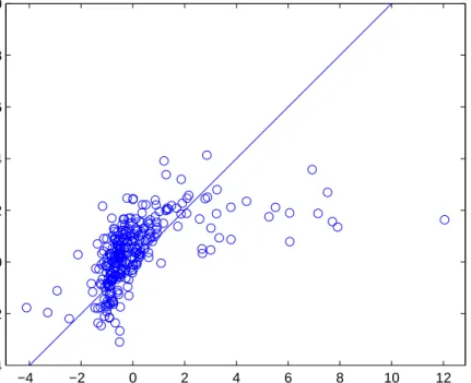
Now let us consider the example given by (3.13) with the actual parameters chosen as a0 = 0.3, b0 = 0.2, c1 = 0.5, c2 = 0.6. with these parameters we simulated the system given by (3.1) , (3.2), (3.13) by using input as a random signal of Gaussian distribution with 0 mean and standard deviation 2. We created N = 300 samples of training data. Noise also has a Gaussian distribution of 0 mean and standard deviation less than 0.2. Then by solving (3.18), we obtained the estimated parameters as shown
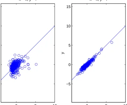
in Table 3.1. By using the same input which is used obtaining the training data, and by using (3.13) with the estimated parameters, we also obtained the estimated outputs. The distribution of actual outputs and estimated outputs are also shown in Figure 3.1. As can be seen from the Figure 3.1 and the Table 3.1, the performance of the scheme as outlined above is not satisfactory.
We will now show the resulting estimated outputs ˆyk and actual outputs in terms
of RMSE (Root Mean Squared Error), output correlation etc. and compare them with neural network regression. And then we will show how we improved these performances by using some new formulations.
−4 −2 0 2 4 6 8 10 12 −4 −2 0 2 4 6 8 10 x y x = x, y = r
Figure 3.1: The actual output values vs the estimated output values.
Table 3.1: Actual and estimated linear parameters Actual parameters Identified parameters
a0 = 0.3 ˆa0 = 0.413
b0 = 0.2 ˆb0 = 0.126
c1 = 0.5 ˆc1 = 0.671
c2 = 0.6 ˆc2 = 0.704
and may be not for some others. We will now compare these results with neural network regression. But with neural networks we will not be able to estimate the parameters of the linear part in (3.14). Only the inputs and outputs will be mapped and both will be compared in terms of some performance criterions such as RMSE, correlation coefficients etc. Regression (R) Values measure the correlation between estimated outputs and targets (actual outputs). While an R = 1 means a close relationship, R = 0 means a random relationship. Mean Squared Error is the average squared difference between outputs and targets (actual outputs). Obviously lower values of RMSE indicates better performance.
3.3
Feedforward Neural Network Regression
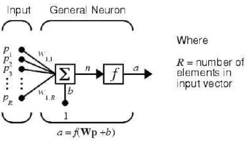
An elementary neuron with R inputs is shown in Figure 3.2. Here P1, . . . , PR denotes
the input values and w1,1, . . . , w1,R denotes their corresponding weights and b represents the bias term. Hence, the weighted sum n can be represented as:
n =
R
X
i=1
w1,iPi+ b (3.19a)
The function f (.) determines the output a , as
a = f (n) (3.19b)
Note that although any function f(.) can be used for neural representations, sigmoidal functions, which will be introduced later , are most frequently used. Moreover, to solve optimization problems, mostly differentiable functions are used.
We can simplify (3.19a) and (3.19b) by introducing the input and weight values as follows.
Multilayer networks often use the log-sigmoid transfer function logsig, which is defined as
logsig(n) = 1
1 + e−λn (3.20)
A typical figure of such a function is given in Figure 3.3. Here λ > 0 is a parameter which determines the steepness of the function around x = 0. Note that as λ → ∞,
Figure 3.2: The neuron model used in the feedforward network.©MATLAB
Figure 3.3: A possible transfer function used to activate neurons.©MATLAB
3.3.1
Feedforward Network
A single-layer network of S logsig neurons having R inputs is shown below in full detail on the left and with a layer diagram on the right.
Mathematical formulation of input output relation of the structure shown in Figure 3.4 is straightforward if we use the representation of single neuron. We can define the weight matrix w as: w = (w1. . . wS)T where wi = (wi,1, . . . , wi,R) i = 1, . . . , S.
More-over, we can define the linear sum vector n, bias vector b, and output vector a similarly as:
Figure 3.4: A Feedforward neural network.©MATLAB
n = (n1. . . nS) b = (b1. . . bS) a = (a1. . . aS). Hence, with this notation, we have
n = WP + b (3.21)
and finally
a = F (.) = F (WP + b) (3.22)
where F (.) : RS → RS is defined as
F (n) = (logsig(n1), . . . , logsig(ns))T, (3.23)
where the superscript T denotes the transpose.
If we concatenate such layers in cascade form, we obtain the so-called multilayer neural networks. It is well known that a 2-layer neural network with linear activation functions in the second layer (e.g f (n) = n in Fig. 3.2) can approximate any continuous function with arbitrary degree of precision, see eg. [30]. For a given function, or for a given training set, the appropriate weights of the neural network can be found by using the so-called Back Propagation Algorithm, see e.g [31]. In this work we will use the MATLAB toolbox for neural network simulations.
The network will be trained with Levenberg-Marquardt backpropagation algorithm (a MATLAB function : trainlm).
Figure 3.5: The actual output values vs the estimated output values using Neural Net-works.
The nonlinear system that is to be modeled is the one that we have used in the previous section, i.e. the function (3.13). The length of the training data is N = 300, the input used to excite the system is the same as before, i.e u(k) = N (0, 2), hence the output is also the same in order for the comparisons be sensible. The performance results are shown in the Figure 3.5. In the Figure 3.5 the target, i.e axis x, denote the actual output, i.e y(k), while axis y denote the estimated output, i.e ˆy(k). The value R denote
the correlation between actual y(k) (target) and estimated outputs ˆy(k) (axis y).
The results show that the Neural Networks perform much better than LS-SVM Re-gression, in terms of both RMSE and correlation (R) values. However, note that here we do not estimate the parameters a0, . . . , c2, but estimate the input-output relation.
3.4
Improved performance using multiple kernels
Now we will show how the overall identification performance can be improved by using multiple kernels. Note that this is similar to the concept of mK kernels used in the literature, see e.g [32]. In the usual SVM regression, the formulation given in Section 3.2 is used. Now we will modify this methodology and interpret the resulting perfor-mance. Now consider the system given previously, i.e. by (3.1) , (3.2) and (3.13). In order to model this system with LS-SVM we used only a regression vector of form
xk = [uk−1 uk−2 yk−1 yk−2]T. In that case the resulting model has only one kernel
function. We can divide the regression vector and construct a kernel from each divided vector. Now consider the nonlinear function given by (3.14a)- (3.14e). Instead of using only a single SVM for the total nonlinear function, we could utilize one SVM for each of the nonlinear parts. More precisely, we could express f1, f2, f3, f4 as:
f1(uk−1, yk−1) = waT1ϕ(xa1(k)) + d1 (3.24a)
f2(uk−2, yk−1) = waT2ϕ(xa2(k)) + d2 (3.24b)
f3(uk−1, yk−2) = wbT1ϕ(xb1(k)) + d3 (3.24c)
f4(uk−2, yk−2) = wbT2ϕ(xb2(k)) + d4 (3.24d)
where xai, xbi i = 1, 2 are given as:
xa1 = u(k) y(k − 1) , xa2 = u(k − 2) y(k − 1) , xb1 = u(k − 1) y(k − 2) , xb2 = u(k − 2) y(k − 2) , (3.25) If we substitute (3.24a)- (3.24d) in (3.14a), we obtain
y(k) = f (x(k)) = (a0y(k − 1) + b0y(k − 2) + c1u(k − 1) + c2u(k − 2) +wT a1ϕ(xa1(k)) + w T a2ϕ(xa2(k)) + w T b1ϕ(xb1(k)) + w T b2ϕ(xb2(k)) + d + ek, k = r, . . . , N (3.26) where d = d1+ d2 + d3+ d4
As seen in the above equation instead of only one SVM , 4 SVM are used to model the function f (.). To obtain the optimal points, the optimization problem is constructed as follows: min wx,ξk F (w, ξk) = 1/2 X x wT xwx+ γ/2 N X k=r ξ2 k
subject to y(k) = f (x(k)) = (a0y(k − 1) + b0y(k − 2) + c1u(k − 1) + c2u(k − 2) +waT1ϕ(xa1(k)) + w T a2ϕ(xa2(k)) + w T b1ϕ(xb1(k)) + w T b2ϕ(xb2(k)) + d + ξk, k = r, . . . , N (3.27a) N X k=1 wxTϕ(xx(k)) = 0 for x = a1, a2, b1, b2. (3.27b)
The problem is quadratic and the associated lagrangian can be given as:
L (w, a, b, c, d, ξk, α, β) = F (w, ξk) − N
X
k=r
αk(a0y(k − 1) + b0y(k − 2) + c1u(k − 1)+
c2u(k − 2) + waT1ϕ(xa1(k))+w T a2ϕ(xa2(k)) + w T b1ϕ(xb1(k)) + w T b2ϕ(xb2(k)) + d + ξk− yk) − X x=a0,b0,c1,c2 βx N X k=1 wTxϕ(xx(k)) (3.28)
Again by using the Karush-Kuhn-Tucker (KKT) conditions we obtain the following equations. ∂L ∂wx = 0 → wx = N X k=r αkϕ(xk) + βx N X k=1 ϕ(xk), x = a0, b0, c1, c2 (3.29a) ∂L ∂a0, b0, c1, c2 = 0 → N X k=r αky(k − i) = 0, i = 1, 2. N X k=r αku(k − i) = 0 i = 1, 2 (3.29b) ∂L ∂d = 0 → N X k=r αk= 0 (3.29c) ∂L ∂ek = 0 → αk= γξk, k = r, . . . , N (3.29d) ∂L ∂αk = 0 → (3.27a) (3.29e) ∂L ∂βk = 0 → N X k=1 wT xϕ(xx(k)) = 0 for x = a1, a2, b1, b2. (3.29f)
If we put (3.29a) into (3.27a) and (3.29f), the following equations are obtained respec-tively:
y(k) = a0y(k − 1) + b0y(k − 2) + c1u(k − 1) + c2u(k − 2)
+ N X t=r αtKa1(t, k) + βa1 N X t=1 Ka1(t, k) + N X t=r αtKa2(t, k) + βa2 N X t=1 Ka2(t, k) + N X t=r αtKb1(t, k) + βb1 N X t=1 Kb1(t, k) + N X t=r αtKb2(t, k) + βb2 N X t=1 Kb2(t, k) + d + ek , k = r, . . . , N (3.30) N X k=1 N X t=r αtKa1(t, k) + βa1 N X k=1 N X t=1 Ka1(t, k) = 0 (3.31a) N X k=1 N X t=r αtKa2(t, k) + βa2 N X k=1 N X t=1 Ka2(t, k) = 0 (3.31b) N X k=1 N X t=r αtKb1(t, k) + βb1 N X k=1 N X t=1 Kb1(t, k) = 0 (3.31c) N X k=1 N X t=r αtKb2(t, k) + βb2 N X k=1 N X t=1 Kb2(t, k) = 0 (3.31d)
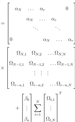
The equations given above can be put into a set of linear equations, whose matrix form is given below:
0 0 0 1T 0 0 0 0 Yp 0 0 0 0 Up 0 1 Y T p UpT K + γ−1I K0 0 0 0 K0T 1T NΩ1NIm+1 d a c α β = 0 0 0 Yf 0 (3.32)
where a = [a0 b0] and c = [c1 c2]. A LS solution is taken in order to obtain a, c and SVM parameters.
Although the linear part parameters are not estimated accurately in both procedures ( 1K and mK) the overall results are accurate in terms of RMSE. Now let us consider
0 5 10 −5 0 5 10 15 x y x = x, y = r 0 5 10 −5 0 5 10 15 x y x = x, y = r
Figure 3.6: The corrleation between actual and estimated output. Left using LS-SVR, right using LS-SVR mK.
the example given by (3.13) again with the actual parameters chosen the same as a0 = 0.3, b0 = 0.2, c1 = 0.5, c2 = 0.6. with these parameters we simulated the system given by (3.1) , (3.2), (3.13) by using input as a random signal of Gaussian distribution with 0 mean and standard deviation 2. We created N = 300 samples of training data. Noise also has a Gaussian distribution of 0 mean and standard deviation less than 0.2. Then by solving (3.32), we obtained the estimated parameters as shown in Table 3.2. By using the same input which is used obtaining the training data, and by using (3.13) with the estimated parameters, we also obtained the estimated outputs. The distribution of actual outputs and estimated outputs are also shown in Figure 3.7. As can be seen from the Figure 3.7, the performance of the scheme as outlined above is satisfactory.
Finally to further signify the effectiveness of using LS-SVR mK some performance comparisons are shown in the Tables 3.3, 3.4 and 3.5. As can be seen from the tables the LS-SVR mK and neural network regression performs much better than the conventional LS-SVR regression. If we compare LS-SVR mK and neural networks , each
Figure 3.7: The actual output values vs the estimated output values using LS-SVR mK. Table 3.2: Actual and estimated linear parameters
Actual parameters Identified parameters
a0 = 0.3 ˆa0 = 0.406
b0 = 0.2 ˆb0 = 0.135
c1 = 0.5 ˆc1 = 0.683
c2 = 0.6 ˆc2 = 0.710
has better performance for some combinations and worse performance for some other combinations of chosen parameters. But the best performance is achieved by LS-SVR mK for the test data.
3.5
Determining the orders of an ARMA(p,q) by
LS-SVR
In this section we will give a novel application of SVR to determine the orders of a linear filter, i.e the degrees of numerator and denominator polynomials. In the following chapters we will mainly assume that we know the orders of the filters in the systems to
Table 3.3: Correlation and RMSE errors by LS-SVR RMSE Correlation method γ σ train test trainreg testreg
LS-SVR 1000 0.5 0.4119 1.4834 0.8922 0.4682 1500 0.3872 0.6744 0.9100 0.9003 2000 0.5650 1.4034 0.8778 0.5772 1000 1.0 0.9421 1.7880 0.8715 0.3967 1500 0.6797 1.1063 0.9119 0.6826 2000 0.3800 0.7726 0.9329 0.8827
Table 3.4: Correlation and RMSE errors by LS-SVR mK RMSE Correlation method γ σ train test trainreg testreg
LS-SVR 1000 0.5 0.0233 0.1313 0.9996 0.9878 1500 0.0111 0.2057 0.9998 0.9953 2000 0.0245 0.1197 1.00008 0.9751 1000 1.0 0.0038 0.1732 1.0000 0.9806 1500 0.0188 0.6185 1.0000 0.9949 2000 0.0011 0.6631 1.0000 0.9955
Table 3.5: Correlation and RMSE errors by Neural Networks RMSE Correlation method ]Neurons ]Layer train test trainreg testreg NN LM BackProp
15 1 0.0056 0.3633 0.9999 0.9954 20 0.0067 0.2715 0.9998 0.9997 25 0.0074 0.3768 0.9999 0.8979
be identified, i.e we assume that we know the number nu and ny in (3.2). There are
various ways to determine the orders of the filter in the literature, [33]. In the sequel we will give a novel way to determine these orders. We will use LS-SVR to determine these orders. Our method is based on a trial and error technique. The order for which the error is least will be taken as the correct order. The AR (i.e ny in 3.2) and MA orders
(i.e nu in 3.2) are determined separately. Consider an arma(p,q) filter given as follows:
yk = p X i=1 aiyk−i+ q X j=0 bjuk−j (3.33)
The aim is to determine the values of p which is AR(Auto-Regressive) order and
q which is MA(Moving-Average) order. By using LS-SVR we can train support vectors
such that the input and output training data {uk, yk}Nk=1 are mapped with the least error.
We can train SVR in various ways. The difference is the order of the training vector xk,
where xk is as defined before
x(k) = y(k − 1) ... y(k − ny) u(k) ... u(k − nu) (3.34)
The filter will be modeled as in (3.35), similar to the mapping in (3.4).
y(xk) =< w, ϕ(xk) > +d = wTϕ(xk) + d, (3.35)
For a training data {uk, yk}, we may construct the following optimization problem.
min
w,ξ F (w, ξk) = 1/2kwk
2+ γ/2Xξ2
k (3.36)
subject to yk = wTϕ(xk) + d + ξk, ∀k = 1, . . . , N
We will mainly change the lags ny and nu and compare the errors between the actual and
estimated outputs. Note that the lag nu can be considered to be related to the order q,
The solution to the optimization problem (3.36) is the same as the solution (3.9) in section 3.2. The resulting estimated outputs can be given as :
ˆ yk = N X t=1 αkK(xt, xk) + d (3.37)
At the first iteration the lag nu is set to 0, i.e only the current input is present in the
regression vector xk, whereas the lag ny is increased by 1 for each training iteration. The
MSE (Mean Squared Error ) between the actual yk and ˆyk is computed. As can be seen
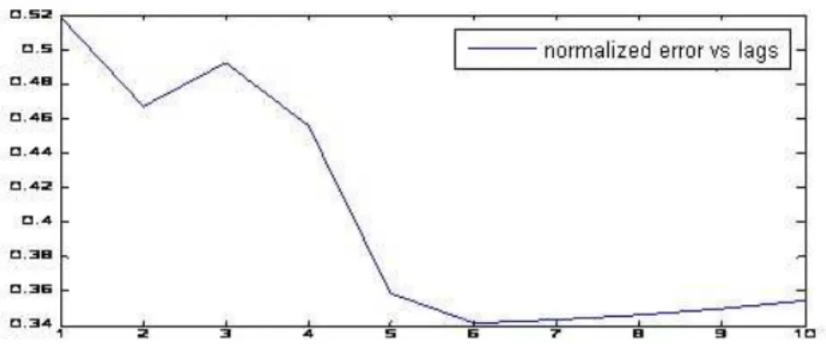
from the Figure 3.8, the error is maximum for the lag ny = 1, then it decreases up to
the lag ny = 6, which is the true order, i.e p = 6, then it increases. To obtain the order
q, i.e numerator order, a similar approach is applied. The lag ny is taken to be 0 at
first iteration, the lag nu is increased starting from nu = 1 at first iteration. The errors
between actual yk and ˆyk are computed, the lag for which the error is minimum is taken
to be true order. This can be seen from the Figure 3.9. The true order is 3 and the error is minimum at that point. So in this way the order of the filter is obtained correctly.
Figure 3.8: The normalized error between actual and estimated outputs as the lags increases.
Various input signals are used to see the best results. Choosing input as a signal of uniform distribution between some points [p1, p2] did not give accurate results. The best results are obtained when the input signal is chosen to be a random variable of normal distribution.
In order to obtain the numerator order i.e.q) more attention is required. The regression vector is composed of only input values. For the previous case the lag for input was chosen
to be 0 , that is only the current input is taken. But in this case, there is no output value in the regression vector. Also the SVM parameters sigma, σ, gamma γ need to be chosen carefully for optimal results.
Figure 3.9: The normalized error between actual and estimated outputs as the lags increases for numerator order.
Chapter 4
IDENTIFICATION AND
CONTROL OF WIENER
SYSTEMS BY LS-SVM
In this chapter we will first show how a method which utilizes LS-SVM for the identifi-cation of Hammerstein systems. We then propose a novel method when the nonlinearity in Hammerstein systems has a finite memory. We will then give some results on Wiener systems when the same procedure used for identification of Hammerstein systems is ap-plied. Then we will develop our own methodology to improve the performance of the identification of Wiener systems. We then propose a novel method for the control of Wiener systems. Finally we will make comparisons between performances of all these procedures.
4.1
Hammerstein Model Identification Using LS-SVM
In this section we will briefly explain how Hammerstein models can be identified by using LS-SVM. In the following sections we will explain how the method proposed in Chapter 2 can be used for the identification of Hammerstein type systems and how it can be modified for the identification of Wiener type systems . The block diagram of a
Hammerstein model is given in the Figure 4.1 for convenience.
Figure 4.1: Block diagram of a Hammerstein model
The input signal ut is used to excite the system and has a normal distribution of 0
mean and standard deviation 2. The reason that such a signal is used will be explained later. The dynamics of the whole structure can be given as follows:
yk = n X i=1 aiyk−i+ m X j=0 bjf (uk−j) + ek. (4.1)
Here k ∈ Z, uk, yk ∈ R, denotes the input and measured outputs. The so-called
equation error ek is assumed to be a white noise and m and n are the order of the
numerator and denominator in the transfer function of the linear model. Also the orders
m and n are assumed to be known a priori, [16]. The aim of identification is to estimate
the parameters ai and bj i = 1, . . . , n, j = 1, . . . , m. The static-nonlinear function
f (.) is also to be estimated. If f (.) is known, the parameters ai, bj in (4.1) could easily
be estimated by using standard optimization techniques, such as LSE. Hence we will use SVM to model the static-nonlinear function f (.). As introduced in chapter 2, the SVM approximation of the nonlinear function f (.) can be given as follows:
f (uk) = wTϕ(uk) + d (4.2)
For the meaning of various parameters in 4.2, see Chapter 2. If we use (4.2) in (4.1), we obtain yk = n X i=1 aiyk−i+ n X j=0 bj(wtϕ(uk) + d) (4.3)