' г к : , · · I »r«. | P · ,.* f f m Г Ч'· ^ -’ ^ 5! ? * *»ί φ . jf ^ . . й « ^· j * >· f · >■? * -«« ц t ¡ tti; Й »« W í ϊ ι/ < i : ‘ · г- i 't' .( ' .· ' < - ■■ · < \ ’ ’"f i· ?! Г-'' i " " '* *' · '.'· «■ .η •' "' ‘• t г .'·· “ ?j T-· г í >’v i ’·^ '’ " ' · • 'Í;^ '· ?'' « î · ·’· , .: ''^í;y i^·' l > ’ '^• Í Î H 'İ £ · ^" ít ‘ . '¡■ ’s i ..V' ' ■ ’ / ¿ ‘ «» ir fi («¿ ^ ^· /t,‘i i. ^Í í' 5i '; 4Í t¿ ¡r^«jt 4 hk 'í í^ '^ /4 :· 4v W -1 ÍL o^ '
A ií
SK
sft
iS
S І
І Ш
І П
Ш
m
I *'* ’ · í''· ,Λ ,* * .Ь Λ ^-^ ,♦y . ^ . ^л . .4· M , ίζ _ ΐ ^ * ”^ Г * ''"" · f ? ?* ^· i*' Ş » f f' « s i s e a « яш йб із ш · ·.·' . .·.' < · V ’ ■ . ., ( , ' λ t sit-' sit-'^ ¿ ¿f 'v, 'C' İ : .j) ' ' ¡*fr - Лии ^íí i^w . <ί ·'W * Ä i s9e
eı
€G
¥·
G 't o ts MJ . ■ f ^. f ? f t * ’.· ■ ■ ' ' ’ , " i Г : : {.; r *.!. r Í f?U 5 «? : ; ' ■' ';. ■ · ■ Í Í. 1 ; " ? C ' If ·^
Ί
j ö 1 Й " i ? p;i
i? fs I İl 3 f oî I İl ЙІ i- i H d I i flШ
ÍI Í 2 i i i s ' Ϊ i « » - ж'Щ
.щ
^
*■·■ h · * K Ы İH ■ T s ε f ' · n: г iâ iA df î, г г o Ш Æ Ú v Ш ! · ■ ; . #■ ! ( !>i ¿ r ”t 'ı.y Й '; H vROBUST ADAPTIVE FILTERING ALGORITHMS
FOR IMPULSIVE NOISE ENVIRONMENTS
A THESIS
SUBMITTED TO THE DEPARTMENT OF ELECTRICAL AND ELECTRONICS ENGINEERING
AND THE INSTITUTE OF ENGINEERING AND SCIENCES OF BILKENT UNIVERSITY
IN PARTIAL FULFILLMENT OF THE REQUIREMENTS FOR THE DEGREE OF
MASTER OF SCIENCE
By
Gül Aydın
July 1996
G-üL· /IVQ/A/
farafintfcui fr«|*|idniniflir·τ κ
'5402.. 3 •АЪЪ
I certify that I have read this thesis and that in my opinion it is fully adequate, in scope and in quality, as a thesis for the degree of Master of Science.
^ ^ _________
Assoc. Prof. Dr. A. Enis ^etin(Supervisor)
I certify that I have read this thesis and that in my opinion it is fully adequate, in scope and in quality, as a thesis for the degree of Master of Science.
Assist. Prof. Dr. Orhan Arikan
I certify that I hcive read this thesis and that in my opinion it is fully adequate, in scope cuid in quality, cis a thesis lor the degree of Mcister of Science.
Assist. Prof. Dr. Billur Bcirshan
Approved for the Institute of Engineering and Sciences:
Prof. Dr. Mehrnel^paray
ABSTRACT
ROBUST ADAPTIVE FILTERING ALGORITHMS
FOR IMPULSIVE NOISE ENVIRONMENTS
Gül Aydın
M.S. in Electriccil and Electronics Engineering
Supervisor: Assoc. Prof. Dr. A. Enis Çetin
•July 1996
In this thesis, robust adaptive filtering algorithms are introduced for im pulsive noise environments which can be modeled as o;-stable distributions and/or c-contarninated Gaussian distributions. The algorithms are devcrloped using the Fractional Lower Order Statistics concept. Robust perf()rrnance is obtained.
Keywords : Adaptive F'iltering, a-stable distributions, Fractional Lower Or der Moments, e-contaminated Gaussian distributions
ÖZET
PATLAMALI GÜRÜLTÜLÜ ORTAMLAR İÇİN DAYANIKLI
SÜZGEÇLEME ALGORİTMALARI
Gül Aydın
Elektrik ve Elektronik Mühendisliği Bölümü Yüksek Lisans
Tez yöneticisi: Assoc. Prof. Dr. A. Enis Çetin
Temmuz 1996
Bu tezde, patlamalı gürültülerin bulunduğu ortamlarda çalışabilecek dayanıklı süzgeçleme algoritmaları geliştirilmiştir. Bu ¿dgoritmalar geliştirilirken patlamalı gürültüler kararlı dağılımlarla ve/veya e ’la kirletilm iş Gauss dağılımı ile ınodellenmiştir. Tanıtılan algoritmalarda Kesirsel Düşük Derece İstatistiği (KDDİ) kullanılmıştır. Sonuçta dayanıklı perfornicince elde edilmiştir.
Anahtar Kelimeler : Süzgeçleme Algoritmaları, Gauss olmayan dağılımlar, Kararlı dağılımlar, e ’la kirletilmiş Gauss dağılımı, Kesirsel Düşük Derece istatistiği.
ACKNOWLEDGMENTS
1 would like to thank Dr. A. Enis Çetin, Dr. Orhan Arıkan and Dr. Bil lur BcU'shan for their supervision, guidance, suggestions and encouragenient throughout the development of this thesis.
TABLE OF CON TEN TS
1 INTRODUCTION
1
2 SOME HEAVY TAILED DISTRIBUTIONS
3
2.1 Introdu ction... .3
2.2 «-Stable Distributions 3
2.2.1 Basic Properties of «-Stable Distributions 5
2.3 Symmetric «-Stable Rcindorn Variables and P ro ce sse s... 8 2.3.1 Fractional Lower-Order M o m e n ts ... ... 8
2.4 e-contaminated Gaussian D istribu tion s... 9
2.5 Conclusion 9
3 A FAMILY OF NORMALIZED LEAST MEAN SQUARE AL
GORITHM
10
3.1 Introdu ction... 10 3.2 NLMS A lg o r ith m ... 10
3.2.1 Performance of NLMS Algorithm in Impulsive Noise En
vironments 11
3.3 A Modified NLMS A lg o rith m ... 12
3.3.1 Performance of the Modified NLMS Algorithm in Impul
sive Environments 12
3.4 A Painily of NLMS A lg o rith m s... 13
3.4.1 Derivcition 14 3.4.2 Variance Analysis for Impulsive Environm ents... L5 3.4.3 Performance Analysis of the Family of NLMS Algorithms in Impulsive Environments... 17
3.5 The Family of NLMS Algorithms with Variable Step Size . . . . 17
3.5.1 Derivation 18 3.5.2 Performance of the Family of the NLMS Algorithms with Variable Step Size in Impulsive N o is e ... 19
3.6 Conclusion... 19
4 FRACTIONAL LOWER-ORDER STATISTICS BASED AL
GORITHMS
25
4.1 Introdu ction... 254.2 Proposed FLOS Based A lg o r ith m ... 26
4.3 Least Mean-p Norm (LMP) A lg o r it h m ... 28
4.4 Normalized Least Mean-jD Norm (NLMP) Algorithm ... 29
4.4.1 Simulation S t u d ie s ... 29
4.5 Performance of the FLOS Based Algorithm for Systems with Unknown O r d e r s ... 35
4.6 “Momentum” FLOS Based Adiiptive Algorithm s... 36
4.6.1 “ Momentum” FLOS Based Algorithm 37 4.6.2 “Momentum” NLMP A lgorith m ... 37
4.6.3 Simulation S t u d ie s ... '18
4.7 “Median” FLOS Based Adaptive A lgorith m s... 43
4.7.1 Simulation S t u d ie s ... 44
4.7.2 Variation of the Parameter a with Median Filtering . . . 44
4.8 Use of the Prenonlinearity in FLOS Based Adaptive Algorithms 45 4.8.1 Simulation S t u d ie s ... 45
4.9 “ Delayed” FLOS Based Adaptive Algorithm s... 47
4.9.1 Simulation S t u d ie s ... 48
4.10 Computational Complexity of the FLOS Based Algorithms . . . 48
4.11 Conclusion... 49
5 ROBUST LEAST MEAN MIXED NORM ADAPTIVE FIL
TERING
50
5.1 Introdu ction... 505.2 The LMMN A lg o rith m ... 50
5.2.1 Performance of the LMMN Algorithm in impulsive En vironments 51 5.2.2 Simulation S t u d ie s ... 52
5.3 Robust LMMN (RLMMN) Adaptive F ilt e r in g ... 52
5.3.1 Simulation S t u d ie s ... 55
5.4 Conclusion... 57
6 CONCLUSION
59
LIST OF FIGURES
2.1 Density functions of ScvS distributions for different values of the characteristic exponent a :(a) the ovei’cill densities and (b) the tails of the densities (taken from Nikias and Shao). 6 2.2 A typical recilization of e-contarninated Gaussian mixture. 9
3.1 Adaptive filtering block diagram ... 11 3.2 Transient behavior of tap weight cidciptations for the NLMS al
gorithm of Equation (3.1) for a = 1.1, a = 1.2, cv = 1.5 and e = 0.1. The AR(2) process parameters are ai — 0.99 and
= -0.1.
3.3 Trcinsient behavior of tap weight adaptations for the NLMS al gorithm of Equation (3.1) for cv = 1.1, cv = 1.2, cv - 1.5 and £ = 0.1 under additive observation noise whose cv = 1.2. The AR(2) process parameters are - 0.99 cind a-
2
, = —0.1.3.4 Transient behavior of tap weight adaptations for the modified NLMS algorithm of Equation (3.4) for cv = 1.1, cv = 1.2, cv = 1.5 and £ - 0.1. The AR(2) process parameters are cq = 0.99 and a
-2
= —0.1.3.5 Transient behavior of tap weight adaptations for the family of the NLMS algorithm of Equations (3.5) cincl (3.6) for cv = 1.1, cv = 1.2, cv = 1.5 and e = 0.1. The AR(2) process parameters are a I = 0.99 and 02 = —0.1... 20 21
22
23 IX3.6 Transient behavior of tap weight adaptations for the iarnily of the NLMS algorithm of Equations (3.5) and (3.6) with variable step size of Equation (3.35) lor a = 1.1, a = 1.2, a = 1.5 and e = 0.1. The A R (2) process parameters are = 0.99 and a
'2
= —0.1... 244.1
4.3
4.4
4.5
Transient behavior of tap weight adaptcitions lor the proposed FLOS based algorithm (dashed line) of Equations (4.2) and (4.3) and the NLMP algorithm (solid line) of Equation (4.19) lor a = 1.1, a = 1.2, a = 1.5 and e = 0.1. The A R (2) process parameters are a\ = 0.99 and a-2 = —0.1...
31
4.2 Transient behavior of tap weight adciptations for the proposed FLOS based algorithm (dashed line) of Equations (4.2) and (4.3) and the NLMP algorithm (solid line) of Equation (4.19) for Cl' = 1.1, Cl = 1.2, Cl = 1.5 and e = 0.1. The AR(3) process parameters are cii = 0.99, a<2 = —0.152 and = —0.097.
The system mismatch, ||Wa;+i — Wfcll^, versus time is plotted for the proposed FLOS based algorithm (dashed line) of Equations (4.2) and (4.3) and the NLMP algorithm (solid line) of (4.19) for
d = 1.1, Cl = 1.2, Cl = 1.5 and e = 0.1. The AR(3) pcirameters
are cii = 0.99, 02 = —0.152 and CI
3
= —0.097.Transient behavior of the tap weight cidaptcitions for the pro posed FLOS based algorithm of Equations (4.2) and (4.3) for
Cl = 1.2 under additive impulsive observation noise (solid line)
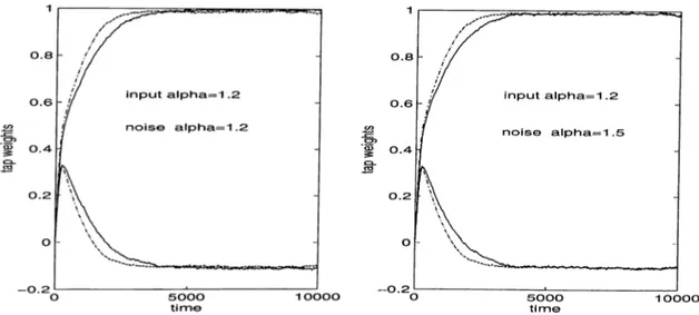
when the noise distribution has a values cis 1.2 and 1.5, respec tively. For comparison the performance under no additive ol)- servation noise is also plotted (dashed line). The A R (2) process parameters are a\ = 0.99 and a-z = —0.1... Transient behavior of the tap weight cidaptations for the NLMP algorithm of Equations (4.19) for ci = 1.2 under additive im pulsive observation noise (solid line) when the noise distribu tion has a values 1.2 and 1.5, respectively. For comparison the performance under no additive observation noise is also plotted (dashed line). The A R (2) process parameters are ai = 0.99 and
«2 = —0.1.
32
33
34
4.6
4.7
Transient behavior of the tap weight adaptations for the pro posed FLOS bcised algorithm of Equations (4.2) and (4.3) (dashed line), and the NLMP algorithm (solid line) of Equations (4.19) , for a. — 1.2 under additive impulsive observation noise when the noise distribution has a values 1.2 and 1.5, respectively. Transient behavior of the tap weight adaptations for the pro posed FLOS based algorithm of Equations (4.2) and (4.3) (dashed line), and the NLMP algorithm (solid line) of Equa tions (4.19) , for a = 1.2. The A R (2) system, with = 0.99 and tt2 = —0.1, is modeled by an AR(5) system... 4.8
4.9
Ti’cinsient behavior of tap weight adaptations for the “Momen tum” FLOS based algorithm (dashed line) of Equations (4.22) and (4.23) and the proposed P'LOS based algorithm (solid line) of Equations (4.2) and (4.3) for a = 1.1, cv = 1.2, a = 1.5, and e — 0.1. The A R (2) parameters are ai = 0.99 and ti2 = —0.1. . Transient behavior of tap weight cidaptations for the “Momen tum” NLMP algorithm (dashed line) of Equation (4.25) and the NLMP algorithm (solid line) of Equations (4.19) lor cv = 1.1, cv = 1.2, a = 1.5, and e = 0.1. The A R (2) parcuneters are fii = 0.99 cind «2 = —0.1...
4.10 The system mismatch for the “Momentum” FLOS based algo rithm (dashed line) of Equations (4.22) and (4.23) and the “Mo mentum” NLMP algorithm (solid line) of Equations (4.25) for cv = 1.2. The AR(5) parameters are «i - 0.89, «2 — —0.152, a.3 = 0.1, tt
4
= —0.197 and = 0.097... 4.11 Transient behavior of tap weight adaptations for the “ Momentum” FLOS based algorithm of Equation (4.22) and (4.23) lor a — 1.1 and cv - 1.5 under additive impulsive observation noise with cv = 1.2 (solid line). For comparison the performance under no additive observation noise is also plotted (dashed line). The AR(2) parameters are ai = 0.99 and 02 = - 0 .1 ...
35 36 39 40
41
4 1 XI4.12 Transient behavior of tap weight adaptations for the “Momen tum” NLMP algorithm of Equation (4.25) for a = 1.1 cuid cv = 1.5 under additive impulsive observation noise with a = 1.2 (solid line). For comparison the performance under no addi tive observation noise is also plotted (dashed line). The A R (2) parameters are a\ = 0.99 and a-z = —0.1 42 4.13 Transient behavior of tap weight adaptations for the “Momen
tum” FLOS based cilgorithm (dashed line) of Equations (4.22) and (4.23) and the “Momentum” NLMP algorithm (solid line) of Equation (4.25) for cv = 1.1 and a = 1.5 under additive im pulsive observation noise with cv = 1.2. The A R (2) parameters
are a\ = 0.99 and az = —0.1. 42
4.14 System mismatch for the proposed “Momentum” FLOS based algorithm of Equations (4.22) and (4.23) (left) and for the “Mo mentum” NLMP algorithm of Equation (4.25) (right). Solid line for j = 1, dashdot line for j = 3 and dashed line for j = 5. The AR(5) parameters are ai = 0.89, uz = —0.152, (I
3
= 0.1,a.., = -0.197 and as = 0.097. 43
4.15 Transient behaviour of the first tap weight for “Median” FLOS based algorithm ol Equations (4.26) (left) and for the “Median” NLMP algorithm ol Equation (4.28) (right). Also the algorithms of Equation (4.2) and (4.3) (left) and Equation (4.19) (right) with dashed tine. True value, a\ — 0.89, is plotted by the dashed
line. 44
4.16 The nonlinearity used for the input and the desired signal. . . . 46 4.17 FLOS based algorithm of Equations (4.2) and (4.3) (left) and
NLMP algorithm of Equation (4.19) (right) with (dashed) and without (solid) prenonlinearity, respectively... 46 4.18 “ Momentum” FLOS based algorithm of Equations (4.22) and
(4.23) (left) and “Momentum” NLMP algorithm of Equation (4.25) (right) by using nonlinearity, for j = 0,1,3 and 5 for the heavy solid, solid, dashdot and dashed line, respectively. 47
4.19 The s3'’stem mismatch, ||Wfc —W*||2, for the “delayed” FLOS based algorithm of Equations (4.30) (dashed line), and the “de layed” NLMP algorithm of Equation (4.31) (solid) line. The A R (2) process parameters are (q = 0.99, tq = —0.1... 48
5.1 Ti’cinsient behaviour of the tap weights for the LMMN algorithm for a =
1.2
... 535.2 The system mismatch for RLMMN algorithm (solid), the cd-gorithm of Equation (5.27) (dashdotted) ¿md Equation (5.26) (dashed) for cv = 1.2 and A = 0.9... 57 5.3 The system mismatch for RLMMN cdgorithm (solid), the al
gorithm of Equation (5.27) (dashdotted) and Equation (5.26) (dashed) for a = 1.2 and A = 0.1... 58 5.4 Transient behaviour of the tap weights lor RLMMN cdgorithm
(dashed) and the algorithm of Equation (5.28) (solid) for a = 1.2 and A - 0.1. A R (2) process parameters are = 0.99 and
U2 = -0 .1 . 58
LIST OF TABLES
4.1 Table of computation results of a for different values of N 45
5.1 A versus the convergence speed. 56
Chapter 1
INTRODUCTION
'I'iie Gaussian distribution has been by iar the most popuhir statistical distribu tion in signed processing. This distribution has been widely used to model the noise in the analysis of signals corrupted during transmission or measurement. Many theorems in the fields of communications, speech analysis, estimation and detection hcive used Gaussian noise assumption. Having no a priori in formation cibout the noise process, this is a well justified cissumption due to the “ Central Limit Theorem” [1]. The second reason that nudies a Gcuissian noise assumption attractive is its cuicdytical tractcd^ility. The filled reason is that Gaussicin processes are easy to describe, i.e., only the first two moments are sufficient to characterize a Gaussian process.
Unfortunately, there are also many phenomena in signal processing which are decidedly non-Gaussian [2]-[4]. Some examples of non-Gaussian noise are atmospheric noise [5]-[7], underwater acoustic noise [8], noise on telephone lines [9, 10], low frequency electromagnetic interference [11] cind degrcidations on aged ciudio recordings [12]. The common property of most of these type of noises is that they show impulsive behaviour, that is they produce large- amplitude outliers much more frequently than Gaussian noise. These high amplitude samples correspond to very low probability parts of the Gaussian probability density function, therefore they are not likely to be the samples from a Gaussian probability density function. This indiccites that impulsive noises can only be represented by heavier tailed probability density functions than Gaussian distribution.
Several citternpts were made in developing a statistical model lor impulsive noise [4, 5], [12]-[16]. In this thesis, we concentrate on impulsive type noise
using the statistical model of a-stable distributions developed by Nikias and Shao [17] and of e-contaminated Gaussian distributions [3]. We develop some a.dciptive filtering algorithms.
An cidaptive filter is a learning and self designing system which adjusts its parameters by a recursive algorithm to optimize some i^erformance criteria. In this thesis, robust adaptive filtering algorithms are developed for impulsive noise environments.
A brief outline of the chapters in this thesis is given below :
In Chapter 2, cr-stable distributions and some of their properties will be presented. We also give information about e-contaminated Gciussian distribu tions.
In Chcipter 3, a family of the NLMS algorithms [18] are investigated. The performance of these algorithms are examined in impulsive noise environments for system identification both theoretically and experimentally. We also study the performance under additive observation noise. We observe that they have a very poor performance in impulsive noise environments.
In Chcipter 4, we introduce a new family of adaptive filtering cdgorithms based on the Fractional Lower Order Statistics (FLOS) concept. Some proper ties of the proposed FLOS based algorithms are investigated. We also present other existing FLOS based adaptive filtering cilgorithms for impulsive noise environments and compare their performance.
In Chapter 5, we modify the Least Mean Mixed Norm algorithms using the FLOS. We investigate the properties of the LMMN algorithms in impulsive noise environments. Then the proposed family of the algorithms is investigated. Simulation studies will be presented.
In ChaiDter 6, proposed algorithms are compared and directions for the future work cire addressed.
Chapter 2
SOME HEAVY TAILED
DISTRIBUTIONS
2.1
Introduction
111 this cluipter, we introduce cn-stable distributions and e-contarninated Gaus sian distributions. We review their chcU’cicteristics and statisticcd properties. 'J'he proofs of most of the results are omitted but can be found in probability and statistics literature such as [l],[20]-[26].
2.2
o-Stable Distributions
The characteristic iunction of cv-stable distributions are given by : (j){t) = exp{zai — 7|i|^'[l + z^sign(Z)u;(i, a )])
where
tan ( i f ) if cr f 1
flog|i| ifcv = l. and
-oo < a < oo, 7 > 0, 0 < a < 2, —1 < /i^ < 1.
(
2
.1
)(2.2)
(2.3) In the above expressions, a is the location parameter, 7 is the dispersion, ¡3 is the index of skewness and cv is the charcicteristic exponent. When fi = 0, tlie
distribution is called symmetric a-stable (SaS). The chariicteristic exponent, cv, controls the tails of the distribution. For 0 < o; < 2, the distributions have algebraic tails which are significantly heavier than the exponential tail of the Gaussian distribution. The smaller the Vcilue of the a, the heavier the tails of the distributions. When cv = 2, the relevant stable distribution is Gaussian. Gauchy distribution is also an a-stable distribution with a = 1 and ^ = 0.
The a-stable distributions are called standard when a = 0 and 7 = 1. Then, one can see that if X is an a-stable rcindom Vciriable with parameters a, fJ, 7 cind a then {X — a)f'ya is standard with characteristic exponent cv and skewness p.
By taking the inverse Fourier transform of the chciracteristic function, it is easy to show that the standard stable density function is given by
1 rco
i
f(x ; cv, 1^) = - e x p ( - i " ) cos[xi + /3t°'w(t, a)]dt.
IT Jo
(2.4) Note that /(;c; cv, ¡3) = f { —x] a, —(3)· It can ivlso be shown that the probability density functions of the cv-stable distributions are bounded cirid have derivatives of arbitrary orders [21]. Unfortunately, no closed-form expressions exist for the general cv-stable density and distribution functions, except for the Gaussian (cv = 2), Cauchy (cv = 1,(3 = 0), and Pearson (cv = |,/3 = —1) distributions [26]. But power series expansions of their density functions are available. The stcuidcird cv-stable density function can be expanded into convergent power series as follows [1], [21, 22], [26, 27]. For .t > 0,
¿ X r . i G G - r i « * : + [ 7 ( a + i)j fo>· 0 < o < 1 for 1 < cv < 2 ,/'(» ·■ ;
(З) =
< where+ D p ) sin [g(a + {)
Г] = ^ tan(7rcv/2). /1 1 r = (l + r/^) = —(2/7t) arctan(7). The r is the usual gamma function defined byroo
r(.T) = / t^-^-^dt. Jo
In particular, the standard SaS density function is given by
k-na (2.5)
(2.6)
(2.7) (2
.8
)Ш =
7Г(.Т7^ +1) ro' ^ k = 0 2kl ' тга 1 2fc+lV„2fc a for 0 < CV < 1 for cv = 1 for 1 < cv < 2 for a = 2.The standard SaS density functions for a few values of the characteristic exponent a are shown in Figure 2.1. Observe that ScvS densities hcive many features of the Gaussian density. They are smooth, unimodal, symmetric with respect to the median and bell-shaped. A detailed comparison between the standard normal and SctS density functions shows that non-Gaussian stable density functions depart from the corresponding Gaussian density in the fol lowing ways. For small absolute values of x, the SaS densities are more peaked than the normal. For some intermediate range of |.r|, the ScvS distributions have lower densities than the normal. Most importantly, unlike the Gaussian density which has exponential tails, the cv-stable densities have algebraic tails [23]. Thus, the SaS densities have heavier tails than the Gaussian density [see Figure 2.1 (b)].
2.2.1
Basic Properties of a-Stable Distributions
Two of the most important properties of the cv-stable distributions are the Stability Property and the Generalized Central Limit Theorem. They are re sponsible for much of the appeal of the stable distribution as a statistical model of uncertainty.
The stability property is actually a defining characteristic of cv-stable dis tributions.
Theorem 1 (Stability Property) : A random variable X is cv-stable if and only if lor any independent random variables X j, X-2 with the same distribution as X , and tor arbitrary constants cii, a-2, there exist constants a, and b such that
ayXi -)-
02
X2
— a X -|- b (2.9) where the notation X = Y means that X iincl Y have the same distributions. By using the characteristic function of the a-stable distributions, one can easily sliow a more general stcvtement : if X y ,X2
,...,X n are independent and liave cv-stable distribution functions with the same (a,/3), then all the linear corn- l)inations of the form are a-stable with the same parameters cv andAs a conseciuence of the stability property, it can be shown that cv-stable distributions are the only possible limit distributions for sums of independent identically distributed (i.i.d.) random variables. This is known as the Gener alized Central Limit Theorem and is formally stated as follows [20]:
Figure 2.1: Density functions of SaS distributions for different values of char acteristic exponent a :(a) the overall densities and (b) the tails o f the densities.
Theorem 2 (Generalized Central Limit Theorem) : X is the limit in distri bution of normalized sums of the form
Sn = (^1 + ··· + X\)/an — bn (2.10) where X i , X
2
, are i.i.d. and a„ ^ oo, if and only if X is stable.In ¡^articular, if Xi's cire i.i.d. and have finite variances then the limiting distribution is Gaussian. This is of course the result of the ordiiiciry Centred Limit Theorem.
The main cause of different behaviours of the Gaussicui and «-stable dis tributions is their tails. It can be shown [28], [29] that for «-stable random variable X with zero location parameter and dispersion 7,
lirn i"P(|A"| > t) = 'yC(a)
¿—»•CO (2.11)
where C (a ) is a positive constant depending on « . The «-stable distributions hewe inverse power (i.e. :algebraic) tails while Gaussian distribution has expo nential tails. This fact shows that the tails of «-stable distributions are much heavier than the tails of the Gaussian distributions.
Equation (2.11) has an important consequence thcit the second-order mo ment of cv-stable distributions, except for the limiting case « = 2, does not exist. This can be written as in the following proposition [17]:
Proposition : Let X be an «-stable random variable. If 0 < « < 2 then E[|A:n = 00, if p > « (2.12) and
If « = 2, then
E [|X f] < 00, if 0 < p < « .
E[|A"H < 00, for all p > 0.
(2.13)
(2.14)
Therefore, «-stable distributions have no finite first or higher-order mo ments for ( ) < « < ! ; they have finite first-order moments cind all the fi’cictional moments of order p for 1 < « < 2 where p < « ; and all the moments exist for « = 2. Note also that «-stable distributions have infinite varicinces.
2.3
Symmetric a-Stable Random Variables
and Processes
A real random variable (r.v.) X is ScvS, if its characteristics function is of the form :
= exp{iat - 7|i|"} (2.15) where 0 < a < 2 is the characteristic exponent, 7 > 0 is the dispersion, and
—00 < a < 00 is the location parameter. When a = 2, X is Ga.ussian and when a = 1, AT is Cauchy.
2.3.1
Fractional Lower-Order Moments
Although the second-order momerii of a So;S random variable with 0 < cv < 2
does not exist, all the moments of order less than cv do exist and are called the fractional lower-order moments or FLOM’s. The FLOM’s of a ScvS random variable can be easily found from its dispersion and characteristic exponent as follow.
Theorem 3 : Let X be a ScvS r.v. with zei’o location pcvrarneter and disper sion 7. Then,
E[|V|»| = C(
p.
q)7"/“
(2.16)
for ( ) < / ) < cv, where
C(p, cv) = 2P+iF(2± i ) r ( _ p / « ) (2.17) cv7rF(—p/2)
depends only on cv and p, not on X . In this expression F is defined in (2.8). 'I'his important result was first proved by Zolotarev using the Mellin-Stieljes transform [30]. Cambanis and Miller rediscovered [31] it by using a property of the characteristic function derived in [32]. An elementary proof of the theorem using basic properties of the gamma function is given in [17].
A fundamental difficulty in stable sigiicil processing with lower-order mo ments is that the tools of the Hilbert space theory are no longer applicable. yMthough the linear space of a Gaussian process is a Hilbert space, the linear spa.ce of the cv-stable distributions is a Banach space for 1 < cv < 2 and only a metric space for 0 < cv < 1 [17], [33].
2.4
^-contaminated Gaussian Distributions
The e-contaminated Gciussian mixture density has the probability density func tion of (1 — e)N {0, + eA^(0, Acr^). This family of the distribution is chcu’cic-tcrized by the mixing parameter e which is the fraction of the contamination. The outliers of the distribution are also Gaussian but have A times the varicuice of the dominant distribution, resulting in an impulsive behaviour.A typical realization of e-contaminated Gaussian distribution is given in the following figure. In this figure we take e = 0.1, A = 10 and cr^ = 1.
-15
0 100 200 300 400 500 600 700 800 900 1000 time
I'’igure 2.2: A typical realization of e-contaminated Gaussian mixture.
2.5
Conclusion
In this chapter, we briefly review some heavy tailed distributions, namely cv- stable distributions and e-contaminated Gaussian distributions. I'hrough the thesis we use these two chisses of distributions for modeling impulsive noise environments.
Chapter 3
A FAMILY OF NORMALIZED
LEAST MEAN SQUARE
ALGORITHM
3.1
Introduction
Normalized Least Mean Square (NLMS) algorithm is first developed by Naguino and Noda [36] cind Albert cuid Gardner [37] independently. This a.l- goritlmi is cdso Ccilled the projection algorithm [35]. In [36], ci modified version of the NLMS [36] is introduced. Properties of the NLMS algorithm are studied in [34] and in [18] a genercxlized family of the NLMS algorithms are presented.
In this chapter, we first review the above algorithms with some of their properties. Then using the adaptive filtering configuration of Figure 3.1 we investigate the performance of the NLMS type algorithms in impulsive noise environments.
3.2
NLMS Algorithm
'I'lie NLMS algorithm of [36] and [37] has the following update eqiuition : (ik
W w = W t + , . - Xt Z^m
=0
'^k—rn(3.1)
where W k = [iOo,k---WM-i,k]'^ are the tap weights of the achiptive filter at time
k, X^. =
[xk---Xk-M+i]'^ are theM
samples of the input data in filter memory at time k, tk = dk ~ is the error between the adaptive hlter output and the desired signal dk, and ¡i is the step size which should be appropriately determined.A variety of the theoretical results for NLMS algorithm such as conditions for convergence, rates of convergence and the effects of errors due to digital implementation of the algorithm are given in [38, 39].
Figure 3.1: Adciptive filtering block diagram
3.2.1
Performance of NLM S Algorithm in Impulsive
Noise Environments
Consider an AR(L) a-stable process, defined as follows.
Xk = X ] a-iXk-i + Uk
i = i
(3.2)
where Uk is a symmetric a-stable (SaS) sequence of random variables. The random variable Xk is cilso symmetric a-stable (SaS) with the same parameters as Uk [17], [40] if {a,·} is an cibsolutely surnmable sequence.
The NLMS algorithm of Equation (3.1) is used to identify ¿m AR system driven by cin i.i.d. SaS rcuidom process, Uk, with three different values ol the a parcuneter as well as e-contaminated Gaussian noise. AR(2) process has the parameters ai = 0.99 cuid (I
2
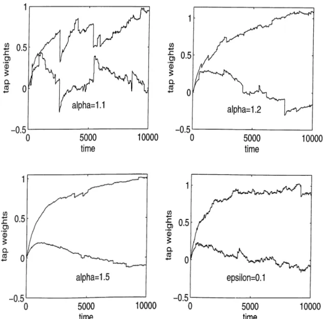
= -0 .1 . The tap weight values versus time |)lotscire given in Figure 3.2. We used cv = 1.1, 1.2 and 1.5 values for the ScvS pro cess and standard Gaussian random process N { 0 ,1) contaminated by cuiother Gaussian process N { 0 ,10) with contamination rate e = 0.1. As it can be seen from Figure 3.2, the performance of the algorithm is far from satisfactory. We repeat the experiment under additive observation noise. For various a values and c-contaminated Gaussian random processes, the performance is seen in Figure 3.3. Again, we conclude that the performance is far from satisfactory.
Note thcit in this thesis cdl the simulations are obtained by averaging 100 independent trials of the experiment and for ecich trial, a different computer realization of the process Uk is used.
3.3
A Modified NLMS Algorithm
'I'he NLMS cilgorithms requires a minimum number of one additiomil multipli cation, division and addition over the usiuil LMS algorithm [41], which has the following update equation :
= W ic + iiei^X.)·, (3.3)
to implement for shilt-input data. Even so, the multipliers required for the algorithm update niciy still be prohibitive in certain high-data-rate applications. In these situations, it is useful to determine modified versions of the NLMS aigorithm of Equation (3.1) while reducing the computation per iteration. One such modilied algorithm, first suggested by Naguino and Noda [36], is :
W k + i ^ W k + i-f, e-k
\xk-r -sign(X;t)·
(3.4)
This update is similar to thcit of Equation (3.1) but allows the nonlinear trans formation of the input data vector elements.
3.3.1
Performance of the Modified NLM S Algorithm
in Impulsive Environments
'fhe same experiment of Figure 3.2 is performed for the modified NLMS algo rithm of Equation (3.4). The plot is in Figure 3.4. The concluding remark is again that this algorithm is unsatisfactory in impulsive noise environments.
3.4
A Family of NLMS Algorithms
ill [18] a fcimily of NLMS cilgorithrns is derived with the motivation of the N LMS and the modified NLMS algorithms mentioned above. The update equation is given l:)y :
Wfc+i = W , + ^cekF,{Xk)
(3.5) K i x n j i \xk-i\'^ ^sign(a;fe_^) Em=0 if 1 < (/ < oo (3.6) ~^i~n \[q oowhere [T]/.)]; denotes the element of the vector-valued function /'],(.), n is any one of the integers 0, — 1 such that = maxo<j<M-i |·'í'·^-,■|, and
8
j is the Kronecker delta function. For q = 2, this algorithm reduces to the NLMS cdgorithm of Equation (3.1) and for q = 1, this update reduces to the modified NLMS algorithm of Equation (3.4). For = 1, this algorithm is shown to be the solution of the following optimization problem [18] :minimize ||W/;+i dk W ,k\\p subject to W f + i X , ^ 0 (3.7) (3.8) where |].]|p denotes the Lp norm, and p satisfies the Holder inequality l/p 4- l/q = 1. Therelore, the adaptation algorithm of Equations (3.5) and (3.6) provides the minimum change in an Lp-norm sense of the tap weights to ex actly satisfy the filtering relationship between the input data and the desired response at time A:, similar to a projection in the / /2-norm case. Investigating the algorithm ol Equations (3.5) and (3.6) for q = oo, that is for //i-norm case, the update equation takes the following form:
■Wг,k+^
Wi,k + if maxo<j<M-i \Xk-j\
(3.9) otherwise.
1 Wi,k
In this update equation, the maximum absolute value of the input data vector |:i.·/,;_;] = rnaxo<;<j\//-i l-'i-’i'-il ii’ supposed to be unique. In the case of being not unique, a single filter tap weight of the set {wi^k ■ |·'í'■A:-¿| = maxo</<y\/f-i|.'i'’A:-i|} is chosen randomly for updating. Therefore the only filter tap weight changed a.t time k is a tap weight associated with an input sample that has the largest absolute value of all input data samples currently in the filter memory.
3.4.1
Derivation
In this section we review the derivation of [18] in which it is shown thcit the algorithms of Equations (3.5) and (3.6) solve the optimization problem in Eqiui- tions (3.7) and (3.8). This derivation follows a similar derivation of [42] for the modified NLMS cilgorithm and uses the following theorem :
Theorem : Let
A
be a nonzero vector contciined in the vector space cuid b be a scalar quantity. Then, the minimum Lp-norm solution vector Z to a consistent linear equationZ
= b is given byZ = 6T’ (A)
(3.10)
where the vector function Fq(.) is given by Equation (3.6).
Proof : Let ai and Zi denote the T'' elements of the vectors
A
andZ,
respectively. Then
M-l
= I a,z,\ < ||Z||„||A|
¿=0 (3.11)
where the inequality follows from the Holder inequality with l/p +
1
/q =1
. Thus, for the nonzero vector A , we haveIM
Consequently, the Ibllowing inequality holds :
miriA'rz=6||Z|| > \ b \
iiA ii;
(3.12)
(3.13)
Let Z be a solution vector to the equation A^ Z = b. Note that Z is not unique but that it satisfies
Pl l p > minAï’z=6||Z||p for all ||Z|| in R ^ . Now, let
Z = bF ,(A ). It can be seen tluit for 1 < ç < oo
|Z||„ = |i>l
E
_ ii-i / E S i t M T ! ! '
i/p
iiAii;PI
1IA|I, I IIAII
7(3.14)
(3.1.5)
(3.16)
14Using the relationship p — q/{q - 1), the term inside the parenthesis of (3.16) can be shown to be equal to one. Thus, from (3.13) and (3.16), we have
minATz=b||Z|| . (3.17)
Considering the case (p = ! , < / = oo), it is found from (3.13) and (3.16) that
|z||x = |i>l
l|A|L
= minATz=6||Z||i. (3.18)Therefore, Equation (3.10) follows.
To see how the theorem enables the solution to the problem posed in (3.7) and (3.8), assign Z = Wr.+i — W^., A = X^.., and b = ek. Then, Irorn the definition of the error we have
('k, = d t - x l W t = ( 4 - x i 'W t + .) + x i ( W i + , - W t).
(3.19)
If the constraint in Eqiuition (3.8) is satisfied, then from the assignments of Z, A , and bX iiW k + i - W k ) = Ck A^ Z = b (3.20) and thus, the optimization problem in Equation (3.7) and (3.8) is the sai a.s the minimizcition of ||Z||p subject to A ^ Z = b. Therefore, from Equa.ti (3.17), the optimum update for W k is given by (3.5) and (3.6).
ne ion
3.4.2
Variance Analysis for Impulsive Environments
in this section we will show that :
E [| | W ,.+ i-W ,| 0 = oo (3.21)
for the family of the NLMS algorithms presented above, for both finite and infinite q.
Fiiiite q case : Equation (3.5) and (3.6) can be written for each sample of W i, as follows : foign(aifc_/) Щ,Ш - '^i,k + /iCfc M -l I |, l^rn= 0 (3.22) cind
E[(r0i,i;+1 - Wi^kY] = p^E ЩХк-Л
-1 \
(3.23)
If the cilgorithrn converges at steady state, it can be assumed that the error, and the samples of the random process are uncorrelated. Thus the right hand side of the hist equation can be written as ;
17-1 2-jm=0 \^^k-rn\ , = ^ı^E[e,^]E \xk~. 17-1 I 17 ^m=0 , (3.24)
In the following, we will show that E[e^.^] in Equation (3.24) is infinite and the hist expectation is strictly positive for at least one value of i, 0 < i < M — 1., 'This way, we will be able to conclude that the left side of Equation (3.24) is infinite for at least one value of z, hence the claim in Equation (3.21) is true. For this purpose, let us investigate the last expectation for the index j , which js chosen such that — maxo<y7i<^//—i Then, we have
\xk-j\7 - 1 > 17-1 1 E;]f=o
k w r "
(3.25) implying.E
17-1 > ^ E - M2 P-’fc- (3.26)Using .lensen’s inequality for the last term we obtain :
M2
E
Lh^T-il J
>(:i.27)
where the right hand side is zero since E[|a:fc_j|^] = oo. So, we can say that the second expectation term in the right hand side of Equation (3.24) is strictly greater tlian zero.
As lor the first expectation term, E[cfc2], it includes some linear combina tions of E[xk-i^]· Knowing that the samples of are ScvS random variables, it is clecir that E[eA,·’^] has an infinite value. Therefore :
- Wj^kf] = oo (3.28)
implying
E|||Wi+,-Wi|0
= (X ). (3.29)Infinite q case : In this Ccise, Equation (3.9) can be rewritten iis :
Wi fc T : if I^A:—i’l 1 m i
Wi^k otherwise
16
and
E [| | W ,+ J -W ,| a = ;«^E 4 (3.31)
Agcun a.ssuming that the error and the samples of the input vector are uncor related and the system converges, this last equation can be expressed as
1
Xk-(3.32) Using the Jensen’s inequality, [44], the second expectation term in the right hand side of Equation (3.32) may be written as :
Since E[xi;-i^] = oo, we can say that the left hand side of Equation (3.33) is strictly greater thcin zero.
Similar to the finite q case, E[ek^] is infinite since it includes some linear combinations of E[xk-i^\· Therefore, we can conclude that
E[||W ,+i-W ,||^] = oo. (3.34)
It can be also shown that in the case of Gaussian excitation and a-stable observation noise, i.e., Xk is a Gaussian AR sequence and (4 = + Hk where Uk is «-stable, the vciriance of the update term of Equation (3.22) and lii|uation (3.30) is not finite, either.
3.4.3
Performance Analysis of the Family of NLM S A l
gorithms in Impulsive Environments
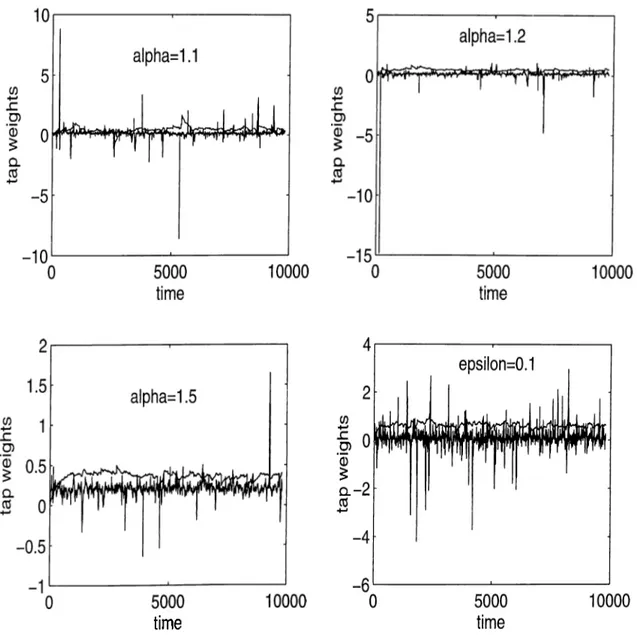
VVe repeat the same experiment tor the family of the NLMS algorithm of Equa tions (3.5) find (3.6) cis in Section 3.3.1 for a particuhir value of q and see from the Figure 3.5 that this algorithm is also far from satisfactory when the «-stable distributions are used.
3.5
The Family of NLMS Algorithms with
Variable Step Size
'I'he performance of the family of NLMS algorithms is inq:)roved lor the Gaus sian environments using a variable step size, [43] instead of /i in Equation
(3.5). The variiible step size ¡Xk is :
l·>■k = -\- ptk^k-\.F{'X.k-\Y'Kk where p is a. convergence parameter for the step size.
(3.35)
3.5.1
Derivation
In this subsection, we review the derivcition for pk, [43]. In [43] the update equation is considered in a more general form, i.e..
W k + i = W k + p k f(ek )F (X k ). (3.36) Following the stochastic gradient-descent procedure as in [45] and [46], it can be written
— l^k—i P c ' d(t>{ek)
dpk-i (3.37)
The function </>(.) denotes the relevant cost function to be minimized. Also d(j){ek) d(j){ek) dck
^Pk—l ^^k ^Pk—\
Following the notation in [47], ¡{dk) = d(j){ek)/dek and putting = Wk- i + Pk-if{ek-y)FiXt,_,)
into the expression oI Ck ,
e , = dk - W k - i X k - P k - i f { e k - i ) F ( X k - , f X k is obtained. Thus, we get
(3.38)
dck
dpk-i = - f i e k - i ) F i X k - i y X k .
Combining (3.37), (3.38) and (3.41) yields the step size update as
p , = P k - i + p f { e k ) f { e k - i ) F { X k - , f X k .
(3.39)
(3.40)
(3.44)
(3.42)
Since in our case /(e^ ) = ek, the last form of the step size is as given in 1'kiua.tion (3.35).
3.5.2 Performance of the Family of the NLM S A l
gorithms with Variable Step Size in Impulsive
Noise
'I'lie Scune experiment of the Section 3.4.3 is performed agcun. As can be seen from Figure 3.6 the performance of the algorithm is unsatisfactory in the case of o'-stable distributions. This result is also obvious from the fact that the expected value of the variable step size of Eqiuition (3.35) is infinite in the case of «-stable distributions.
3.6
Conclusion
In this cha]>ter we review a family of NLMS algorithms. The performance of the algorithms are cissessed in impulsive noise environments. The obtained |)lots are far from scitisfoctory. The degradation is also shown theoreticcUly by finding the vciriance of the update term as infinite by using cv-stable random processes. After all, it is clear that we need to develop some robust algorithms for impulsive noise environments.
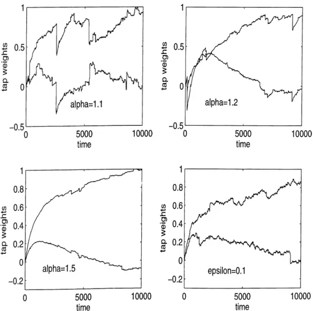
Figure 3.2: Transient behavior of tap weight crdaptations for the NLMS algo rithm of Equation (3.1) for a = 1.1, a = 1.2, a = 1..5 and e = 0.1. The AR(2) process parameters are ai = 0.99 and a2 = —0.1.
time
time
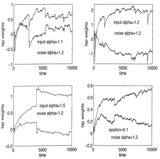
Figure 3.3: Transient behavior of tap weight adaptations for the NLMS al gorithm of Equation (3.1) for a - 1.1, a = 1.2, cv = 1.-5 and e = 0.1 under additive observation noise whose a = 1.2. The AR(2) process parameters are
0,1 = 0.99 and «2 = —0.1.
10000
time
time
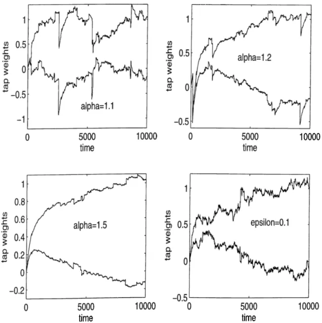
Figure 3.4: Tran.sient behavior of tcip weight adciptations for the inodified NLMS algorithm of Equation (3.4) for a = 1.1, a = 1.2, a = 1.5 and e - 0.1. The AR(2) proce.ss parameters are «j = 0.99 cind 02 = —0.1.
time
Figure 3.5: Transient behcivior oi tap weight achiptations for the family of the NLMS algorithm of Equations (3.5) and (3.6) for a = 1.1, a = 1.2, rv = 1.5 and e = 0.1. The AR(2) process parcirncters are ai = 0.99 and «2 = -0 .1 .
time
Figure 3.6: Transient behavior of tap weight adaptations for the family of the NLMS algorithm of Equations (3.5) and (3.6) with variable step size of Equation (3.35) for a = 1.1, a = 1.2, a = 1.5 and £ = 0.1. The AR(2) process parameters are a\ = 0.99 and a
-2
— —0.1.Chapter 4
FRACTIONAL
LOWER-ORDER STATISTICS
BASED ALGORITHMS
4.1
Introduction
The well-known NLMS algorithm is based on a second-order cost function. Therefore it exhibits poor performance under cv-stable noise. We robustify this cdgoritlirn using the Fractional Lower Order Statistics (FLOS). In this chapter, proposed adaptive algorithms utilize fractional moments and correlations.
In the following section, the proposed FLOS based lainily of cilgorithms and some of their properties are investigated. In Section 4.3 and 4.4 some existing FLOS based adai^tive filtering algorithms for cv-stable distributions are reviewed. Following these, simulation results are presented. The perfor mance of these algorithms are investigated for systems with unknown orders in Section 4.5. In Section 4.6 “Momentum” FLOS based adaptive algorithms are proposed with relevant simulations. In Section 4.7, “ Median” FLOS based adaptive algorithms are introduced and in Section 4.8, we modify the FLOS based algorithms using a prenonlinearity at the input and the desired signal. “ Delayed” FLOS based algorithms are presented in Section 4.9. Extensive simulation studies are also presented.
Let us introduce the following notation [17]. For any two real numbers .2
^<y> A
where sigri(.) is the signurn function.
a n d y > 0 a s :
4.2
Proposed FLOS Based Algorithm
As it is discussed in Section 3.4.2, the variance of the update term of the algorithms presented in Chapter 3 is not finite in impulsive environments. In order to achieve a finite variance, i.e.,
E ( | | W i + , - W t i a < c »
(4.1)
we modify the algorithms of Chapter 3 using Fractional Lower Order Statistics (FLOS) concept.The fractional lower-order moment (FLOM) of the error, E[|eA;|*], is finite for Q < h < Oi. Based on this observation we define the following update eqiuition [51], [52], [53] :
= W , + ye,<“>F,(X,.)
(4.2)E„,=o
b"
if (7 = 00 ^oa if 2 < (7^ < oo (4.3) ‘^k-nwhere [Fg(.)]i· denotes the element of the vector-valued lunction F',(.), q satisfies the relation 1 /a + l /y < 1 . The FLOS parameter a > 0 obeys the following inequality :
a < 1/2. (4.4)
Also, it is eclsy to check that actual weights form a stcitionary point of the iterations. Hence, it is expected that the above class of algorithms which we Ccdl FLOS based will have better performance than those in Chapter 3, in impulsive environments.
In the following we will prove Equation (4.4) both for finite and infinite q
Cci.se.
by :
Finite q case : The update equation of the FLOS based algorithms is given
_ , ^^“sign(.^A,-0
W i,k + i - Wi,k + iiC k ^ M- 1 1 — —
Z-^m
=0
(4.5)
for each sample of the weight vector W ^. Equation (4.5) implies that : / I i a i „ \
n2i ,2i
E[('u;iy-+1 - Wi^k) ] = /2 E k;ci (4.6)
which Ccin be written as :
^i^E Y'M-l I I'J ¿^m
=0
\'^k-m\/^^E[|e,r“]E f o ’ f c - i E M -1 L·, I
m=0 \^k—m\ (4.7)
by assuming that the error is uncorrelated with the past samples, Xk-i , of the input at steady state.
To licive a finite value of the first expectcition term in the right hiuid side, we should have the following inequality:
a < a/
2
. (4.8)For the second expectation term of the right hand side of Equation (4.7), let |a:A,._/| = m a x o < T O < M - i t h e n the term inside the expectation can be written as :
l^k—i1(7-1)“ < 1(7-1)“ < Ir, .|('i~L“
[70
1
\xk-rnr ~ \^k-rnr
From here, we have to find the value of a satisfying the following:
1
(4.9)
E
k k -j \2a
<
00
. (4.10)It is shown in [61] that the ¡property given in Equation (2.13) is cdso valid for the interval —1 < p < « . Therefore the condition in Equation (4.1) is satisfied when
a < 1/2. (4.11)
Since the value of a is in the interval [1,2), in the applications of adap tive filtering for impulsive environments, taking the simultaneous solution of
Equation (4.8) and (4.11) we get the condition for a as in Equation (4.11), i.e., a < 1/2 having :
E[||W,+a-W,||^]<oo.
(4.12)Infinite q case : The update equation of the FLOS based ¿ilgorithm can be rewritten as :
4" Xk—: l^/s—¿1 1 7« I
I0i,k+1 =
Wi^k otherwise.
(4.13)
So we consider for the analysis oidy the value of i for which |.rfc_,| = inciXo<77x<M-i|a;fc-ml- Then, we may write
|2fi
(4.1<1)
.\Xk-i\ 2a
Agciin cissurning that the error and scimples of the input vector are uncorrelated cUid the system converges, this last equation can be expressed as :
E[||W7,+i-Wj||‘ J = ,.^E(|e,r|E 1
. — t
12a (4.1.5)
To have a finite value for the E[|ei,.p“] we must have the condition of Equation (4.8) for a. Following the same arguments as in finite q case, for the second expectation term we have for a again the condition of Equation (4.11). Taking the intersection region, we obtciin a < 1/2 for having
E[||W,+i-W,.||J<oo.
(4.16)4.3
Least Mean-p Norm (LM P) Algorithm
The first of the FLOS based adaj^tive filtering algorithms for impulsive noise environments is called Least Mean-p Norm (LMP) [17] algorithm with the following update equation :
W ,+ i =
The cost function of this algorithm is given by,
.h = E[|ein = E [|* - WlXtf]
where 1 < p < cr.
(4.17)
(4.18)
There is no closed-form solution for the set of the coefficients minimizing Equation (4.18). But knowing that Jk is convex, a stochastic gradient method to solve the coefficients as in Equation (4.17) Ccui be used. The algorithm in Equation (4.17) is called Least Meiin Absolute Devia.tion (LMAD) when p =
1
. The LMAD is actually the familiar signed LMS algorithm, although it is derived in a different context.4.4
Normalized Least Mean-p Norm (N LM P)
Algorithm
With the motivation of the NLMS algorithm, recently LMP algorithm is nor malized giving the Normalized Least Mean p-Norrn (NLMP) [3.3] cdgorithm by the Ibllowing update equation ;
W ,+ i = W k + P, -Xyt lor 1 < p < a P O i f + A'^* ^ ^
where p, A > 0 are appropriately chosen update parameters. When p = 1 tlie algorithm in Equation (4.19) is called Normalized Least Mean Absolute Deviation (NLMAD) [33], having the following update equation:
sign(cfc)
W ,+ i = W k + p- -X i (4.20)
|Xa-||i + a·
The NLMP algorithm is shown to outi^erforrn the other existing algorithms when cv-stable distributions are used, [33]. Therefore, during the simulation studies we will only consider the NLMP algorithm and the algorithm that we propose in Section 4.2.
4.4.1
Simulation Studies
In Figure 4.1, the system identification problem of Chapter 3 is considered. A comparison study is performed for the proposed FLOS based algorithm ot Equations (4.2) and (4.3) and the NLMP cdgorithm of Equation (4.19). The same comparison study is made on Figure 4.2 for an AR(3) process with coel- ficients ui = 0.99, U
2
= —0.152, = —0.097.In Figure 4.3 the system mismatch, [50], ||Wyt — W*||2, where and W * are the current tap weight and the optimal solution vectors, respectively, of the AR(3) process defined above versus time plots are given lor both algorithms.
In Figure 4.4 the proposed FLOS based algorithm is investigated under additive impulsive observation noise with the same AR(2) process as above. The degradation of the algorithm is seen from the plot clearly.
In Figure 4.5 the degradation of the NLMP algorithm under additive im pulsive observation noise is investigated with the same AR(2) process as in Figure 4.1.
In Figure 4.6 a comparison study under additive impulsive noise is plotted for the proposed FLOS based cilgorithm and the NLMP cilgorithm. From this plot it is seen that they have comparable performcince.
All the plots are obtained by 100 independent trials and to get a fair com parison between the algorithms, the step size of the algorithms are adjusted so tlicit the stecidy state Vciriances of the tap weights are equal.
time
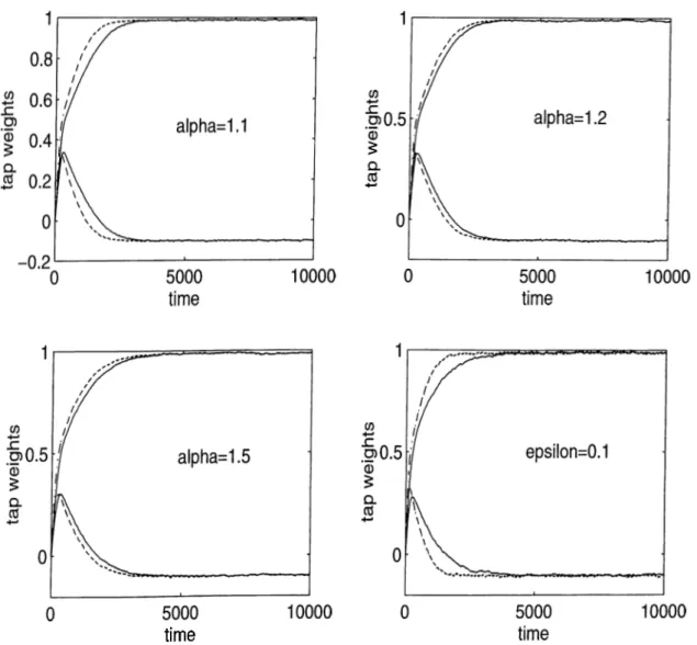
Figure 4.1; Transient behavior of tap weight aclaptcitions for the proposed FLOS based algorithm (dashed line) of Equations (4.2) and (4.3) and the NLMP algorithm (solid line) of Equation (4.19) for cv = 1.1, cv = 1.2, rv = 1.5 and £ = 0.1. The AR(2) process parameters are iq = 0.99 and a
-2
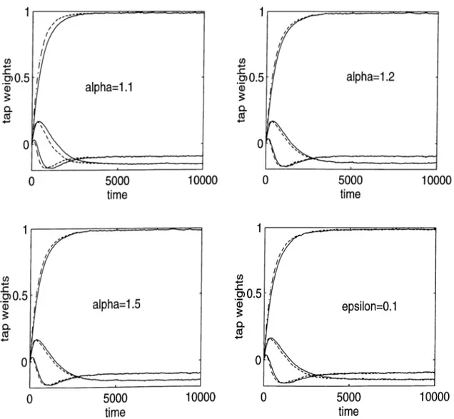
= —0.1.Figure 4.2: Transient behavior of tap weight adaptations for the proposed FLOS based algorithm (dashed line) of Equations (4.2) and (4.3) and the NLMP algorithn:! (solid line) of Equation (4.19) for cv = 1.1, cv = 1.2, a — 1.5 cind e = 0.1. The AR(3) process parameters cire ai = 0.99, a
2
· —0.152 and aa = -0.097.time
Figure 4.3: The system mismatch, ||Wfc+] — versus time is plotted for the proposed FLOS based algorithm (dashed line) of Equations (4.2) and (4.3) and the NLMP algorithm (solid line) of (4.19) for a = 1.1, a; = 1.2, cv = 1..5 and e = 0.1. The AR(3) pcirarneters are (q = 0.99, a-i = —0.152 and (¿3 = —0.097.
Figure 4.4: Trcinsient behavior of the tap weight adaptations for the proposed FLOS based algorithm of Equations (4.2) and (4.3) for cv = 1.2 under additive impulsive observation noise (solid line) when the noise distribution has tv values as 1.2 and 1.-5, respectively. For comparison the performance under no additive observation noise is cdso plotted (dcished line). The AR(2) process parameters are a\ = 0.99 and U2 = —0.1.
Figure 4..5: Transient behavior of the tap weight adaptations lor the NLMP cdgorithm of Equations (4.19) for a — 1.2 under additive impulsive observation noise (solid line) when the noise distribution has cv vidues 1.2 and 1..5, respec tively. For comparison the performance under no additive observation noise is also plotted (dashed line). The AR(2) process parameters are ai = 0.99 and «2 = -0 .1 .
Figure 4.6; Transient behavior of the tap weight adaptations for the proposed FLOS based algorithm of Equations (4.2) and (4.3) (dashed line), and the NLMP algorithm (solid line) of Equations (4.19), for a = 1.2 under additive impulsive observation noise when the noise distribution has a values 1.2 and 1.5, respectively.
4.5
Performance of the FLOS Based Algo
rithm for Systems with Unknown Orders
In practice, there may be some systems with unknown order. In this section, we try to see the performance of the proposed algorithm of Equations (4.2) and (4.3) cind the NLMP algorithm of Equation (4.19) when the order of the system is unknown.For this purpose, we generate the AR(2) SctS process with a = 1.2 and iii = 0.99 and U2 - —0.1 that we used before. Then we try to find the 5 tap weight FIR filter for this system. In Figure 4.7, we plot the transient behaviors of these 5 tap weights for both of the algorithms and see their steady state values as follows : ai = 0.9858, (I
2
= —0.0956, (I3
= —0.0047, a.i = 0.0014 and «5 = —0.0030. As it is seen from these results «3, 04 and as are so siruill that they can be neglected, i.e., the system can be thought as a second-ordertern.
Figure 4.7: Transient behavior of the tap weight adaptations for the proposed FLOS based algorithm of Equations (4.2) and (4..3) (dashed line), and the NLMP algorithm (solid line) of Equations (4.19), for cv = 1.2. The AR(2) system, with ai = 0.99 and <t2 = —0.1, is modeled by an AR(5) system.
4.6
“Momentum” FLOS Based Adaptive Al
gorithms
The algorithms presented in this duq^ter until now are all based on the in- stantcuieous value of the gradient vector. When the sigimls are Gaussian cind stationary, ignoring the past values and considering just the values of the gradi ent vector at time k for evaluating the coefficients at the step, is a reasonable approximation [49]. In impulsive noise environments, the current observation iriciy be an outlier and the corresponding update term may be useless. There fore the use of past values may provide robustness cuid improve convergence speed.
In this section, with the motivation of “Momentum” LMS algorithm [54], in addition to instantaneous value of the gradient vector, we deal also with some of its past values. By doing so, we expect to accelerate the algorithms.

![Figure 4.3: The system mismatch, ||Wfc+] — versus time is plotted for the proposed FLOS based algorithm (dashed line) of Equations (4.2) and (4.3) and the NLMP algorithm (solid line) of (4.19) for a = 1.1, a; = 1](https://thumb-eu.123doks.com/thumbv2/9libnet/5999840.126222/49.966.167.801.157.754/figure-mismatch-versus-plotted-proposed-algorithm-equations-algorithm.webp)