Estimate the yield curve for sovereign bonds in Turkey and forecasting Turkish economy from the shape of yield curve (2005 - 2018)

KADİR HAS UNIVERSITY

SCHOOL OF GRADUATE STUDIES

PROGRAM OF FINANCE AND BANKING

ESTIMATE THE YIELD CURVE FOR SOVEREIGN BONDS IN TURKEY

AND FORECASTING TURKISH ECONOMY FROM THE SHAPE OF

YIELD CURVE (2005 - 2018)

TEOMAN SAMET TEMUÇİN

ADVISOR: PROF. DR. NURHAN DAVUTYAN

SECONDARY ADVISOR: ASS. PROF. DR. SABRİ ARHAN ERTAN

PHD THESIS

ESTIMATE THE YIELD CURVE FOR SOVEREIGN BONDS IN TURKEY

AND FORECASTING TURKISH ECONOMY FROM THE SHAPE OF

YIELD CURVE (2005 - 2018)

TEOMAN SAMET TEMUÇİN

ADVISOR: PROF. DR. NURHAN DAVUTYAN

SECONDARY ADVISOR: ASS. PROF. DR. SABRİ ARHAN ERTAN

PHD THESIS

Submitted to the School of Graduate Studies of Kadir Has University in partial

fulfillment of the requirements for the degree of PhD in the Program of Finance and

Banking

ISTANBUL, MAY, 2019

iii

ACKNOWLEDGMENT

This research is the outcome of great efforts of nearly 6 years spent through different

stages of PhD program. However, it will not be fair for me to take the entire credit for

its completion since it would not be possible without the support, motivation and

contribution of others. Therefore, I would like to express my sincere gratitude:



To my beloved wife Seda YÜRÜYEN TEMUÇİN for her continuous support

during my intense studies and my parents Aysel/Turgay TEMUÇİN for proving

me that the biggest form of virtue is “working hard”.



To all my lecturers who have thought me or have participated in the examining

jury and to especially my doctoral advisors Prof. Dr. Nurhan DAVUTYAN and

Ass. Prof. Dr. Sabri Arhan ERTAN for their support during my doctoral studies

and their efforts spent for my research.



To the Garanti Bank Internal Audit Department and my esteemed managers for

their support and continuous motivation for finalization of my research

successfully.



To the Scientific and Technological Research Council of Turkey (TÜBİTAK)

for the financial aids they have provided for my research.



Finally to the founder of the Republic and great leader Mustafa Kemal

ATATÜRK who has paved the way for science in Turkey and has always

praised science throughout his life with saying “I do not leave any verses,

dogmas, nor any molded standard principles as moral heritage. My moral

heritage is science and reason.”

iv

TABLE OF CONTENTS

ACKNOWLEDGMENT ... iii

LIST OF TABLES ... vi

LIST OF GRAPHS ... vii

ABBREVIATIONS ... viii

ABSTRACT ... ix

ÖZET ... xi

CHAPTER - 1...13

1.

ESTIMATING TURKEY YIELD CURVE FOR SOVEREIGN BONDS ...13

1.1 Introduction ...13

1.2 Extended and Dynamic Nelson-Siegel Models ...15

1.3 Data and Methodology ...17

1.4 Estimation Results and Comparison of Methods ...20

1.4.1. GRG nonlinear optimization method ...20

1.4.2. Matlab optimization method...24

1.4.3. Ordinary least squares method ...27

1.4.4. Comparison of methods ...31

1.5 Conclusion of Chapter 1 ...37

CHAPTER - 2...39

2.

FORECASTING PERFORMANCE OF TURKISH ECONOMY...39

2.1 Introduction ...39

2.2 Dynamic Nelson-Siegel (DNS) Model...42

2.3 Data and Model ...46

2.3.1. Data ...46

2.3.2. Model ...50

2.4 Forecasting Results ...53

2.4.1. Graphical analysis ...53

2.4.2. Empirical analysis ...57

2.5 Conclusion of Chapter 2 ...65

CONCLUSIONS ...67

REFERENCES ...69

CURRICULUM VITAE ...73

APPENDICES ...75

A. ENS Estimation Results of GRG NonLinear Methodology ...76

v

C. ENS Estimation Results of Matlab Opt. Methodology ...92

D. DNS Estimation Results of Matlab Opt. Methodology ... 101

E. DNS Estimation Results of OLS Methodology... 109

F. A New Attempt: ENS Estimation Results of OLS Methodology ... 126

G. Graphical Representations and Unit Root Test Results... 135

H. Variable Descriptions of Regression Analysis... 160

vi

LIST OF TABLES

T

ABLE

1.1

E

XAMPLE

:

H

OW TO

E

STIMATE

T

URKEY

Y

IELD

C

URVE VIA

ENS

ON

31.01.2018 ...20

T

ABLE

1.2

C

OMPARISON OF

O

PTIMAL

P

ARAMETERS OF

ENS

AND

DNS

FOR

2018

Q1 ...21

T

ABLE

2.1

D

ESCRIPTIVE

S

TATISTICS OF

V

ARIABLES

...48

T

ABLE

2.2

U

NIT

R

OOT

T

EST

R

ESULTS OF

V

ARIABLES

...51

T

ABLE

2.3

R

EGRESSION

R

ESULTS OF

M

ODEL

2.3.1 ...58

T

ABLE

2.4

R

EGRESSION

R

ESULTS OF

M

ODEL

2.3.2 ...59

T

ABLE

2.5

R

EGRESSION

R

ESULTS OF

M

ODEL

2.3.3.

A

...60

T

ABLE

2.6

R

EGRESSION

R

ESULTS OF

M

ODEL

2.3.3.

B

...61

T

ABLE

2.7

VAR

G

RANGER

C

AUSALITY

T

EST

R

ESULTS

(BIST100

I

NDEX

) ...61

T

ABLE

2.8

R

EGRESSION

R

ESULTS OF

M

ODEL

2.3.3.

C

...62

T

ABLE

2.9

VAR

G

RANGER

C

AUSALITY

T

EST

R

ESULTS

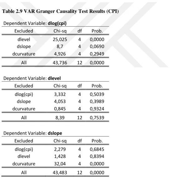
(CPI) ...63

T

ABLE

A.1

ENS

E

STIMATION

R

ESULTS OF

GRG

N

ON

L

INEAR

M

ETHODOLOGY

...76

T

ABLE

B.1

DNS

E

STIMATION

R

ESULTS OF

GRG

N

ON

L

INEAR

M

ETHODOLOGY

...84

T

ABLE

C.1

ENS

E

STIMATION

R

ESULTS OF

M

ATLAB

O

PT

.

M

ETHODOLOGY

...93

T

ABLE

D.1

DNS

E

STIMATION

R

ESULTS OF

M

ATLAB

O

PT

.

M

ETHODOLOGY

... 101

T

ABLE

E.1

DNS

E

STIMATION

R

ESULTS OF

OLS

M

ETHODOLOGY

... 109

T

ABLE

E.2

A

DJUSTED

R

V

ALUES AND

S

IGNIFICANCE OF

B

ETAS IN

OLS

M

ETHODOLOGY

... 117

T

ABLE

F.1

ENS

E

STIMATION

R

ESULTS OF

OLS

M

ETHODOLOGY

... 126

T

ABLE

F.2

T

URKISH

Y

IELD

C

URVES

E

STIMATED VIA

OLS

M

ETHODOLOGY

... 134

T

ABLE

G.1

G

RAPHICAL

R

EPRESENTATION OF

S

EASONALLY

A

DJUSTED

D

EPENDENT

V

ARIABLES

... 135

T

ABLE

G.2

G

RAPHS OF

D

EPENDENT

V

ARIABLES

’

L

OGARITHM

F

ORMS

... 137

T

ABLE

G.3

U

NIT

R

OOT

T

EST

R

ESULTS

... 139

T

ABLE

H.1

V

ARIABLE

D

ESCRIPTIONS OF

M

ODEL

2.3.1 ... 160

T

ABLE

H.2

V

ARIABLE

D

ESCRIPTIONS OF

M

ODEL

2.3.2 ... 160

T

ABLE

H.3

V

ARIABLE

D

ESCRIPTIONS OF

M

ODEL

2.3.3 ... 161

T

ABLE

I.1

E

CONOMETRIC

A

NALYSIS

R

ESULTS OF

M

ODEL

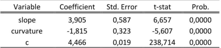
2.3.1... 162

T

ABLE

I.2

E

CONOMETRIC

A

NALYSIS

R

ESULTS OF

M

ODEL

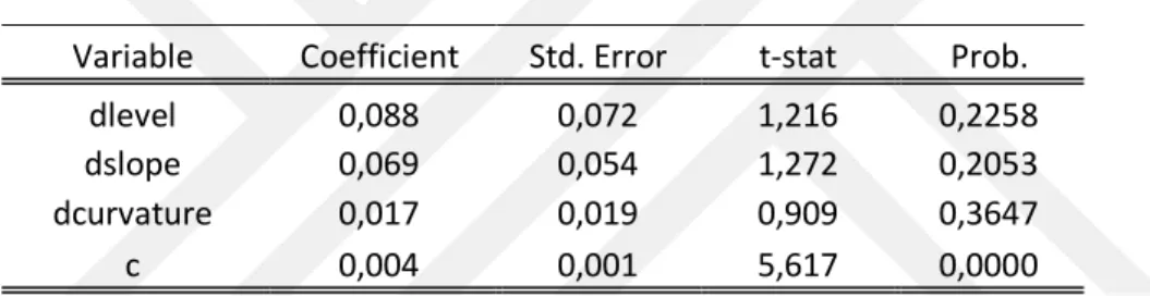
2.3.2... 163

T

ABLE

I.3

E

CONOMETRIC

A

NALYSIS

R

ESULTS OF

M

ODEL

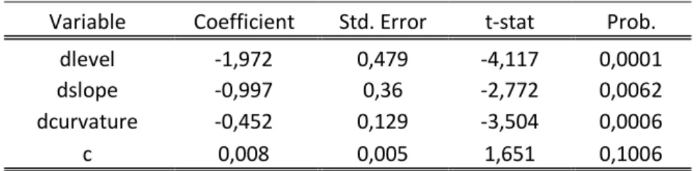
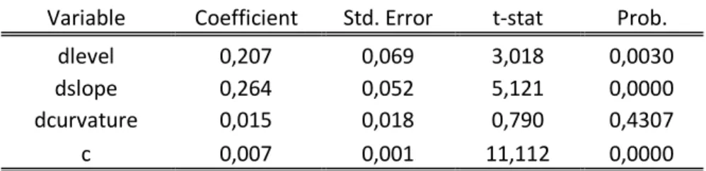
2.3.3... 167

(Note: Table 1.1 indicates the first table in Chapter 1, Table 2.1 indicates the first table in

Chapter 2 and Table A.1 indicates the first table in Appendix.)

vii

LIST OF GRAPHS

G

RAPH

‎1.1

E

STIMATED

T

URKEY

Y

IELD

C

URVES VIA

ENS

AND

DNS

FOR

2018

Q1 ...21

G

RAPH

‎1.2

C

OMPARISON OF

E

STIMATED

(GRG

N

ONLINEAR

)

AND

A

CTUAL

Y

IELDS

...22

G

RAPH

‎1.3

T

URKISH

Y

IELD

C

URVES

E

STIMATED VIA

ENS/DNS

GRG

N

ONLINEAR

...23

G

RAPH

‎1.4

C

OMPARISON OF

E

STIMATED

(M

ATLAB

)

AND

A

CTUAL

Y

IELDS

...25

G

RAPH

‎1.5

T

URKISH

Y

IELD

C

URVES

E

STIMATED VIA

ENS/DNS

M

ATLAB

O

PTIMIZATION

...26

G

RAPH

‎1.6

C

OMPARISON OF

E

STIMATED

(OLS)

AND

A

CTUAL

Y

IELDS

...28

G

RAPH

‎1.7

T

URKISH

Y

IELD

C

URVES

E

STIMATED VIA

OLS

M

ETHODOLOGY

...29

G

RAPH

‎1.8

C

OMPARISON OF

E

STIMATED

Y

IELDS

B

ASED ON

M

ATURITIES

...32

G

RAPH

2.1

T

IME

S

ERIES OF

E

STIMATED

DNS

P

ARAMETERS

...45

G

RAPH

2.2

T

IME

S

ERIES OF

D

EPENDENT

V

ARIABLES

...48

G

RAPH

2.3

US/UK

T

ERM

S

PREAD AND

R

ECESSIONS

...54

G

RAPH

2.4

T

URKEY

T

ERM

S

PREAD AND

R

ECESSIONS

...55

G

RAPH

2.5

T

URKEY

T

ERM

S

PREAD AND

B

EAR

M

ARKETS

...57

(Note: Graph 1.1 indicates the first graph in Chapter 1 and Graph 2.1 indicates the first graph in

Chapter 2.)

viii

ABBREVIATIONS

BIST100

: Istanbul Stock Exchange 100

CPI

: Consumer Price Index

DNS

: Dynamic Nelson-Siegel

ENS

: Extended Nelson-Siegel

EU

: European Union

GDP

: Gross Domestic Product

IPI

: Industrial Production Index

OLS

: Ordinary Least Squares

UK

: United Kingdom

ix

ABSTRACT

TEMUÇİN, TEOMAN SAMET. ESTIMATE THE YIELD CURVE FOR SOVEREIGN

BONDS IN TURKEY AND FORECASTING TURKISH ECONOMY FROM THE SHAPE

OF YIELD CURVE (2005 - 2018), Ph.D. THESIS, ISTANBUL, 2019

Yield curve that reflects the interest expectations of market participants is one of the

cornerstones of the financial analysis. In the first chapter of our study, Turkey yield

curve for sovereign bond market is estimated in 2005-2018 by using Extended

Nelson-Siegel (ENS) and Dynamic Nelson-Nelson-Siegel (DNS) models. Since Turkish sovereign

market becomes more liquid and 10-year fixed rate coupon bonds were started to be

traded after 2010, this allows us to make estimation for 10-year term to maturity. As a

result of estimation via two methodologies, it is concluded that Dynamic Nelson-Siegel

model estimates Turkey yield curve slightly better than the Extended Nelson-Siegel

model. Besides, OLS (Ordinary Least Square) is better methodology than optimization

tools in DNS.

This is why, the estimated Turkey yield curve via Dynamic Nelson-Siegel model with

OLS methodology is used to forecast Turkish macroeconomic and financial indicators

in the second chapter of the study. The yield curve can be simply perceived as a

representation of interest rates of treasury bonds or other security instruments in

different maturities. However, that simple graph is beyond the representation of interest

rate. If it is read carefully, the market efficiency theory can be beaten and regular profits

from the market can be made. Many scholars and empirical studies of them have proved

the significant forecasting ability of the yield curve about recessions, turning points in

the stock market and inflation rates. Therefore, it seems as a reliable mechanism for

forecasting to some important indicators in the macroeconomic set. I also simply test the

forecasting capabilities of the estimated Turkey yield curve on Turkish recessions, bear

market, industrial production index, bist100 index and consumer price index. As a result

of analysis, it is concluded that parameters, which represent the Turkey’s yield curve,

contain important information and predictions regarding recessions, bear market

formation, bist100 index and consumer price index.

x

Keywords: Sovereign Bonds, Yield Curve Estimation, Nelson Siegel, Turkey Yield

Curve, Forecasting Recession, Bear Market and Inflation

xi

ÖZET

TEMUÇİN, TEOMAN SAMET. TÜRKİYE HAZİNE KAĞITLARININ VERİM

EĞRİSİNİ TAHMİN ETMEK VE TÜRKİYE EKONOMİSİNİ VERİM EĞRİSİ

ÜZERİNDEN ÖNGÖRMEK (2005 - 2018), DOKTORA TEZİ, İSTANBUL, 2019

Piyasa katılımcılarının faiz beklentilerini yansıtan verim eğrileri finansal analizin temel

taşlarından biridir. Tezin 1.Bölümü’nde, 2005-2018 yılları arasındaki Türkiye Hazine

kağıtlarının verim eğrileri Extended Nelson-Siegel (ENS) ve Dynamic Nelson-Siegel

(DNS) modelleri aracılığıyla tahmin edilmiştir. 2010 yılından sonra Türkiye menkul

kıymet piyasalarının daha likit olması ve 10 yıllık Hazine kağıtlarının işlem görmeye

başlaması, verim eğrisi tahminlerimizin 10 yıllık yapılmasına imkan tanımıştır. İki

metodoloji ile yaptığımız verim eğrisi tahminleri üzerinden ulaşılan sonuç: Dynamic

Nelson-Siegel modelinin Türkiye verim eğrilerini Extended Nelson-Siegel modelinden

bir miktar daha iyi tahmin ettiği yönündedir. DNS modeli içerisinde ise, OLS

yönteminin optimizasyon araçlarına göre daha iyi bir yöntem olduğu sonucuna

ulaşılmıştır.

Araştırmamızın 2.Bölümü’nde, Dynamic Nelson-Siegel modeli OLS yöntemiyle elde

edilen verim eğrileriyle, Türkiye makroekonomik ve finansal verileri tahmin edilmeye

çalışılmıştır. Verim eğrisi, farklı vadelerde hazine bonosu ya da diğer menkul

kıymetlerin faizlerini gösteren basit bir eğri olarak algılanabilir ancak söz konusu eğri,

faizlerin temsilinden çok daha öte bir anlam taşımaktadır. Verim eğrisi dikkatli

okunursa, piyasa etkinliği teorisi kırılabilir ve hatta piyasadan düzenli kârlar elde

edilebilir. Birçok akademisyen ve bilimsel araştırma, verim eğrisinin resesyonları,

borsadaki dönüş anlarını ve enflasyon oranlarını tahmin etmede anlamlı sonuçlar

verdiğini kanıtlanmıştır. Bu yüzden verim eğrisi, makroekonomik kümedeki bazı

göstergeleri tahmin etmek için güvenilir bir araç olarak gözükmektedir. Çalışmanın

2.bölümünde, ilk bölümde tahmin ettiğimiz Türkiye verim eğrisinin; Türkiye’deki

resesyonları, ayı piyasasını, sanayi üretim endeksini, bist100 endeksini ve enflasyon

oranlarını öngörebilme kabiliyeti test edilmiştir. Analizlerin sonucunda, Türkiye verim

eğrisini temsil eden parametrelerin, Türkiye’de resesyon, ayı piyasası oluşumu, bist100

endeksi ve tüketici fiyat endeksinin gelişimine ilişkin önemli bilgi ve öngörüler içerdiği

tespit edilmiştir.

xii

Anahtar Sözcükler: Devlet Tahvili, Verim Eğrisi Tahmini, Nelson Siegel, Türkiye

Verim Eğrisi, Resesyon, Ayı Piyasası ve Enflasyon Tahmini

13

CHAPTER - 1

1.

ESTIMATING TURKEY YIELD CURVE FOR SOVEREIGN BONDS

1.1 INTRODUCTION

Yield curve (also known as term structure of interest rates or spot rate curve) indicates

the relationship between interest rate of security and term to maturity. The main benefit

of estimating yield curve is that having interest rate data without being affected by

interest rate fluctuation of specific bonds (Akıncı et al., 2006). Besides, estimating

accurate yield curve is crucial for monetary policy decisions and portfolio management.

If discounted bonds that have term to maturity from one-day to ten-year and traded on a

daily basis, then the graph of these bonds’ interest rate would automatically give the

yield curve. However, since we have a limited number of securities with specific term to

maturity, we need to estimate yield curve.

There are several methodologies which estimate the yield curve in literature. Bliss and

Fama (1987) got available spot rate and then estimated the curve via regression. This

method is called as smoothed bootstrap (Annaert et al., 2012). Similar to this method,

there are other curve fitting spline methods that include many estimated parameters such

as quadratic and cubic splines (McCulloch (1971, 1975)), exponential splines (Vasicek

and Fong, 1982), basis splines (Steeley, 1991), maximum smoothness splines (Adams

and Deventer, 1994) and roughness penalty function splines (Fisher et al., 1994;

Waggoner, 1997).

Under the models of the short rate, some apply equilibrium method which models the

dynamics of the instantaneous rate and obtains yields at other maturities under specific

assumptions about risk premium. Vasicek (1977), Cox et al. (1985) and Duffie and Kan

(1996) are important contributors to equilibrium methodology. Some use no-arbitrage

method which tries to fit the yield curve at a point in which there is no chance of

14

arbitrage. We mean that the yield curve is estimated by eliminating the possibility of

arbitrage returns with different maturities. Hull and White (1990) estimated yield curve

by comparing the results of two models and interest rate option prices. Brennan and

Schwartz (1979) and Ho and Lee (1986) are other contributors to the no-arbitrage

methodology. Unlike these academics in no-arbitrage literature, Heath-Jarrow-Morton

(1992) differently modeled the entire forward curve as opposed to simple short rate.

Models mentioned so far are mainly used for derivative pricing. Lastly and popularly,

parametric models are used for estimating yield curve. In this group, Nelson-Siegel

(1987) model, its extension by Svensson (1994) and its dynamic version by Diebold and

Li (2006) are widely used by central banks, academia and other market participants for

estimating yield curve. Nelson-Siegel built a static model which makes a curve fitting of

the current data regardless of forward time period. The logic of these models will be

explained in the next section.

The purpose of this chapter of the thesis is to estimate Turkey yield curve for discounted

and fixed coupon government bonds by applying the Nelson‐Siegel model’s derivatives,

namely Extended Nelson-Siegel (ENS) and Dynamic Nelson-Siegel (DNS) models.

Since these methods are commonly used by many financial institutions and there is a

consensus in literature on their quality for fitting better yield curves, we apply ENS and

DNS for estimating Turkey yield curve. As a result of estimation, although both ENS

and DNS have very similar shapes for yield curve, DNS estimates Turkey yield curve

slightly better than ENS by comparing their sum of squares of deviation between

theoretical price and dirty price of securities. Besides, OLS technique in DNS

methodology performs better in estimating yield curves than optimization techniques.

The figures regarding these figures will be shared in the following sections.

First chapter of the thesis is organized as follows. In section 1.2, a detailed explanation

and formulas of Nelson-Siegel model and its derivatives will be discussed. Besides, we

provide how they interact and contribute to each other to estimate yield curve. In section

1.3, our data for Turkish sovereign bond market and methodologies for estimating will

be introduced. In section 1.4, estimated yield curve, founded ENS and DNS parameters

15

and their advantages and disadvantages will be evaluated and compared. In the final

section, our concluding remarks regarding Chapter-1 of the thesis will be mentioned.

1.2 EXTENDED AND DYNAMIC NELSON-SIEGEL MODELS

Nelson and Siegel (1987) estimated the yield curve by using four parameters. (1.2.1)

According to the authors, β

0

, β

1

and β

2

represent the short, medium and long-term

components of the yield curve. The long term component is represented via β

0

because

it remains constant when term to maturity parameter (T) evolves. β

1

serves the

representation of short-term and β

2

contributes the representation of the medium-term

component. As Ibanez (2016) stated, the fourth parameter (𝜆), which is not entirely

described, is a decay factor. That’s means it influences the fitting power of the model.

r(T) = β

0

+ (β

1

+ β

2

)

1 − e

−

𝑇

𝜆

𝑇

𝜆

– β

2

𝑒

−

𝑇

𝜆

_(1.2.1)

where β

0

, β

1

, β

2

and

𝜆 are parameters (𝜆 must be positive) to be extracted from the

current bond price.

The Extended Nelson Siegel (ENS) Model Svensson (1994) added an extension to the

model in order to fit better and capture highly non-linear, in other words hump-shape

(or U-shape), yield curves. Therefore, the curve is estimated by using six parameters.

(1.2.2) The logic of estimation is the same as in the case of the Nelson Siegel model.

r(T) = β

0

+ (β

1

+ β

2

)

1 − e

−

𝑇

𝜆1

𝑇

𝜆1

– β

2

𝑒

−

𝑇

𝜆1

_{+ β}

₃

(

1 − e

−

𝑇

𝜆2

𝑇

𝜆2

− e

−

𝜆2

𝑇

)

_(1.2.2)

where β

0

, β

1

, β

2

, β

3

, 𝜆

1

and 𝜆

2

are parameters (𝜆

1

and 𝜆

2

must be positive) to be extracted

from the current bond price.

The Dynamic Nelson Siegel (DNS) Model Diebold and Li (2006) introduced the

dynamic version of the Nelson Siegel model. (1.2.3) The most important contribution of

them to the literature, DNS parameters that represent the curve can be used for

forecasting purposes as well. In other words, they reinterpreted the parameters as level

16

factor therefore it is β

1

= yt(∞). The slope parameter (β

2

) represents the short-term

factor which is defined as ten-year yield minus the three-month yield by Diebold and Li,

i.e. β

2

= y

t

(120) – y

t

(3). The curvature parameter (β

3

) represents the medium-term factor

which is defined as twice the two-year yield minus the sum of the ten-year and

three-month yields, i.e. β

3

= 2y

t

(24) - (y

t

(120) + y

t

(3)). Later on, we will also graph estimated

parameters against β

1

, β

2

, β

3

and test whether the logic works for Turkey as well or not

in Chapter-2. Although 4 parameters could be estimated by nonlinear least squares,

Diebold and Lie preferred to fix

𝜆 at a predefined value so as to increase reliability of

betas. Now, betas could be estimated by using ordinary least squares because

non-linearity in the equation is eliminated by fixing 𝜆.

r(T) = β

1

+ β

2

(

1 − e

−λT

λT

) + β

3

(

1 − e

−λT

λT

− e

−λT

₎

_(1.2.3)

where β

1

, β

2

, β

3

and

𝜆 are parameters (𝜆 must be positive) to be extracted from the

current bond price.

In the following sections, we will estimate Turkey’s yield curve for sovereign bond

market by using these two methodologies, namely ENS and DNS. ENS will be applied

in order to achieve a better fit yield curve because it contains hump-shape as well by

using six parameters. DNS will be also applied so as to get foreseeable parameters and

use them for forecasting purposes in Chapter-2 of the thesis.

17

1.3 DATA AND METHODOLOGY

The data consists of monthly observations of Turkish sovereign bonds and bills market

in the period of February 2005-December 2018. One of the most important feature of

our thesis is that Turkish yield curve would be estimated with the latest bond market

data. We need to point out that Turkish sovereign market becomes more liquid and

longer maturities are started to be traded in the same period as well. This is why it is

necessary to make such a kind of work for current data in order to get longer and

trustworthy yield curves. February 2005 is chosen as a starting point because 5-year

fixed coupon rate bonds were started to be traded in Turkey. Besides, Turkish financial

markets became more transparent, accountable and officially controlled in early 2000s

with the foundation of new financial regulatory bodies such as Banking Regulation and

Supervision Agency and additional precautions were taken in order to protect investors.

On the other hand, 10-year fixed coupon rate bonds were started to be traded in January

2010. We conclude that estimating 10-year yield curve without having a security with

10-year term to maturity and traded in the market would give incorrect estimation

results. This is why although yield curves which have 5-year term to maturity are

estimated in 2005-2010, 10-year yield curves are estimated for 2010-2018 period.

The data is received from Istanbul Stock Exchange database. Each day’s data reports

value date, days to maturity, days to coupon, accrued interest, prices, simple and

compound rate of return and transaction volume of each security. Since the data is daily,

the last business day of each month is used as a representative of the related month. The

sample consists of 167 months (n=167). Although both fixed coupon and floating rate

bonds are issued in the period, we only apply TL denominated zero-coupon and

fixed-coupon rate bonds for curve estimation since cash flows of floating rate bonds cannot be

determined in advance.

Besides, the 7-9 most liquid sovereign bonds of each specific day to maturity (around

3-month, 6-3-month, 1-year, 2-year, 3-year, 4-year, 5-year, 7-year and 10-year) are chosen

for estimating yield curve. For instance, if the last business day of the month includes

15 sovereign bonds, we choose the most liquid 9 of them which represent specific days

to maturity and exclude illiquid ones by working in each 167 of them manually. The

18

reason why we do this is that the price of illiquid ones could manipulate the estimation

results and estimated yield curves will not reflect the reality. Besides thanks to this

method, the possibility of manipulating the entire data of the securities that are focused

on a certain period (such as from 1 month to the 1 year) has been eliminated. Moreover,

since Istanbul Stock Exchange’s daily data does not include coupon rates of the bonds,

we calculated them by using accrued interest. The coupon rates are calculated with the

following formula

1

;

C = (

364 × AI

182−Days to Coupon

)

(1.3.1)

where C represents coupon rate and AI represents accrued interest.

Weighted average price is used as clean price and dirty price is calculated by summing

up clean price and accrued interest of each bond. After we calculate r(T) by using

formula (1.2.2) and (1.2.3), present value of each coupon and principal payments are

obtained. We reach ENS and DNS theoretical prices by summing up all present values

of coupon and principal payments. And then, we minimize the sum of the squared

deviations of the dirty prices from the estimated theoretical prices of 9 bonds found via

ENS and DNS. (1.3.2)

min. A(β

0

, β

1

, β

2

, β

3

, 𝜆

1

, 𝜆

2

) = ∑

(𝑃

_𝑖

𝐸𝑁𝑆/𝐷𝑁𝑆

− 𝑃

_𝑖

𝐷𝑖𝑟𝑡𝑦 (𝐷𝑎𝑡𝑎)

)

2

9

𝑛=1

(1.3.2)

We apply two methodologies, namely GRG nonlinear and Matlab optimization tools in

order to minimize the sum of the squared deviations between dirty price and ENS/DNS

theoretical prices.

Besides, we apply ordinary least squares as a different technique for estimating

Turkey’s yield curve. Diebold and Li (2006) defined 𝜆 as if it determines the maturity at

which the loading on the curvature factor (β

3

) reaches its maximum and fixed

𝜆 at a

predefined value by assuming 30 months used as medium term in US sovereign bond

market. Since Diebold and Li worked on a developed economy, we need to fix

𝜆 at a

1

19

different value so as to reflect Turkey yield curve accurately. Murat Duran (2014) fixed

𝜆 at 1,017 for Turkey yield curve estimation between 2010 and 2014. We realize that

the loading on the medium-term (curvature) factor, i.e. ((1 − e

−λT

_{)/λT) − e}

−λT

_{, is}

maximized at around 24 months (T=2) for Turkey case. Therefore, the curvature factor

(β

3

) reaches its maximum at 𝜆=0,897 by assuming 24 months (T=2) as medium term in

Turkish sovereign bond market in order to use ordinary least squares for estimating

betas. After all, we fix 𝜆 at 0,897 for the period of February 2005-December 2018 when

we apply OLS methodology of Diebold&Li for estimating betas.

Moreover, we attempt to add a new perspective to the literature. We simply apply

Diebold&Li’s technique of OLS beta estimation for Svensson (ENS) formula as well.

After making some mathematical adjustments on Svensson formula (1.2.2), we get

(1.3.3) for Extended Nelson Siegel Model. This mathematical representation of ENS

formula also exists in Gilli et al.’s (2010) working paper:

r(T) = β

0

+ β

1

(

1 − e

−

𝑇

𝜆1

𝑇

𝜆1

) + β

2

(

1 − e

−

𝑇

𝜆1

𝑇

𝜆1

− e

−

𝑇

𝜆1

) + β

₃

(

1 − e

−

_𝜆2

𝑇

𝑇

𝜆2

− e

−

𝑇

𝜆2

) (1.3.3)

Now, we adapt Diebold&Li’s curvature interpretation to Svensson model and the

loading on the medium-term (curvature) factors are maximized at

𝜆

1

=1,115 and

𝜆

2

=2,788 by assuming 24 months (T=2) as first curvature and 60 months (T=5) as

second curvature (medium term) of the yield curve respectively in Turkish sovereign

bond market. After fixing 𝜆

1

at 1,115 and 𝜆

2

at 2,788, we apply ordinary least squares

for estimating 4 betas in 1.3.3 as a new attempt.

However, we do not fix any

𝜆 value during GRG nonlinear or Matlab optimization

techniques of ENS/DNS estimations. Since we decide to use the optimization method in

order to minimize the sum of the squared deviations (1.3.2), adding an extra constraint

to the equations makes the estimation results inefficient. This is why we do not fix any

parameter at all during the optimization techniques.

20

1.4 ESTIMATION RESULTS AND COMPARISON OF METHODS

1.4.1. GRG Nonlinear Optimization Method

Both ENS and DNS model do not work perfectly because running a standard

optimization technique could not achieve complete price equality between theoretical

and realized dirty prices for 167 observations. However, the difference is minor for

most of our data. The sum of the squared deviations between ENS theoretical price and

dirty price for bonds is less than “2” for 94% of our daily observations. The same ratio

is %96 for DNS. We can also conclude that DNS estimates Turkey yield curve slightly

better than ENS model by comparing their sum of square deviations between theoretical

prices and dirty prices of securities. Although the sum of square deviation is 129,2 in

ENS methodology for 167 observations, the sum is 101,3 for DNS methodology.

As mentioned above, we work on last business day of every month one by one and

apply optimization method GRG nonlinear in Excel. Let us discuss first quarter of 2018

ENS and DNS results as an example for closer inspection by comparing their

theoretical/dirty prices, sum of squared errors and shape of yield curves (Table 1.1,

Table 1.2 and Graph 1.1) before presenting whole results for 167 observations.

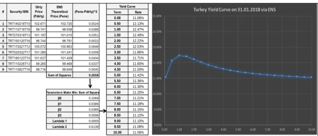
Table 1.1 Example: How to Estimate Turkey Yield Curve via ENS on 31.01.2018

Table-1.1. shows how Turkey yield curve on 31.01.2018 is calculated via ENS. First, dirty prices of the most liquid 9 securities

based on specific day to maturity are got from Istanbul Stock Exchange database and they are compared with calculated ENS

theoretical prices. The optimal ENS parameters are determined by minimizing the sum of difference between dirty and ENS

theoretical prices based on GRG nonlinear. Then, Turkey yield curve is plotted with optimal ENS parameters based on different

terms.

Term Rate 0.08 11.06% 1 TRT140218T10 102.671 102.720 0.0024 0.50 12.13% 2 TRT110718T18 98.741 98.938 0.0388 1.00 12.47% 3 TRT270319T13 101.197 101.010 0.0351 1.50 12.40% 4 TRT150120T16 96.744 96.791 0.0022 2.00 12.22% 5 TRT170221T12 100.572 100.863 0.0848 2.50 12.03% 6 TRT020322T17 101.385 101.241 0.0208 3.00 11.86% 7 TRT180123T10 101.637 101.429 0.0434 3.50 11.71% 8 TRT110226T13 99.285 99.468 0.0337 4.00 11.60% 9 TRT110827T16 98.716 98.649 0.0045 4.50 11.50% Sum of Squares 0.2658 5.00 11.42% 5.50 11.36% 6.00 11.30% 6.50 11.25% β0 0.1069 7.00 11.21% β1 0.0386 7.50 11.18% β2 0.0386 8.00 11.15% β3 0.0596 8.50 11.12% Lambda 1 0.0000 9.00 11.10% Lambda 2 0.6138 9.50 11.08% 10.00 11.06% Parameters Make Min. Sum of Square

Yield Curve # Security ISIN Dirty Price (Pdirty) ENS Theoretical Price (Pens) (Pens-Pdirty)^2 8.00% 9.00% 10.00% 11.00% 12.00% 13.00% 14.00% 15.00% 0.00 1.00 2.00 3.00 4.00 5.00 6.00 7.00 8.00 9.00 10.00

21

Table 1.2 Comparison of Optimal Parameters of ENS and DNS for 2018 Q1

Date

Parameters that Make Min. Sum Of Squares via ENS

Parameters that Make Min. Sum Of Squares via DNS

Beta 0

Beta 1

Beta 2

Beta 3

Alfa 1

Alfa 2

(Zthe-Zreal)^2 Beta 1

Beta 2

Beta 3

Alfa 1

(Ztheo-Zdirty)^2

31.01.2018

0.1069

0.0386

0.0386

0.0596

0.0000

0.6138

0.27

0.1067

0.0087

0.0455

1.4339

0.25

28.02.2018

0.1056

0.0386

0.0386

0.0611

0.0000

0.7719

0.73

0.1049

0.0155

0.0358

0.9770

0.61

30.03.2018

0.1065

0.0386

0.0386

0.0936

0.0000

0.8298

1.46

0.1059

0.0108

0.0762

1.0585

1.39

Table-1.2. shows ENS/DNS optimal parameters and the sum of difference between dirty and ENS/DNS theoretical prices based on

GRG nonlinear for 2018 Q1.

Graph 1.1 Estimated Turkey Yield Curves via ENS and DNS for 2018 Q1

Graph-1.1. illustrates Turkey yield curve for 2018 Q1 with optimal ENS and DNS parameters based on different terms (years).

Before we present entire ENS and DNS yield curves for the period of 2005-2018 via

GRG Nonlinear, let us lastly compare the estimated yields and actual data for selected

31.01.2018

28.02.2018

30.03.2018

8,0%

9,0%

10,0%

11,0%

12,0%

13,0%

14,0%

15,0%

0

₁

2

₃

4

₅

6

₇

8

₉

10

Sp

o

t

R

at

e

Term (Years)

ENS

31.01.2018

28.02.2018

30.03.2018

8,0%

9,0%

10,0%

11,0%

12,0%

13,0%

14,0%

15,0%

0

₁

2

₃

4

₅

6

₇

8

₉

10

Sp

o

t

R

at

e

Term (Years)

DNS

22

dates. We use weighted average simple rate of return from Istanbul Stock Exchange

database as actual data. The estimated yields are randomly selected based on their

representation of different kind of shapes. I mean that although most of the Turkey’s

yields have increasing function, we chose decreasing and constant yields as well.

According to the results, both ENS and DNS are capable of representing different

shapes of yield curves. However, it is worth mentioning an important point here that

both yields estimated via ENS and DNS using optimization GRG nonlinear technique

underestimate the actual values. This is important because this graphical representation

clearly proves the poor performance of estimations. Secondly, ENS is more successful

especially for humped shapes (such as 30.03.2012) as it is expected because ENS model

has an extension in order to fit better and capture highly non-linear, in other words

hump-shape, yield curves as well. (Graph 1.2)

Graph 1.2 Comparison of Estimated (GRG Nonlinear) and Actual Yields

Graph 1.2. illustrates actual (data-based) and fitted (ENS/DNS model-based) Turkey yield curves for selected dates.

Finally, we follow the same methodology for all data, obtain time series of optimal

ENS/DNS parameters and estimate Turkey yield curve for 167 observations via both

6,00%

7,00%

8,00%

9,00%

10,00%

11,00%

0,00

2,00

4,00

6,00

8,00

10,00

Yield Curve on 29.01.2010

ENS

Actual

DNS

8,50%

9,00%

9,50%

10,00%

0,00

2,00

4,00

6,00

8,00

10,00

Yield Curve on 30.03.2012

ENS

Actual

DNS

8,50%

9,50%

10,50%

11,50%

0,00

2,00

4,00

6,00

8,00

10,00

Yield Curve on 31.08.2015

ENS

Actual

DNS

14,00%

15,00%

16,00%

17,00%

18,00%

19,00%

20,00%

21,00%

0,00

2,00

4,00

6,00

8,00

10,00

Yield Curve on 30.11.2018

ENS

Actual

DNS

23

methodologies. (See all estimated results in Appendix A and B) Although there is a

little difference between the sum of squared errors of both methods and DNS is slightly

better for estimating Turkey’s yield curve, the graphical representation of the estimation

for two methodologies as a whole is mainly similar to each other. (Graph 1.3)

Graph 1.

3

Turkish Yield Curves Estimated via ENS/DNS GRG Nonlinear

28.02.2005

28.02.2006

28.02.2007

29.02.2008

27.02.2009

26.02.2010

28.02.2011

29.02.2012

28.02.2013

28.02.2014

27.02.2015

29.02.2016

28.02.2017

28.02.2018

0%

5%

10%

15%

20%

25%

30%

0

,0

8

₂

4

₆

8

10

Sp

o

t

R

at

e

(%

)

Term

Turkish Yield Curves via ENS

28.02.2005

28.02.2006

28.02.2007

29.02.2008

27.02.2009

26.02.2010

28.02.2011

29.02.2012

28.02.2013

28.02.2014

27.02.2015

29.02.2016

28.02.2017

28.02.2018

0%

5%

10%

15%

20%

25%

30%

0

,0

8

₂

4

₆

8

10

Sp

o

t

R

at

e

(%

)

Term (Years)

24

Graph 1.3 plots Turkey yield curves between 2005.02 and 2018.12 via ENS and DNS methodology via GRG Nonlinear. The sample

consists of 167 observations. Since 10-year fixed coupon rate bonds were started to be traded after January 2010, estimated yield

curves which have 5-year term to maturity are plotted in 2005-2010. And, 10-year yield curves (term to maturity) are plotted for

2010-2018 period.

1.4.2. Matlab Optimization Method

What we did in Excel’s GRG Nonlinear optimization tool in 1.4.1. is repeated in this

section by using another software program, namely Matlab optimization tool. We apply

Matlab’s fmincon function which finds minimum of constrained nonlinear multivariable

functions for optimization. The purpose of repeating the same process in another

program is that the Matlab’s optimization might perform better estimations by reducing

the difference to a smaller value between theoretical and dirty prices. In other words, we

expect to solve the underestimation problem of GRG Nonlinear via Matlab’s fmincon

function. However comparing to GRG Nonlinear’s results, Matlab’s optimization tool

performs worse. In Matlab’s results, the sum of the squared deviations between ENS

theoretical price and dirty price for bonds is less than “2” for only 40% of our

observations. The ratio is %41 for DNS. We can also conclude that DNS estimates

Turkey yield curve slightly better than ENS model in Matlab too by comparing their

sum of square deviations between theoretical prices and dirty prices of securities.

Although the sum of square deviation is 1.455,9 in ENS methodology for 167

observations, the sum is 1.447,8 for DNS methodology. However, these results are very

high in compare to GRG Nonlinear optimization results, this is why we can conclude

that GRG Nonlinear performs better for estimating Turkey’s yield curve than Matlab’s

fmincon function.

Let us compare the estimated yields of Matlab and actual data for selected dates too. We

use weighted average simple rate of return from Istanbul Stock Exchange database as

actual data. The same yields are selected based on their representation of different kind

of shapes parallel to section 1.4.1. (Graph 1.4)

25

Graph 1.

4

Comparison of Estimated (Matlab) and Actual Yields

Graph 1.4. illustrates actual (data-based) and fitted (ENS/DNS model-based) Turkey yield curves for selected dates via Matlab

optimization

Lastly, we estimate Turkey yield curve for 167 observations via Matlab’s fmincon

optimization tool for both ENS and DNS. (See fmincon optimization code details and

all estimated results in Appendix C and D) Let us look at the graphical representation

of the estimated yield curves. (Graph 1.5)

6,00%

7,00%

8,00%

9,00%

10,00%

11,00%

0,00

2,00

4,00

6,00

8,00

10,00

Yield Curve on 29.01.2010

ENS

Actual

DNS

8,50%

9,00%

9,50%

10,00%

0,00

2,00

4,00

6,00

8,00

10,00

Yield Curve on 30.03.2012

ENS

Actual

DNS

8,50%

9,50%

10,50%

11,50%

0,00

2,00

4,00

6,00

8,00

10,00

Yield Curve on 31.08.2015

ENS

Actual

DNS

14,00%

15,00%

16,00%

17,00%

18,00%

19,00%

20,00%

21,00%

0,00

2,00

4,00

6,00

8,00

10,00

Yield Curve on 30.11.2018

ENS

Actual

DNS

26

Graph 1.

5

Turkish Yield Curves Estimated via ENS/DNS Matlab Optimization

Graph 1.5 plots Turkey yield curves between 2005.02 and 2018.12 by ENS and DNS methodology via Matlab optimization. The

sample consists of 167 observations. Since 10-year fixed coupon rate bonds were started to be traded after January 2010, estimated

28.02.2005

28.02.2006

28.02.2007

29.02.2008

27.02.2009

26.02.2010

28.02.2011

29.02.2012

28.02.2013

28.02.2014

27.02.2015

29.02.2016

28.02.2017

28.02.2018

0%

5%

10%

15%

20%

25%

30%

35%

40%

0

,0

8

₂

4

₆

8

10

Sp

o

t

R

at

e

(%

)

Term

Turkish Yield Curves via ENS

28.02.2005

28.02.2006

28.02.2007

29.02.2008

27.02.2009

26.02.2010

28.02.2011

29.02.2012

28.02.2013

28.02.2014

27.02.2015

29.02.2016

28.02.2017

28.02.2018

0%

5%

10%

15%

20%

25%

30%

35%

0

,0

8

₂

4

₆

8

10

Sp

o

t

R

at

e

(%

)

Term (Years)

27

yield curves which have 5-year term to maturity are plotted in 2005-2010. And, 10-year yield curves (term to maturity) are plotted

for 2010-2018 period.

Not only Matlab has the problem of underestimating the yield curve similar to Excel

GRG Nonlinear methodology, but also Matlab has major deficiencies regarding

estimation. First of all, Matlab shows the rate of short-term sections of the curves (such

as 1-12 months) higher than expected. (Graph 1.5) Secondly, although most of the

yields should have a curvature shape or increasing/decreasing function at least, Matlab’s

fmincon function estimates a horizontal curve for most of the data, especially in

2010-2017.

1.4.3. Ordinary Least Squares Method

We have not obtained desired estimation results yet in both optimization methodologies,

therefore we apply a new one. Diebold&Li (2006) proposed a dynamic approach for

estimating yield curves such that they used interest rates and extracted beta values (β

1

,

β

2

and β

3

) by applying ordinary least squares regression analysis to the equation (1.2.3).

They fixed

𝜆 at a constant value such that betas could be estimated by using ordinary

least squares because non-linearity in the equation is eliminated by fixing 𝜆.

r(T) = β

1

+ β

2

(

1 − e

−λT

λT

) + β

3

(

1 − e

−λT

λT

− e

−λT

₎

_(1.2.3)

As we mention in section 1.3 of the thesis, we fix 𝜆 at 0.897 and make our consolidated

OLS regression analysis via Stata software.

All estimation results with adjusted R values and significance level of betas exist in

Appendix E. Briefly, most of the variables, especially all of the β

1

(level), are

statistically significant. Besides, adjusted R

2

are mainly above 90%.

Before sharing all estimation results, let us again compare the estimated yields and

actual data for selected dates. We use weighted average compound rate of return from

Istanbul Stock Exchange database as actual data. The same yields are selected based on

28

their representation of different kind of shapes parallel to methodologies in section 1.4.1

and 1.4.2. (Graph 1.6)

Graph 1

.6

Comparison of Estimated (OLS) and Actual Yields

Graph 1.6. illustrates actual (data-based) and fitted (DNS model-based) Turkey yield curves for selected dates via OLS.

It is clearly seen that the most accurate estimation results are got via OLS method for

selected four dates because estimated curves pass through the actual values, instead of

falling below them. Let us evaluate the graphical representation of 167 estimated yield

curves via OLS. (Graph 1.7)

7,00%

8,00%

9,00%

10,00%

11,00%

12,00%

0,00

2,00

4,00

6,00

8,00

10,00

Yield Curve on 29.01.2010

Actual

DNS

8,50%

9,00%

9,50%

10,00%

10,50%

0,00

2,00

4,00

6,00

8,00

10,00

Yield Curve on 30.03.2012

Actual

DNS

8,50%

9,50%

10,50%

11,50%

0,00

2,00

4,00

6,00

8,00

10,00

Yield Curve on 31.08.2015

Actual

DNS

16,00%

17,00%

18,00%

19,00%

20,00%

21,00%

22,00%

0,00

2,00

4,00

6,00

8,00

10,00

Yield Curve on 30.11.2018

Actual

DNS

29

Graph 1

.7

Turkish Yield Curves Estimated via OLS Methodology

Graph 1.7 plots Turkey yield curves between 2005.02 and 2018.12 via DNS methodology via OLS technique. The sample consists

of 167 observations. Since 10-year fixed coupon rate bonds were started to be traded after January 2010, estimated yield curves

which have 5-year term to maturity are plotted in 2005-2010. And, 10-year yield curves (term to maturity) are plotted for 2010-2018

period.

A New Attempt: Applying OLS Methodology for ENS

Since the estimated yield curves pass through actual rates for randomly selected four

days and we get reasonable 167 estimated yields that have no marginal trends or jumps,

we apply the Diebold&Li (2006) approach to the modified version of ENS formula

(1.3.3) as well. Honestly, we have not encountered this kind of study or attempt in

literature review such that trying to estimate four betas of Svensson by using OLS.

r(T) = β

0

+ β

1

(

1 − e

−

𝑇

𝜆1

𝑇

𝜆1

) + β

2

(

1 − e

−

𝑇

𝜆1

𝑇

𝜆1

− e

−

𝜆1

𝑇

) + β

₃

(

1 − e

−

_𝜆2

𝑇

𝑇

𝜆2

− e

−

𝜆2

𝑇

) (1.3.3)

Similar to Diebold&Li, we fix 𝜆

1

at 1,115 and

𝜆

2

at 2,788 which maximize the loading

factors of curvature terms for 24 and 60 months respectively and then try ordinary least

squares for estimating betas in 1.3.3. However, the results are not as we expected. We

28.02.2005

28.02.2006

28.02.2007

29.02.2008

27.02.2009

26.02.2010

28.02.2011

29.02.2012

28.02.2013

28.02.2014

27.02.2015

29.02.2016

28.02.2017

28.02.2018

0%

5%

10%

15%

20%

25%

30%

0

,0

8

₂

4

₆

8

10

Sp

o

t

R

at

e

(%

)

Term (Years)

30

could not succeed to get significant results and accurate estimations for Svensson

formula (ENS) as we did with Diebold&Li’s (DNS). The details of the estimation

results and graph of consolidated yield curves appear in Appendix F. In short, there are

even negative estimated yields that are impossible for Turkish economy. Besides, there

are very irrelevant results in 2005-2010 when we generally have 7 securities

(observations) in our regression analysis. That’s mean trying to estimate four variables

by using only 7 observations makes getting an accurate estimation result impossible. To

sum up, OLS method is used to estimate three independent variables (β

1

, β

2

and β

3

) in

Diebold&Li’s formula, is not successful in estimating four independent variables (β

0,

β

1

,

β

2

and β

3

) in Svensson’s formula. Therefore, our attempt to add a new perspective to the

31

1.4.4. Comparison of Methods

As it is remembered, sum of squared errors between theoretical and dirty prices are

higher in Matlab’s fmincon optimization tool. Graph 1.4 proves similar results such that

Matlab’s optimization tool is worse than Excel’s GRG Nonlinear optimization.

According to Graph 1.4, the Matlab tool does not only underestimate the yield curve,

but also follows irrelevant trends on the selected days. Therefore, we conclude that the

results are produced by the Excel GRG Nonlinear tool are more accurate than the results

of Matlab’s fmincon optimization tool.

By the way, minimizing the difference between theoretical price and dirty price via

optimization of GRG Nonlinear and Matlab fmincon optimization techniques do not

perfectly estimate the yield curves. Therefore, we could not find the desired betas which

equalize the difference to “0” between theoretical and dirty prices via optimization.

According to the literature, this problem stems from “local minima”. (Hladikova,

Radova (2012) and Gilli et. al. (2010)) It is basically argued that the optimization

methods can find local minima instead of global minima (i.e. equal to 0). Therefore, we

can estimate the yield curve, yet it is not an ideal one.

At the same time, when we evaluate the Graph 1.2 and 1.4, it is concluded that the

estimated yield curves obtained via two optimization methods are below the actual rates

and thus the yield curves are underestimated. Eventually, another method is needed in

order to achieve more accurate yields by eliminating the constraints and problems of

optimization methodologies: Ordinary Least Squares (OLS).

Eventually, we compare 3 methodologies, namely Excel GRG Nonlinear opt., Matlab

fmincon opt. and OLS, of estimated yields that are derived from DNS formula based on

their maturities (Graph 1.8). And, we conclude that OLS is the best methodology for

estimating yield curves.

- First of all, Matlab optimization is baddish especially in estimating shorter

maturities of yield curve as we discussed before. This is why blue line, that

represents Matlab, differentiates from OLS and GRG Nonlinear methods

32

especially in 1 month-1 year maturities of the curves. It overreacts and makes

unreasonable jumps. And, this unreasonable jumps also explain why Matlab

technique’s sum of square deviation between theoretical and dirty price is very

higher than the GRG Nonlinear technique.

- Secondly, although GRG Nonlinear estimates more accurate yield curves than

Matlab optimization technique, it is still unsuccessful in compare to OLS

methodology. It can easily seen that green line, that represents GRG Nonlinear

methodology, is generally under the red line, that represents OLS methodology,

in most of maturities. That’s mean GRG Nonlinear optimization technique

unfortunately underestimates the yield curves.

As a result of our tests, we conclude that OLS methodology is the best alternative

for estimating Turkish yield curve.

Graph 1

.8 Comparison of Estimated Yields Based on Maturities

Graph 1.8 plots comparison of three DNS estimated yields via GRG Nonlinear optimization (green

lines), Matlab’s fmincon

optimization (

blue

lines) and ordinary least squares (

red

lines) based on different maturities, such as 1 month, 3-6-12 months and

2-3-4-5-6-7-8-9-10 years.

0

0,05

0,1

0,15

0,2

0,25

28.02.2005 28.02.2006 28.02.2007 29.02.2008 28.02.2009 28.02.2010 28.02.2011 29.02.2012 28.02.2013 28.02.2014 28.02.2015 29.02.2016 28.02.2017 28.02.2018

Matlab DNS

OLS DNS

GRG DNS

1 Month

33

0

0,05

0,1

0,15

0,2

0,25

28.02.2005 28.02.2006 28.02.2007 29.02.2008 28.02.2009 28.02.2010 28.02.2011 29.02.2012 28.02.2013 28.02.2014 28.02.2015 29.02.2016 28.02.2017 28.02.2018

Matlab DNS

OLS DNS

GRG DNS

3 Months

0

0,05

0,1

0,15

0,2

0,25

28.02.2005 28.02.2006 28.02.2007 29.02.2008 28.02.2009 28.02.2010 28.02.2011 29.02.2012 28.02.2013 28.02.2014 28.02.2015 29.02.2016 28.02.2017 28.02.2018

Matlab DNS

OLS DNS

GRG DNS

6 Months

0

0,05

0,1

0,15

0,2

0,25

28.02.2005 28.02.2006 28.02.2007 29.02.2008 28.02.2009 28.02.2010 28.02.2011 29.02.2012 28.02.2013 28.02.2014 28.02.2015 29.02.2016 28.02.2017 28.02.2018

Matlab DNS

OLS DNS

GRG DNS

1 Year

34

0

0,05

0,1

0,15

0,2

0,25

28.02.2005 28.02.2006 28.02.2007 29.02.2008 28.02.2009 28.02.2010 28.02.2011 29.02.2012 28.02.2013 28.02.2014 28.02.2015 29.02.2016 28.02.2017 28.02.2018

Matlab DNS

OLS DNS

GRG DNS

2 Years

0

0,05

0,1

0,15

0,2

0,25

28.02.2005 28.02.2006 28.02.2007 29.02.2008 28.02.2009 28.02.2010 28.02.2011 29.02.2012 28.02.2013 28.02.2014 28.02.2015 29.02.2016 28.02.2017 28.02.2018

Matlab DNS

OLS DNS

GRG DNS

3 Years

0

0,05

0,1

0,15

0,2

0,25

28.02.2005 28.02.2006 28.02.2007 29.02.2008 28.02.2009 28.02.2010 28.02.2011 29.02.2012 28.02.2013 28.02.2014 28.02.2015 29.02.2016 28.02.2017 28.02.2018

Matlab DNS

OLS DNS

GRG DNS

4 Years

35

0

0,05

0,1

0,15

0,2

0,25

28.02.2005 28.02.2006 28.02.2007 29.02.2008 28.02.2009 28.02.2010 28.02.2011 29.02.2012 28.02.2013 28.02.2014 28.02.2015 29.02.2016 28.02.2017 28.02.2018

Matlab DNS

OLS DNS

GRG DNS

5 Years

0

0,05

0,1

0,15

0,2

0,25

28.02.2005 28.02.2006 28.02.2007 29.02.2008 28.02.2009 28.02.2010 28.02.2011 29.02.2012 28.02.2013 28.02.2014 28.02.2015 29.02.2016 28.02.2017 28.02.2018

Matlab DNS

OLS DNS

GRG DNS

6 Years

0

0,05

0,1

0,15

0,2

0,25

28.02.2005 28.02.2006 28.02.2007 29.02.2008 28.02.2009 28.02.2010 28.02.2011 29.02.2012 28.02.2013 28.02.2014 28.02.2015 29.02.2016 28.02.2017 28.02.2018

Matlab DNS

OLS DNS

GRG DNS

7 Years

36

0

0,05

0,1

0,15

0,2

0,25

28.02.2005 28.02.2006 28.02.2007 29.02.2008 28.02.2009 28.02.2010 28.02.2011 29.02.2012 28.02.2013 28.02.2014 28.02.2015 29.02.2016 28.02.2017 28.02.2018

Matlab DNS

OLS DNS

GRG DNS

8 Years

0

0,05

0,1

0,15

0,2

0,25

28.02.2005 28.02.2006 28.02.2007 29.02.2008 28.02.2009 28.02.2010 28.02.2011 29.02.2012 28.02.2013 28.02.2014 28.02.2015 29.02.2016 28.02.2017 28.02.2018

Matlab DNS

OLS DNS

GRG DNS

9 Years

0

0,05

0,1

0,15

0,2

0,25

28.02.2005 28.02.2006 28.02.2007 29.02.2008 28.02.2009 28.02.2010 28.02.2011 29.02.2012 28.02.2013 28.02.2014 28.02.2015 29.02.2016 28.02.2017 28.02.2018

Matlab DNS

OLS DNS

GRG DNS

10 Years