Nonlinear displacement analysis of trusses using ant colony optimization

(1)

T.C.

B A H Ç E Ş E H Đ R Ü N Đ V E R S Đ T E S Đ

NONLINEAR DISPLACEMENT ANALYSIS OF TRUSSES

USING ANT COLONY OPTIMIZATION

Graduation Thesis

Ş

AKĐR ÇAĞLAR TOKLU

(2)

(3)

T.C.

B A H Ç E Ş E H Đ R Ü N Đ V E R S Đ T E S Đ

THE INSTITUTE OF SCIENCE

COMPUTER ENGINEERING

NONLINEAR DISPLACEMENT ANALYSIS OF TRUSSES

USING ANT COLONY OPTIMIZATION

Graduation Thesis

Ş

AKĐR ÇAĞLAR TOKLU

Supervisor : PROF. DR. NĐZAMETTĐN AYDIN

Co-Supervisor : DOÇ. DR. YUSUF CENGĐZ TOKLU

(4)

T.C.

B A H Ç E Ş E H Đ R Ü N Đ V E R S Đ T E S Đ

INSTITUTE OF SCIENCE

COMPUTER ENGINEERING

Name of the thesis: Nonlinear Displacement Analysis of Trusses Using Ant Colony Optimization

Name/Last Name of the Student: Şakir Çağlar TOKLU Date of Thesis Defense: 05.09.2008

The thesis has been approved by the Institute of Science.

Prof.Dr. A. Bülent ÖZGÜLER Director

___________________

I certify that this thesis meets all the requirements as a thesis for the degree of Master of Science.

Assoc. Prof. Dr. Adem KARAHOCA Program Coordinator

____________________

This is to certify that we have read this thesis and that we find it fully adequate in scope, quality and content, as a thesis for the degree of Master of Science.

Examining Committee Members Signature

Prof. Dr. Nizamettin AYDIN ____________________

Y.Doç.Dr. Tunç BOZBURA ____________________

(5)

ACKNOWLEDGEMENTS

I would like to thank my family, for everything, but especially, for their unique support, tolerance, and endurance.

(6)

ii

ABSTRACT

NONLINEAR DISPLACEMENT ANALYSIS OF TRUSSES USING ANT COLONY OPTIMIZATION

Toklu, Şakir Çağlar

Computer Engineering

Supervisor: Prof. Dr. Nizamettin Aydın

September 2008, 52 pages

For linear analysis of trusses, a linear matrix equation is solved. Nonlinear analysis of trusses requires a nonlinear matrix equation to be solved where the coefficient matrix depends on both the load vector and displacement vector. Such problems are often attacked by successive iterations and searching for local optimum. Such a brute force attack does not only require too much computing power and time, it also has risk of being stuck in the local minimum. A better approach could be using one of the Nature Inspired Algorithms; Ant Colony Optimization which is an optimization method often used for discrete problems. Both of the methods can be based on the principle of minimum energy. This principle states that for a closed system, with constant external parameters and entropy, the internal energy will decrease and approach a minimum value at equilibrium.

Ant Colony Optimization is a technique for optimization introduced in the early 1990's. Ant Colony Optimization is inspired from the real ant colonies. In the real world, ants initially wander randomly, and upon finding food return to their colony while laying down chemical pheromone trails to inform other ants indirectly about the path found. If other ants find such a path, they are likely not to keep travelling at random, but to instead follow the trail, returning and reinforcing it if they eventually find food. As the time passes and larger number of ants is wandering, the optimum path for the food source becomes clearer. The ants are likely to move through the trail with more pheromone, but there is no guarantee for that, any ant can choose finding another path. This behavior of ants allows optimization problems to escape from being stuck in the local minimum and missing better solutions.

(7)

iii

In this study, the goal is to analyze the nonlinear displacement of trusses using ant colony optimization. The continuous truss data is discretized to be solved by Ant Colony Optimization. The virtual ants are wandering on the solution space, trying to find the optimum solution(s) with the minimum energy. More pheromone will remain in the better paths, indicating best solution(s). The study intents to shorten the computing time and decrease the chance of being stuck in local optimum in truss displacement analysis.

Key Words: ant colony optimization, optimization, truss, nonlinear analysis, energy

minimization

(8)

iv

ÖZET

KARINCA KOLONĐSĐ OPTĐMĐZASYONU ĐLE KAFESLERĐN DOĞRUSAL OLMAYAN YER DEĞĐŞTĐRMESĐNĐN ĐNCELENMESĐ

Toklu, Şakir Çağlar

Bilgisayar Mühendisliği

Tez Danışmanı: Prof. Dr. Nizamettin Aydın

Eylül 2008, 52 sayfa

Kafeslerin doğrusal analizi için, bir matris denklemi çözülmelidir. Kafeslerin doğrusal olmayan analizi, katsayi matrisinin hem yük vektörüne hem de yer değiştirme vektörüne bağlı olduğu doğrusal olmayan bir matris denkleminin çözülmesini gerektirir. Bu tip problemler, ardışık iterasyonlarla yerel en iyiyi arayarak çözülmeye çalışılır. Bu tip kaba kuvvet yöntemleri, çok fazla işlem gücü ve zaman gerektirmekle kalmaz, yerel en iyide takılma riski de taşır. Daha iyi bir yaklaşım, doğadan esinlenen algoritmalardan bir tanesi olan, sıklıkla ayrık problemler için kullanılan bir en iyileştirme yöntemi olan Karınca Kolonisi Optimizasyonu’nu kullanmaktır. Her iki yöntem de minimum enerji prensibine dayanmaktadır. Bu prensip, sabit dış parametreler ve entropy altındaki kapalı bir sistemin iç enerjisinin azalacağını ve denge halindeki minimum enerjisine yaklaşacağını ortaya koyar. Karınca kolonisi optimizasyonu, 1990’ların başında ortaya çıkmış bir optimizasyon tekniğidir. Karınca kolonisi optimizasyonu, gerçek karınca kolonilerinden esinlenmiştir. Gerçek dünyada, karıncalar ilk başta gelişigüzel bir şekilde ilerlerler, ve yiyeceği bulduktan sonra, koloniye dönerken, dolaylı olarak diğer karıncaları buldukları yok hakkında bilgilendirmek için kimsayal feromon kokusu bırakırlar. Eğer diğer karıncalar bu yolla karşılaşırlarsa, büyük ihtimalle gelişigüzel olarak ilerlemeyi bırakıp o yolu takip edeceklerdir, ve sonunda yiyeceği bulduklarında, bu yolla geri döneceklerdir. Aradan zaman geçip birçok karınca yürüdükten sonra, yiyecek kaynağına giden en iyi yol iyice belirginleşecektir. Karıncalar büyük ihtimalle feromonun daha çok olduğu yolları tercih edeceklerdir, fakat bunun bir garantisi yoktur, her karınca seçtiği bir yoldan gidebilir.

(9)

v

Karıncaların bu davranışı, optimizasyon problemlerinin yerel en iyide takılı kalarak daha iyi çözümleri kaybetmelerinden kaçınmayı sağlar.

Bu çalışmada, amaç, Karınca Kolonisi Optimizasyonu kullanarak, kafeslerin doğrusal olmayan hareketlerini analiz etmektir. Sürekli biçimdeki kafes verisi, Karınca Kolonisi Optimizasyonu ile çözülebilmesi için ayrık hale getirilir. Sanal karıncalar, çözüm kümesinde ilerleyerek minimum enerjiyi verecek en iyi çözümleri bulmaya çalışırlar. Daha iyi yollarda, yolun iyi olduğunu ortaya koyacak şekilde daha çok feromon kalacaktır. Bu çalışma, bilgisayarın çalışma zamanını düşürmek ve yerel en iyiye takılma şansını azaltmayı amaçlamaktadır.

Anahtar Kelimeler: karınca kolonisi optimizasyonu, optimizasyon, yapı, doğrusal

(10)

vi

LIST OF TABLES

Table 2.1 : Distances between Cities for TSP ... 7 Table 3.1 : A Joint ... 14 Table 3.2 : A Member ... 15

(13)

ix

LIST OF FIGURES

Figure 1.1 : Ants Foraging on Two Equal Paths ... 4

Figure 1.2 : Ants Foraging on Two Unequal Paths ... 5

Figure 2.1 : Alternative Paths for the TSP ... 7

Figure 2.2 : Cost of the Paths for TSP... 8

Figure 2.3 : Evaporation on the Paths of TSP ... 9

Figure 2.4 : TSP Paths Chosen by Ants ... 10

Figure 2.5 : Final State on the Map for TSP ... 10

Figure 3.1 : A Truss File Example ... 13

Figure 3.2 : Displacement of Joints and Members ... 17

Figure 4.1 : Algorithm to Display the Period of MT Pseuadorandom Generator ... 19

Figure 4.2 : Period of Mersenne Twister Algorithm ... 20

Figure 5.1 : SelectionWheel Members ... 23

Figure 5.2 : SelectionWheel Example ... 24

Figure 5.3 : FlowReader Members ... 26

Figure 5.4 : AntVarible Members ... 28

Figure 5.5 Demonstration of an Ant Variable ... 29

Figure 5.6 : Normalization Algorithm... 30

Figure 5.7 : Discrete to Continuous Conversion Algorithm ... 30

Figure 5.8 : Evaporation Algorithm ... 32

Figure 5.9 : Adding Pheromone Algorithm ... 33

Figure 5.10 : Unnormalization Algorithm ... 33

Figure 5.11 : Shrinking Algorithm ... 34

Figure 5.12 : A Demonstration of an AntMap ... 35

Figure 5.13 : AntMap Members ... 36

Figure 5.14 : Dynamic Phi Function Calling Algorithm ... 37

Figure 5.15 : Finding the Maximum and Minimum Phi Algorithm... 38

Figure 5.16 : Calculating k-value and phi_0 Algorithm ... 39

Figure 5.17 : Algorithm to Calculate Phi Value for an Ant ... 39

(14)

x

Figure 5.19 : Algorithm for an Ant Finding Its Path ... 40

Figure 5.20 : Ant Members ... 41

Figure 5.21 : Ant Colony Algorithm ... 42

Figure 5.22 : Rosen Function ... 42

Figure 5.23 : Evaluation function for Rosen ... 43

Figure 5.24 : The variable x1 of Rosen ... 44

Figure 5.25 : The variable x2 of Rosen ... 44

Figure 5.26 : The map of Rosen ... 45

Figure 5.27 : Result of Rosen’s Function ... 45

Figure 5.28 : Shrink on x1 of Rosen ... 46

Figure 5.29 : Visualization of the Truss File ... 47

Figure 5.30 : Algorithm to Create Variables from Joints ... 48

Figure 5.31 : Algorithm to Calculate Fitness of a Truss State ... 49

Figure 5.32 : Algorithm to Calculate Strain Energy ... 49

(15)

xi

LIST OF EQUATIONS

Equation 3.1

∫

∑

= − = NP i i i V u P dV e U 1 ) ( ) (ε ε ... 16 Equation 3.2 =

∫

ε ε ε σ ε 0 ) ( ) ( d e ... 16 Equation 3.3 L(0) = ((xj-xi)2 + (yj-yi)2)1/2. ... 16 Equation 3.4 L(c) = ((xj-xi + uj-ui) 2 + (yj-yi + vj-vi) 2 )1/2 ... 17 Equation 3.5

∑

= = − = m NP i i i N j j j jA L Pu e U 1 1 ) (ε ... 17

(16)

xii

LIST OF ABBREVIATIONS

Ant Colony Optimization : ACO

Mersenne Twister : MT

(17)

xiii

LIST OF SYMBOLS

Strain : ε

Stress : σ

Total potential energy for a given state of deformations : U

Stiffness matrix : K

Configuration : c

Original length of a member : L(0)

Length of the member with the configuration c : L(c)

Strain energy density : e

Number of loads : NP

Volume of the body : V

Deflections : ui

(18)

1. INTRODUCTION

1.1.PURPOSE

In this study, the goal is to analyze the nonlinear displacement of trusses using ant colony optimization. Although ACO is often used for combinatorial problems (Di Caro and Dorigo 1998), this study will show that ACO can be used to solve continuous problems too. In this study, the continuous truss data is discretized by normalization and ACO applied. The results are then denormalized, giving the real data, and used to calculate the phi function, the fitness of the path. Better paths will give better results, and ACO will try to approach better results using successive iterations. To accomplish this goal, a problem independent discrete ACO library has been develop in this study. The library is developed so that it can solve both minimization and maximization problem. The applicability of the library is demonstrated by solving Rosen’s Function to Maximize (Colaco et al. 2005), which is a function with 2 variables and 8 terms. The same library is used to solve the truss data which is far more complex than Rosen. The nonlinear analysis of the trusses uses minimum energy principle. (Toklu 2004).

1.2.ANTS IN NATURE

Ants are social insects forming colonies (Dorigo et al. 1996). They communicate each other using pheromones. Like other insects, ants perceive smells with their long, thin and mobile antennae. The paired antennae provide information about the direction and intensity of scents of pheromone. Since most ants live on the ground, they use the soil surface to leave pheromone trails that can be followed by other ants. In species that forage in groups, a forager that finds food marks a trail on the way and this trail is followed by other ants. The pheromone trails are followed by more ants, reinforcing better routes and gradually finding the best path (Wikipedia 2008).

(19)

2

1.3.ANT COLONY OPTIMIZATION

The ant colony optimization algorithm (ACO), introduced by Marco Dorigo in 1992 in his PhD thesis, is a probabilistic and metaheuristic technique for solving computational problems which can be reduced to finding good paths through graphs (Dorigo 2007). They are inspired by the behavior of ants in finding paths from the colony to food. It is based on the behavior of artificial ants that mimic the observed ant behavior from nature (Bonabeau et al. 2000).

The basic principles in this behavior can be summarized as follows: i. Ants produce and lay a chemical called pheromone as they move, ii. Pheromones laid evaporate as time goes on,

iii. At a given point, an ant follows probabilistically the direction where there is maximum amount of pheromone.

As in nature, ACO uses ants, but artificially. On a solution space, the ants are marching, trying to find best paths from a node to another node. Initially, there is no pheromone on the map which tends to be the solution space in the problem attacked. So the first foragers will march randomly, since all the possible paths are having the same chance of being selected. Over time, ants will march over and over, and they will mark some paths with their pheromones as better than the others. In this manner, pheromones can be thought of a feedback about the path.

The pheromone trail starts to evaporate as time passes. The more time it takes for an ant to travel down the path and back again, the more time the pheromones have to evaporate. A long path will lose more pheromone. On the other hand, a short path; gets marched over faster, and thus the pheromone density remains high as it is laid on the path as fast as it can evaporate. Pheromone evaporation has also the advantage of avoiding the convergence to a locally optimal solution. If there were no evaporation at all, the paths chosen by the first ants would tend to be excessively attractive to the following ones. In that case, the

(20)

3

exploration of the solution space would be constrained and not improving. The pheromone evaporation allows the solution to escape from being stuck in the local optimum. There should always be a way to discover a new path, better than its successors. A path, marked by the pheromone trail, is more likely to be chosen by an ant. But, there is no guarantee for that, even though that is attractive, any ant can choose another path, even though there is no pheromone at all. In the means of ACO, this means not being stuck in local optimum.

In comparison to Local Search methods, ACO has less chance of being struck in local optimum (Stützle and Hoos 2000). Also, ACO solves the problems in less time than Brute Force. Also, in comparison to a more complex method like Genetic Algorithms, ACO can adapt itself if the map or graph changes, which is not the case for Genetic Algorithms.

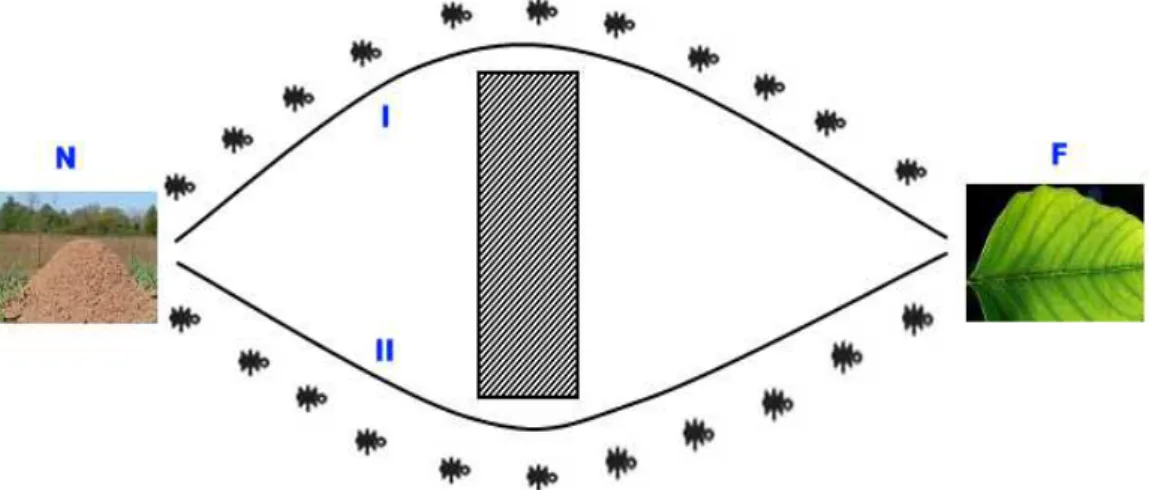
The behavior can be explained with the help of the following experiment. Consider the nest N and the point F where there is a source of food. Assume that there is an obstacle as shown in the Figure 1.1, between N and F, and the obstacle is symmetrically placed. Assume that at a given time t, equal number of ants have chosen the paths I, and II. Thus, the pheromone laid and the evaporation would be the same for the two paths. A new ant, starting from N, then would have equal chances for choosing paths I and II. If by chance, for a given period, the choices for one path dominate the other, then most probably, one path will gain more and more importance, disadvantaging the other one. For such a case, after some time, there would be no ants (or a few) preferring the chanceless path.

(21)

4

Figure 1.1 : Ants Foraging on Two Equal Paths

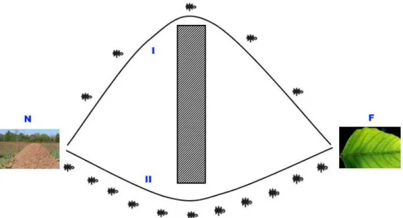
On the other hand, if the obstacle is unsymmetrical as shown in the Figure 1.2, the situation would be quite different. Assume again that at a given time t, equal amounts of ants have chosen paths I and II. At this time the pheromone density on the shorter path II will be higher than the path I, because of evaporation due to longer travel time on the route NFN. Thus, the new ant starting at N would more probably choose the shorter path II, thus increasing the importance of path II. So, as time goes on, path II will become more and more attractive and path I will be almost completely forgotten.

(22)

5

Figure 1.2 : Ants Foraging on Two Unequal Paths

This experiment shows that using very simple principles, ants show an ability of optimizing their route. This optimization process can further be improved by artificially playing with the amount of pheromone laid on the track as a function of the performance of the ant. This artificial process can better be understood considering the following case. Assume there are paths p1, p2,…., pK that are followed by K ants at a given move at a given time and p1 is better than p2, p2 is better than p3, etc. Then one can assume that the total pheromone distributed by ant following path p1 will be greater than that following p2, and so on. This consideration adds the following rule to the three rules given above: Total amount of pheromone distributed by an ant is proportional to its performance.

(23)

6

2. PREVIOUS APPLICATIONS IN LITERATURE

Ant colony optimization algorithms have been used to produce near-optimal solutions to the traveling salesman problem. They have an advantage over simulated annealing and genetic algorithm approaches when the graph may change dynamically; the ant colony algorithm can be run continuously and adapt to changes in real time. This is of interest in network routing and urban transportation systems.

Note that all of the problems above are discrete and related to graph theory and/or combinatorial problems. In this study, Traveling Salesman Problem (Dorigo and Gambardella 1997) will be solved using Ant Colony Optimization for demonstration.

2.1.TRAVELING SALESMAN PROBLEM

Although it seems to be difficult to see how these simple rules can be of use in solving complex optimizations problems, the literature is getting full of solutions obtained by ACO method and its variances. It has first been applied to Traveling Salesman Problem, which is a discrete optimization problem. In this problem the question is to find the shortest path that passes through all given discrete points without passing through a point more than once.

The method can be explained using the example given below which is the TSP with 5 nodes.

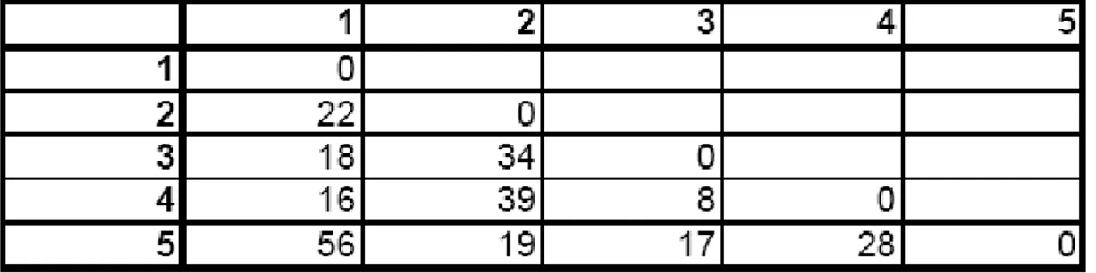
The Table 2.1 shows the distances between the cities, numbered from 1 to 5. There are empty cells since the distance from a city A to city B is no different than distance from B to A.

(24)

7

Table 2.1 : Distances between Cities for TSP

Figure 2.1 : Alternative Paths for the TSP

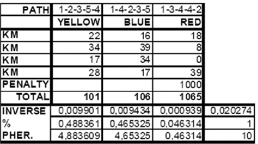
Foraging ants are selecting 3 paths as shown in the Figure 2.1. The Figure 2.2 shows the chosen paths in detail. If we are considering the yellow path, the number 22 in the Figure 2.2 shows the distance from city 1 to city 2. The number 34 is the distance from city 2 to city 3. The number 17 is the distance from city 3 to city 5. The number 28 is the distance from city 5 to city 4, and so on. The ant will be traveled 101 KMs total. The distance (cost) of the blue path will be 106. The red path is a special case. It passes from the city 4 more than once. Note that this can be avoided by forbidding, or using a penalty point. In this example, the penalty point method has been chosen. The number 1000 stands for the penalty point given for the red path. After applying the penalty, the total cost of the red path will be 1065, which means that this path is worse than the other two.

(25)

8

Figure 2.2 : Cost of the Paths for TSP

The amount of pheromone to be added to the artificial map is seen at the bottom of the Figure 2.2. The better path must have more pheromone. To provide this artificially, the inverse of the total cost will be used as a pheromone amount. In this case, the yellow path will deserve more pheromone, the blue path will deserve a bit less, and the red path will get much less pheromone than the other two. Any successor ant is likely to choose the yellow path or the blue path since they will be more attractive because of their rich pheromone scent. Meanwhile the chance of the red path is much lower than the others.

(26)

9

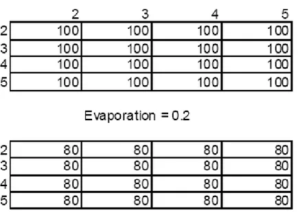
Figure 2.3 : Evaporation on the Paths of TSP

The evaporation is shown in the Figure 2.3. To make the evaporation artificially, a constant is chosen, 0.2 in this case. If the cells have pheromone of 100, they will contain 80 after the evaporation.

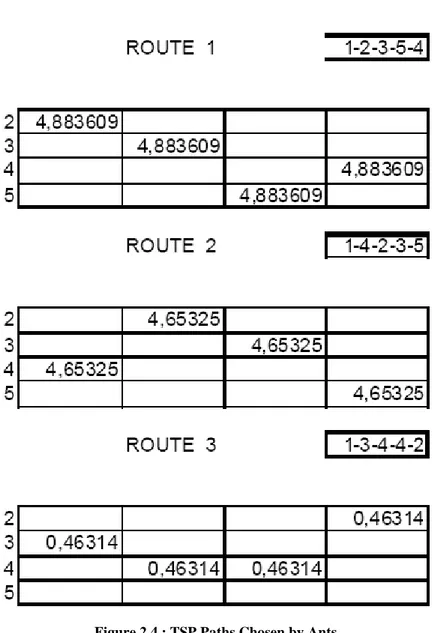
The Figure 2.4 shows the movements of the 3 ants. Using the calculated pheromone amounts by the Figure 2.2, the values are added to the solution map. Continuing from the state evaporation state, the state of the map will be as in the Figure 2.5.

(27)

10

Figure 2.4 : TSP Paths Chosen by Ants

(28)

11

3. TRUSSES

Structures can be considered of three basic types:

i. Structures made of bars (Beams, columns, trusses, frames) ii. Structures made of surfaces (Plates, shells, domes)

iii. Structures of volume type (Earth, tunnels, dams)

Trusses are structures made of solid bars which are called “members” or “elements”. Members are joined to each other at “nodes” or “joints” which are free to rotate, that is with no resistance to member rotations. In other words there are no moments at joints.

One primordial assumption about trusses is that the loads are applied only at joints. This assumption results in the fact that the forces in the members are axial only; they are either tension or compression. In structural engineering convention, tensile forces are accepted as positive, compressive forces are said to be negative (Toklu 2004).

Trusses can be in a plane, which are called “plane trusses”, or they can be 3-dimensional, which are called “space trusses”.

The joints can be free to move under the action of applied loads, or some or all of their displacements can be restricted. Joints with restricted displacements are called “supports”. For example, the displacements of a joint in a space truss can be restricted in z direction and free to move in x and y directions. In this case, it will be understood that there is a “support reaction” at that joint in z direction to make the displacements zero in that direction (Toklu 2004).

To solve or to analyze a truss means to determine all joint displacements, member forces and support reactions. This is not very difficult in the linear range. The most advanced technique used for this purpose is the well known “Finite Element Method” which results

(29)

12

in a matrix formulation like Kx = b, Here K is a square matrix called “stiffness matrix” presenting material and geometric properties of the truss. x is a column vector of joint displacements, b is another column vector giving the loads applied at joints. When the x is solved from this equation by any method for solving simultaneous linear equations, the forces in members and reactions at supports can be found from simple static equilibrium equations. (Toklu 2004)

Trusses enter into nonlinear range in two cases:

i. Material nonlinearity. The material with which the members are made of can be nonlinear. Common examples to this case are plastic or elasto-plastic materials.

ii. Geometrical nonlinearity. The above equation Kx = b, can be written with no great difficulty, if the displacements are so small that they can be neglected in comparison to truss dimensions. If the displacements are large, then again it is not possible to write this basic equation.

A truss can be nonlinear if there is material nonlinearity, geometrical nonlinearity, or a combination of them. In such a case the only method used until now is piecewise linearization which inevitably introduces errors to the solution (Toklu 2004).

3.1.DISSECTION OF A TRUSS FILE

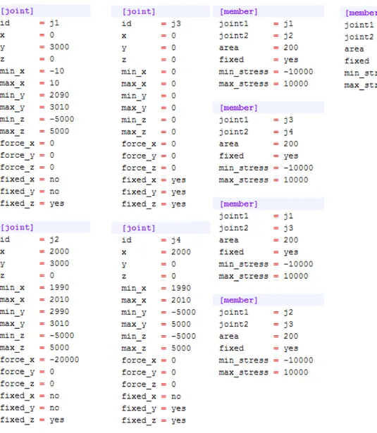
The trusses are introduced to the Truss Solver using input data files in text format. The example file given below in the Figure 3.1 represents a truss with four joints and five members. The content of this file is read by the program using the FlowReader library. In this file first the joint data is given. This is followed by member data.

(30)

13

Figure 3.1 : A Truss File Example

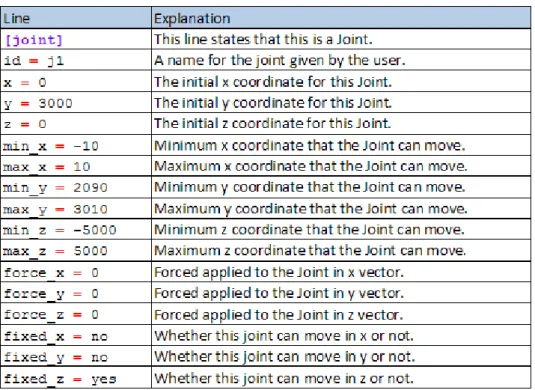
3.2.DISSECTION OF A JOINT

(31)

14

Table 3.1 : A Joint

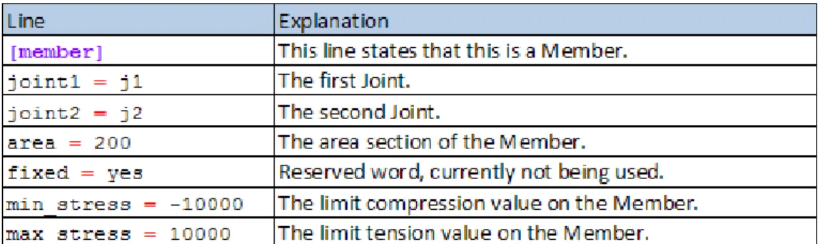
3.3.DISSECTION OF A MEMBER

Dissection of a member is seen in the Table 3.2. Members are placed between two Joints. The input file states that by using the joint1 and joint2 tags.

The minimum stress is the value that this member can stand against compression. The maximum stress is tension that this member can stand against. Values outside of the range [min_stress, max_stress] will cause deformation on the member, thus, should not be allowed. Throughout the program, paths causing values outside of this range are given a special penalty point taking them far away from the best path.

(32)

15

Table 3.2 : A Member

3.4.MINIMUM ENERGY PRINCIPLE

The principle of minimum total potential energy is a fundamental concept used in science and engineering based on the observations from nature. It asserts that a structure or body shall deform or displace to a position that minimizes the total potential energy. For example, a ball placed in a bowl will move to the bottom and rest there, and similarly, water will flow downwards as long as it finds a way to itself (Toklu 2004).

Note that in most complex systems there is one global minimum and many local minima (smaller dips) in the potential energy. A system may reside in a local minimum for a long time - even an effectively infinite period of time. An algorithm intended to find the global minimum can easily be unsuccessful but getting stuck in a local minimum (Toklu 2004).

The principle, in usually accepted way, can be restated as: "Of all the displacements which satisfy the restrictions on joint displacements of a structural system, those corresponding to the stable equilibrium configurations make the potential energy a relative minimum". This principle, although well known and applied through illustrative examples in almost every structural analysis book, is not thoroughly exploited except for very few cases (Toklu 2004).

(33)

16

3.5.ENERGY OF A TRUSS

Total potential energy of a truss can be found as the algebraic summation of the strain energy in the members and the work done (negative) by the loads applied at joints. The total potential U for a given state of deformations (characterized by the strains ε within the body, creating the generalized deflections ui coupled with the generalized loads Pi) can be

written as Equation 3.1

∫

∑

= − = NP i i i V u P dV e U 1 ) ( ) (ε ε Equation 3.2 =

∫

ε ε ε σ ε 0 ) ( ) ( d e where

σ and ε are stress and strain which are interrelated through σ = σ (ε), e is the strain energy density,

NP is the number of loads,

V is the volume of the body.

For a given material the stress strain relation σ = σ (ε) is assumed to be completely known and thus it will be possible to determine the integrals in the above equations. In this study, elastic materials are considered so that = Eε where E is the modulus of elasticity of the material (Toklu 2004).

Consider a plane truss with Nm prismatic members, Nj joints and NP loads. Consider the

element ij (see the Figure 3.2) with original end coordinates (xi, yi) and (xj, yj) and with

original length

(34)

17

Figure 3.2 : Displacement of Joints and Members

After end displacements (ui, vi) and (uj, vj) corresponding to a configuration c, the final

length will be

Equation 3.4 L(c) = ((xj-xi + uj-ui)2 + (yj-yi + vj-vi)2)1/2

where c = [c1 c2 … c2Nm]T = [u1 v1 u2 v2 … uNm vNm]T represent the displaced configuration

of the structure. The elongation of the member considered then is ∆L(c) = L(c) - L(0) and the strain is ε(c) = ∆L(c) / L(0). It can be seen that if the end displacements are known, then strain for each member can thereof be determined. , Then the integral in (2) can be taken for each member to yield ej, j =1, …,Nm. Since the volume of an original truss element is

AjLj, then energy takes the form

Equation 3.5

∑

= = − = m NP i i i N j j j jA L Pu e U 1 1 ) (ε

The problem then is to determine the vector c = [ u1, v1, …, uNj, vNj]T satisfying joint

fixities and minimizing U (Toklu 2004). y, v j' vj i' vi j uj i ui x, u

(35)

18

4. LIBRARIES AND TOOLS USED

4.1.PSYCO PYTHON EXTENSION

Psyco is a Python extension module which can massively speed up the execution of any Python code. The average speed improvement is approximately 4x, making Python performance close to compiled languages. In very rare cases, it can speed up to 40x.

In this study, Psyco has been extensively used to improve the performance.

4.2.IRONPYTHON

IronPython is an implementation of the Python programming language, targeting the .NET Framework and Mono, created by Jim Hugunin. It supports an interactive console with fully dynamic compilation. It is well integrated with the rest of the .NET Framework and makes all .NET libraries easily available to Python programmers, while maintaining full compatibility with the Python language. Another advantage of making the code compatible with IronPython implementation is to be able to use the fully static compilation of the code to .NET platform.

IronPython is written entirely in C#, although some of its code is automatically generated by a code generator written in Python.

4.3.MERSENNE TWISTER PSEUDORANDOM GENERATOR

The Mersenne Twister is a pseudorandom number generator developed in 1997 by Makoto Matsumoto and Takuji Nishimura that is based on a matrix linear recurrence over a finite binary field F2. It provides for fast generation of very high-quality pseudorandom numbers,

(36)

19

having been designed specifically to rectify many of the flaws found in older algorithms (Matsumoto and Nishimura 1998).

It was designed to have a period of 219937 − 1 (the creators of the algorithm proved this property). In practice, there is little reason to use larger ones, as most applications do not require 219937 unique combinations (219937 is approximately 4.315425 × 106001) (Matsumoto and Nishimura 1998).

The code in the Figure 4.1 produces the output in the Figure 4.2. This shows the relatively long period of the Mersenne Twister algorithm.

(37)

20

(38)

21

5. METHOD OF SOLUTION

5.1.PANTS LIBRARY

It is short for “Python Ants”. It is fully developed in Python for code clarity. It is both 32-bit and 64-32-bit compatible allowing the program to be run under high performance servers and super computers. Although Python is an interpreted language and not as fast as compiled languages like C or C++, it can be optimized by Just-in-Time compilation using tools like Psyco.

The library has also a compatibility layer with IronPython, allowing the code to be statically compiled as a .NET DLL. Although the Python itself is running flawlessly under Windows environments, there is another advantage of using a .NET DLL: To allow other programs to use the library, and expanding the solution family of the library.

The library itself is independent of the problem. The same library has been used to solve the Rosen’s Function to Minimize and various truss energy minimization problems. Any external code can use the pants library to use an appropriate problem.

The library includes:

i. The class Ant

ii. The class AntVariable iii. The class AntMap iv. Exception classes :

a. MinimumConstraintIsGreaterThenMaximumConstraintException b. InvalidClassAttributeException

c. InvalidTypeException d. NotAFunctionException,

(39)

22 e. KValueCannotBeZeroException f. KValueCannotBeLessThanZeroException g. PointsCannotBeZeroException h. PointsCannotBeLessThanZeroException i. OtherObjectInstancesInAntVariablesList j. FileAlreadyExistsException

v. IronPython compatibility layer vi. The class SelectionWheel vii. IronPython Compatilibity

(40)

23

5.2.SELECTION WHEEL MODULE

Figure 5.1 : SelectionWheel Members

The Selection Wheel module includes the class SelectionWheel. The structure of the class SelectionWheel can be seen in the Figure 5.1. This class is responsible of choosing an item among alternatives according to their chances. Each item is called as competitor throughout the program. The competitors are added using the function addCompetitor and the share of their chances. After all the competitors as been added to an instance of a SelectionWheel, the wheel is being driven and one of the competitors is selected among them.

(41)

24

Figure 5.2 : SelectionWheel Example

In a simple demonstration as the Figure 5.2 states, there are 4 competitors, with 4 different names. Note that the share for competitor white is 0. This is one of the special cases that the class SelectionWheel must stand. A competitor with 0 share will have no chance to be chosen. To avoid this, SelectionWheel applies the threshold by automatically using the function __findMinimumNonZeroShare(). This function will find the competitor with the

(42)

25

minimum nonzero share, the competitor blue with the share of 5, in this case. The share of 5 is given to the competitor white too. Note that this will not reflected to the real pheromone amount in the map, leaving everything as it is. Finally, the competitor white will have a chance of 5/40, the competitor red will have a chance of 20/40, the competitor green will have a chance of 10/40 and the competitor blue will have a chance of 5/40 respectively. The output of this simple demonstration is seen at the bottom of the Figure 5.2. This states that, even though a competitor has a chance of zero, there will be chance to be selected, avoiding one of the biggest risks in metaheuristics algorithms; being stuck in local optimum.

Another difficulty that the SelectionWheel must solve is the case that all of the competitors have a chance of 0. In this case, a threshold is applied, giving all of them the same number of points for a fair competition and choosing one of them. This case can occur when the first ant of the first colony walks. Since there no any successor ant before the first, there can be no pheromone on the map. This case can be overcome by setting a default pheromone amount in the instantiation of the class AntMap, to improve performance.

By avoiding these two cases, the class SelectionWheel chooses one of the competitors fairly.

This module depends on the Mersenne Twister pseudorandom generator for random numbers.

(43)

26

5.3.FLOW READER MODULE

Figure 5.3 : FlowReader Members

As the Figure 5.3 shows, the module Flow Reader includes 4 exception classes and the class FlowReader. It is used to read flowing stream like reading from a list. Unlike sequentially reading, which is stateless, the FlowReader is stateful. Its main purpose is to read input data files object by object.

The function __init__() is called with a file name, which is supposed to be a truss file. The file then read into memory and the caller can pull the objects of Joint and Member one by one without getting all of them if it is not required.

The function resetCursor() is used to reset the cursor, initializing the read state to the beginning. The function getNext() returns the next line. The function getUntil() takes one

(44)

27

parameter which the last item demanded. When it is called, it stacks the items, and returns the stack until the parameter is reached. This provides great advantages for reading stateful truss objects.

5.4.ANTS MODULE

The module Ants includes 3 important classes, AntVariable, AntMap and the Ant. It is independent of the problem.

5.5.ANT VARIABLE

Since the module has been specifically designed to solve continuous problems, an instance of an AntVariable represents an unknown in an equation. More than one AntVariable instance can be placed into an AntMap to solve complex problems. The Figure 5.4 shows the members of the class AntVariable.

(45)

28

Figure 5.4 : AntVarible Members

The attribute var_name stands for the variable name assigned by user name to track down its changes. The unnormalized_min and unnormalized_max are used to keep the variables’ orginal constraints. The variable then will be normalized, and, the normalized state will be kept in the pair of normalized_min and normalized_max attributes. The attribute normalization_delta is used for the difference in the moralization operation, as it will be explained in details. The global_min and global_max keeps the first original constraints of the variable, since the others will be modified throughout the iterations of the adaptive solutions, but the first original constraints will be kept no matter what. The attribute digits_after_dot used for precision. The attribute initial_ant_trails is the amount of pheromone to be put initially. The attribute variable_pheromones is the actual list of the

(46)

29

pheromons. And finally, the ant_trails_time_factor is the factor to evaporate the pheromones from the map.

The Figure 5.5 shows an arbitrary ant variable, x1, in the discretized form. If an ant to choose the specified path as in the Figure 5.5, this would give the result, 0.053574 which is to be unnormalized in the next step. The variable in the Figure 5.5 is discretized with 6 digits after dot.

Figure 5.5 Demonstration of an Ant Variable

5.5.1. Normalization

ACO is especially useful to solve discrete problems (Dorigo et al. 1999). To discretize a continuous variable, the class AntVariable uses a special method, normalization. In an equation, a variable can have constraints such as in the case of Rosen’s Function (Colaco et al. 2005) and the Truss problem (Toklu 2004).

(47)

30

If the variables’ constraint is 50<x<200, the normalization delta will be -50. Then, this value is added to both unnormalized_min and unnormalized_max, bounding the variable x between 0 and 150, as applied in the Figure 5.6. If the constraint is negative, at least one of them, as in the example of -50<x<100. In this case, the delta will be +50, and the boundaries will be 0<x<150.

Figure 5.6 : Normalization Algorithm

The normalization operation is specific to each instance of AntVariable. Two variables with different constraints can live together without affecting each other.

The backwards operation which is getting the real, continuous value from a path is done as in the Figure 5.7.

Figure 5.7 : Discrete to Continuous Conversion Algorithm

In the Figure 5.7, the path walked is a string holding the digits chosen by the ant.

5.5.2. Digits after Dot

The attribute digits_after_dot is the amount of precision. If the value is greater, the precision will be improved but it will consume more time and require more process power.

(48)

31

Since the problem is being attacked in the discretized form, even though it is continuous, the attribute digits_after_dot is enlarges the solution map.

To overcome the difficulties occurred when demanding more precision without requiring too much processing power, an Adaptive Solution method is introduced later in this chapter.

The digits after dot can be seen in the Figure 5.5. In that case, the value of digits_after_dot is 6.

5.5.3. Variable Pheromones

This is the list of actual pheromones for the variable. This array will include other arrays of count digit digits_after_dot. When evaporation occurs, all of the values in variable pheromone array will be multiplied by a specific evaporation factor. When an ant has finished walking, all paths ant walked is increased by the amount of pheromone calculated by the phi function. It is the number of columns in the Figure 5.5.

5.5.4. Initial Ant Trails

In nature, if a path is not discovered, there will be no pheromone scent on it. In this implementation, one can specify an amount of initial ant trails for performance reasons. If the number is large enough that it will not exhaust after all of the iterations, this will improve the performance since it lowers the count of floating point operations. It will also avoid depending on selection wheel’s “give a chance to the competitor with zero share” feature.

Another crucial functionality of initial ant trails is to provide the fairness among the alternative paths. If the first ant in the first colony were to choose a path while all the others

(49)

32

have no pheromone at all, the following ants were very likely to choose that path. To overcome that, the Selection Wheel would play a role, but, in that case, the first path would have an equal chance to be selected with the others while it has to have a bit more chance than the others. The initial ant trails provides a way from escaping this problem.

5.5.5. Evaporation

After each iteration, the pheromones tend to evaporate. It is a fade out, and it lowers the amount of pheromone on the map. It is decreased by the factor ant_trails_time_factor which is the evaporation factor so they will never reach to zero and the selections among paths will be as fair as it gets. The algorithm can be seen in the Figure 5.8.

Figure 5.8 : Evaporation Algorithm

The evaporation avoids a very critical case: The domination of a specific path over others. By evaporating the pheromone scents by a specific factor, no path will dominate the others while keeping the advantage among them.

A better path will get better naturally, since a shorter path (which means a better solution in ACO) is marched faster and keeps more pheromone scent on itself.

5.5.6. Adding Pheromones

After each iteration, the amount of pheromones are added to the path marched. Each discrete cell on the map will get the same amount of pheromone calculated for that path. The same cell can get a higher amount of pheromone if the path is relatively good, or very

(50)

33

less amount of pheromone if the path is relatively bad. The algorithm to add the pheromones can be seen in the Figure 5.9.

Figure 5.9 : Adding Pheromone Algorithm

5.5.7. Extracting the Real Value of the Path

The data is kept in discrete form. To get the real value from the AntVariable object, it is unnormalized back. The algorithm can be seen in the Figure 5.10. In this case, walked_path is a string, “340763” for instance. The algorithm converts the path notation into the real value that can directly be used in the original equation of the problem.

.

Figure 5.10 : Unnormalization Algorithm

5.5.8. Adaptive Solution

The adaptive solution brings the performance facilities to the problem and it allows discovering solutions with higher precision. The variable shrink_factor is set in the AntMap. In the current implementation, it has been used as 0.8, which shrinks a little. Lower values like 0.2 has shortened the solution time, but had an impact on escaping from a local optimum.

(51)

34

As stated in the Figure 5.11, this algorithm is used to shrink the boundaries of the normalization values of the solution space. By this method, the problem can be solved over and over, using the best and worst solution in the previous solution.

Figure 5.11 : Shrinking Algorithm

The shrinking operation is applied to each AntVariable instance separately by examining the solution in the previous iteration. This provides escaping a steady-close variable losing its boundaries by the affect of a quickly changing variable.

5.6.ANT MAP

The AntMap class is used to add instances of AntVariable class to the solution space. It is also responsible of setting initial values, binding evaluation function using a function pointer, marching ant colonies, marching ants, solving the problem and returning the result. It is the main class in the library.

An AntMap is used to keep the instances of AntVariables and other environmental variables such as the phi values and its relation information. A demonstration of an AntMap is shown in the Figure 5.12 which includes n AntVariables.

(52)

35

Figure 5.12 : A Demonstration of an AntMap

(53)

36

(54)

37

5.6.1. Phi Function

Phi function is the evaluation function for the pants library. It is completely problem specific. It is bound to the library using a function pointer. This allows adopting different problems from different families to be solved using the method of solution. The values extracted from the path are sent to the phi function and the function returns a result. It is this function to be used to calculate the pheromone amount for the path. The Figure 5.14 shows the parameter initialization and calling the phi function and getting the function result in return.

Figure 5.14 : Dynamic Phi Function Calling Algorithm

5.6.2. Setting Initial Values for Phi Function

The amount of pheromone amount deserved by a path should be relational to the others. But, initially, there is no path known to state that relation. In this case, the first colony is responsible of marching the map and setting some constants that will to establish the relation. Since there is no any pheromone scent on the map, the first colony will walk randomly.

(55)

38

Two variables must be set while initializing the AntMap class. These are default_points_for_best and default_points_for_worst. These are arbitrary constant values and will not change in the programs’ lifetime, to protect the relation. In this study, default_points_for_best is chosen as 200 and default_points_for_worst is 100.

Then, the program must find the best and worst among the first colony, the one marched without sensing any pheromone scent, thus, fully random.

Figure 5.15 : Finding the Maximum and Minimum Phi Algorithm

The Figure 5.15 shows the algorithm to find the maximum and minimum phi values. The program then calculates the k-value and phi_0, which is constant phi calculated from the

(56)

39

first iteration. These two values will be then referenced every time phi value for a path is calculated. The Figure 5.16 shows the algorithm.

Figure 5.16 : Calculating k-value and phi_0 Algorithm

The phi value for chosen path of any following ant can be then calculated as in the Figure 5.17.

Figure 5.17 : Algorithm to Calculate Phi Value for an Ant

.

5.6.3. Maximization or Minimization Problem

The study can solve both minimization and maximization problems. Internally, the program is always using minimization. If the problem is a maximization problem, the terms are multiplied by -1, and it is minimized. The program is multiplying every result and phi value by phi_factor. If the problem is a minimization problem, the phi_factor will be 1, which does not affect the results. But, if it is a maximization problem, the phi_factor will be -1 as in the Figure 5.18.

(57)

40

5.6.4. Adding Ant Variables

The AntMap class keeps the instances of AntVariables. The number of variables is not limited; it can vary from a few as in Rosen’s Function, or, much more as in the Truss problems. Ant number of variables can be added.

5.6.5. Foraging Ant

An ant instance walks on the map while foraging. The amounts of pheromones are given as competitors to the Selection Wheel as in the Figure 5.19. Note that the same instance of SelectionWheel is used for all ants for performance reasons. Each time an ant walks, the SelectionWheel is reset clearing previous competitors. Selection Wheel returns the selected one, and it is added to the path. When the ant finished marching the map, the phi value for the path is calculated.

(58)

41

5.7.ANT

An Ant instance is used to keep the walked path and corresponding phi value as a whole. It also includes the colony no and ant no, to track down the results. In addition, the best ant is always kept in the memory until an even better one is found. The purpose behind keeping the number and colony of the best ant is to examine the improvement in the solution. It is likely be one of the latest ants since the initial ants have walked randomly, but the following ants depended on the previous ones. The members of an Ant object can be seen in the Figure 5.20.

Figure 5.20 : Ant Members

5.8.ANT COLONY

An ant colony is a group of ants, marching in parallel. This is very crucial to avoid the ants to choose the same path over and over. In nature two ants going on the different directions will not affect each other. But, in this study which applies discrete solution methods to continuous problems, each node is connected to each other. So, the path chosen by the first ant will have an advantage over others, and, if it is a bad path, it will lower the chances of selection of better paths. To avoid this problem, ants made walk in groups. Only after all

(59)

42

the ants in a group, which is called a colony in this study, finished walking, the pheromone amount for each of the ant is calculated, and committed to the map. The algorithm can be seen in the Figure 5.21.

Figure 5.21 : Ant Colony Algorithm

5.9.SOLVING ROSEN’S FUNCTION TO MAXIMIZE

To demonstrate the program, a relatively simpler function, Rosen’s Function to Maximize is to be solved (Colaco et al. 2005).

(60)

43

As can be seen from the Figure 5.22, the function has 8 terms, 2 variables and it is to be maximized. All of this information is required to be provided to the library.

The pants library has been used to solve this problem with ACO.

The first step is to adapt the problem to the solver. To achieve this, the evaluation function (the function to be used to calculate phi values of the chosen paths) is provided as in the Figure 5.23.

Figure 5.23 : Evaluation function for Rosen

The next step is to introduce the variables x1 and x2 to the program as in the Figure 5.24 and the Figure 5.25. Please note that the information about the constraints is provided to the variable to enable the discretizaton and normalization.

(61)

44

Figure 5.24 : The variable x1 of Rosen

Figure 5.25 : The variable x2 of Rosen

The next step is to put these two variables to an AntMap and initialize it as in the Figure 5.26.

(62)

45

Figure 5.26 : The map of Rosen

Since it is a maximization problem, it is stated. In this solution attempt, 100 colonies and 100 ants per colony have been used, giving totally 10000 ants.

The program give the results in the Figure 5.27 after 121 seconds (on a computer with 1 GB RAM, Pentium 4 2679 MHz).

Figure 5.27 : Result of Rosen’s Function

5.9.1. Shrinking in Adaptive Solution

To demonstrate the shrinking for adaptive solution, the boundaries for one of the variables, x1, will be shown here. Although the constraints for x1 and x2 are equal to each other, boundaries are affected by the ants, as a result, they are not the same but similar. The Figure 5.28 shows the changes about boundaries occurred on the variable x1.

(63)

46

Figure 5.28 : Shrink on x1 of Rosen

5.10. SOLVING A TRUSS

5.10.1.Input Data

The problem to be used in the demonstration is the file introduced in the Figure 3.1. The Figure 5.29 shows its visualized form.

(64)

47

Figure 5.29 : Visualization of the Truss File

5.10.2.Placing Data into the AntMap

Although the problem being solved is a plane truss (2D), the library supports both 2D and 3D (space truss) problems. The coordinates of joints are placed into the AntMap. A joint can be fixed in a dimension, but can be put on a roller in another one. For example, in the Figure 3.1, the joint j1 can move on x and y, but it is fixed in z. In this case, only x and y coordinates are placed into the AntMap to save the process power.

(65)

48

Figure 5.30 : Algorithm to Create Variables from Joints

When the Truss displaces, its state can easily be obtained from the AntMap.

For this problem, the program creates 5 variables to place into the AntMap, which are x and y coordinates of joint j1, x and y coordinates of joint j2 and x coordinate of joint j4. As stated, fixed coordinates are not placed into the AntMap.

5.10.3.Phi Function for Truss Displacement

Fitness of a truss can be calculated as in the Figure 5.31. The fitness of a truss is considered as a whole, for the truss. Since this is the minimization problem, higher amount of energy is considered against the fitness; as a result, they are positive. Members are placed between joints. If two joint are to displace, the member deforms. The material of the member has some limits obviously, and cannot be expected to take the shape of every case. A penalty can be applied if a member is out of boundaries. The penalty point is against the fitness; as

(66)

49

a result, it is positive. The last term in calculating the fitness is the work done by each joint (Toklu 2004).

Figure 5.31 : Algorithm to Calculate Fitness of a Truss State

The strain energy can be calculated as in the Figure 5.32. The original state of the truss is never disposed in the life time of the program so that the original length of a member can always be used, and strain for a member can always be calculated. The E_FACTOR is a material constant and depends on the material used (Toklu 2004).

Figure 5.32 : Algorithm to Calculate Strain Energy

The work done can be calculated as in the Figure 5.33. The original position, which is always kept in the memory, is used to calculate the work done by a joint, using vector algebra.

(67)

50

5.10.4.Result

The results found can be shown as follows:

[('j1.x', -9.2366572364787114), ('j1.y', 2999.9869519939502), ('j2.x',

1990.762667928311), ('j2.y', 3002.2411931278461), ('j4.x', 1999.996501008251), ('phi', -92312.918205940572)]

(68)

51

6. CONCLUSIONS AND FUTURE STUDIES

Use of energy minimization for analysis of structures is a technique which is becoming popular in these years. For very long times, this technique is known to be theoretically possible, but practically very difficult to apply. Only very recently, with the advances in metaheuristic optimization methods and with the advances in computer technology, in capacity, speed, and new software possibilities, applications of this method have seen the day. Until now very few structures are analyzed in this way, all of them being trusses. The metaheuristic method tried for this purpose was the random search optimization method. It has been shown in this study that Ant Colony Optimization (ACO) also can be applied to the problem.

ACO is a method which is originally designed for solving combinatorial or discrete optimization problems. That is why it has found applicability especially in the field of discrete problems. ACO applications for continuous problems are very rare and still at the stage of development. For such problems it is almost always applied using binary number system. In this study, it has been shown that it can also be applied using decimal number system.

ACO method is based on very simple principles, learned and adapted from real life. It is interesting to see that with such simple principles one can solve very complex problems, which are otherwise very difficult to solve. To show and guarantee the applicability of solving continuous problems using ACO method, the first problem attacked in this study was the optimization of functions taken from literature. Only after the success of this application the truss problem is attacked.

Analysis of trusses in the range of linearity do not pose important difficulties. Using force method, or finite element methods, trusses can be analyzed in this range under the assumption that the deformations are infinitesimal so that the free body diagrams can be drawn taking the undeformed geometry of the structure. But if the deformations are large, it

(69)

52

is no longer possible to draw the free body diagrams based on the original shape, thus the problem becomes nonlinear. The solution technique for these cases is to use iterations, or partial iterations. Such techniques are very cumbersome to apply and are always bound to include errors.

The optimization method used in this analysis have shown that such nonlinear problems can be solved using this combination of ACO and energy minimization technique. The only drawback of the method is the high number of ants to be let to find the correct solution for the given problems. This is the general situation for ACO applications both in natural life and in artificial life. It must not be forgotten that if a solution is being obtained to a problem which is otherwise almost impossible to solve, than time does not matter.

The study presented here can further be advanced in many directions.

i. Other metaheuristic methods can be applied to the same problem to find the most effective one among them.

ii. The method used can be developed to solve other types of optimization problems. iii. The method can be generalized to be applicable to nonlinear materials to include for

example elasto-plastic materials.

iv. With some more structural engineering inputs, the method can be generalized to solve other types of structures, like plates, shells, etc.

v. A thorough investigation on the parameters and modifications of ACO can be made to optimize the method. An example can be the comparison of the efficiencies of binary, decimal, and hexadecimal number systems.

(70)

53

REFERENCES

Books

Dorigo, M., Stützle, T., 2004.. Ant Colony Optimization. MIT Press, Cambridge, MA. Bonabeau, E., Dorigo, M., Theraulaz, G., 1999. Swarm Intelligence: From Natural to

Artificial Systems, Oxford University Press.

Periodical Publications

TOKLU, Y.C., 2004. Nonlinear Analysis of Trusses Through Energy Minimization.

Computers and Structures, Vol. 82, pp.1581-1589.

Deneubourg, J.-L., Aron, S., Goss, S., Pasteels, J. M., 1990. The self-organizing

exploratory pattern of the Argentine ant. Journal of Insect Behavior, 3:159–168. Di Caro, G., Dorigo, M., 1998. AntNet: Distributed stigmergetic control for

communications networks. Journal of Artificial Intelligence Research, 9:317–365. Dorigo, M., Blum, C., 2005. Ant colony optimization theory: A survey. Theoretical

Computer Science, 344(2–3):243–278

Dorigo, M., Gambardella, L. M., 1997. Ant Colony System: A cooperative learning approach to the traveling salesman problem. IEEE Transactions on Evolutionary

Computation, 1(1):53–66.

Dorigo, M., Maniezzo, V., Colorni, A., 1996. Ant System: Optimization by a colony of cooperating agents. IEEE Transactions on Systems, Man, and Cybernetics – Part B, 26(1):29–41,.

Gutjahr, W. J., 2000. A Graph-based Ant System and its convergence. Future Generation

Computer Systems, 16(8):873–888.

Stützle, T., Hoos, H. H., 2000. MAX–MIN Ant System. Future Generation Computer

Systems, 16(8):889–914.

Dorigo, M., Di Caro, G., Gambardella, L. M.. 1999. Ant Algorithms for Discrete Optimization. Artificial Life, 5 (2): 137–172.

(71)

54

Colaco, M. J., Dulikravich, G. S., Orlande, H. R., Martin, T. J., 2005. Hybrid Optimization with Automatic Switching Among Optimization Algorithms. Evolutionary

Algorithms and Intelligent Tools in Engineering Optimization, pp. 92-118.

Matsumoto, M., Nishimura, T., 1998. Mersenne twister: a 623-dimensionally

equidistributed uniform pseudorandom number generator. ACM: Transactions on

Modeling and Computer Simulation, 8, 3.

Other Publications

Dorigo, M., 1992. Optimization, Learning and Natural Algorithms (in Italian). PhD thesis, Dipartimento di Elettronica, Politecnico di Milano, Milan, Italy, 1992.

Dorigo, M., 2007. Ant colony optimization. Scholarpedia, 2(3):1461

Dorigo, M., Maniezzo, V., Colorni, A., 1991. Positive feedback as a search strategy. Technical Report 91-016, Dipartimento di Elettronica, Politecnico di Milano. Bonabeau, E., Dorigo, M., Theraulaz, G., 2000. Inspiration for optimization from social

insect behavior. Nature;406:39–42.

Internet

Ant. 2008. http://en.wikipedia.org/wiki/Ant [cited September 2008]

Ant Colony Optimization. 2008. http://en.wikipedia.org/wiki/Ant_colony_optimization [cited September 2008]

(72)

55

CURRICULUM VITAE

Name Surname : Şakir Çağlar TOKLU

Address : TTG International Ltd

Dilek Sok.NO: 10 Kat: 3 Dikilitaş, 34349 Beşiktaş, Istanbul, Türkiye

Birth Place / Year : Ankara - 1979

Languages : Turkish (native), English, French

High School : Đzmir Buca Anatolian High School - 1997

BSc : TRNC Eastern Mediterranean University - 2004

MSc : Bahçeşehir University – 2008

Name of Institute : Institute of Science

Name of Program : Computer Engineering

Publications :

Work Experience : 2008 May - …

Software Developer TTG International 2006 Sept – 2008 May

Teaching and Research Assistant

Bahçesehir University Software Engineering Department 2005 Jan – 2005 July

Software Developer Bizitek

Nonlinear displacement analysis of trusses using ant colony optimization

T.C.

B A H Ç E Ş E H Đ R Ü N Đ V E R S Đ T E S Đ

NONLINEAR DISPLACEMENT ANALYSIS OF TRUSSES

USING ANT COLONY OPTIMIZATION

Graduation Thesis

Ş

AKĐR ÇAĞLAR TOKLU

T.C.

B A H Ç E Ş E H Đ R Ü N Đ V E R S Đ T E S Đ

THE INSTITUTE OF SCIENCE

COMPUTER ENGINEERING

NONLINEAR DISPLACEMENT ANALYSIS OF TRUSSES

USING ANT COLONY OPTIMIZATION

Graduation Thesis

Ş

AKĐR ÇAĞLAR TOKLU

Supervisor : PROF. DR. NĐZAMETTĐN AYDIN

Co-Supervisor : DOÇ. DR. YUSUF CENGĐZ TOKLU

T.C.

B A H Ç E Ş E H Đ R Ü N Đ V E R S Đ T E S Đ

INSTITUTE OF SCIENCE

COMPUTER ENGINEERING

ACKNOWLEDGEMENTS

ABSTRACT

ÖZET

TABLE OF CONTENTS

LIST OF TABLES

LIST OF FIGURES

LIST OF EQUATIONS

∫

∑

∫

∑

∑

LIST OF ABBREVIATIONS

LIST OF SYMBOLS

1.

INTRODUCTION

2.

PREVIOUS APPLICATIONS IN LITERATURE

3.

TRUSSES

∫

∑

∫

∑

∑

4.

LIBRARIES AND TOOLS USED

5.

METHOD OF SOLUTION

6.

CONCLUSIONS AND FUTURE STUDIES

REFERENCES

CURRICULUM VITAE