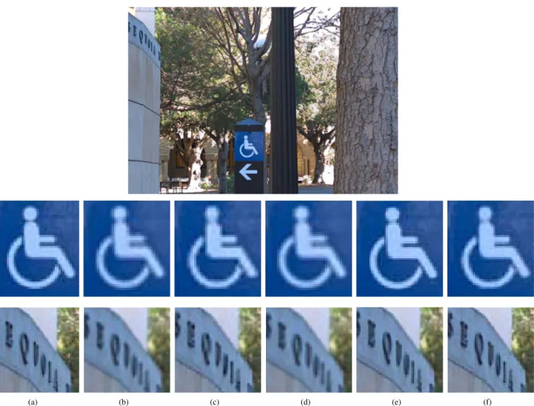
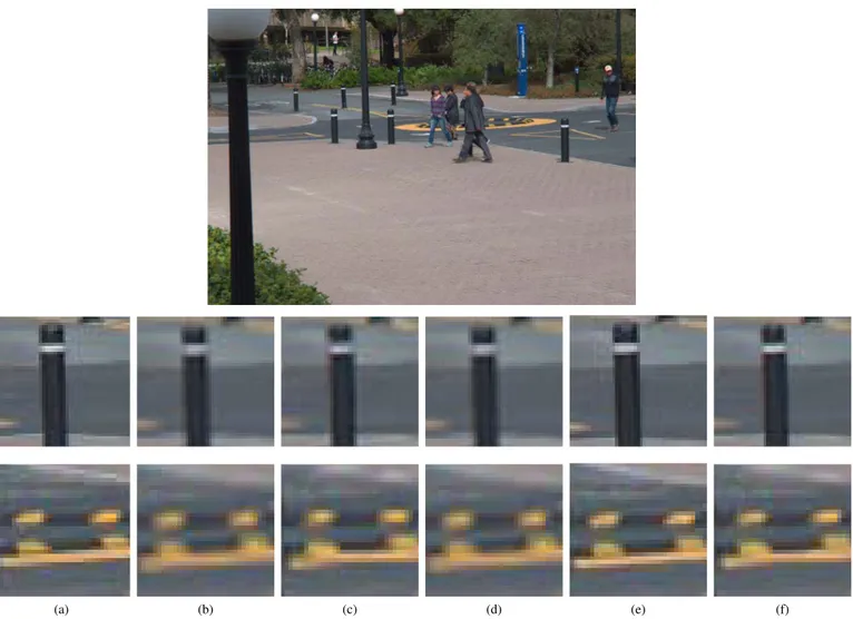
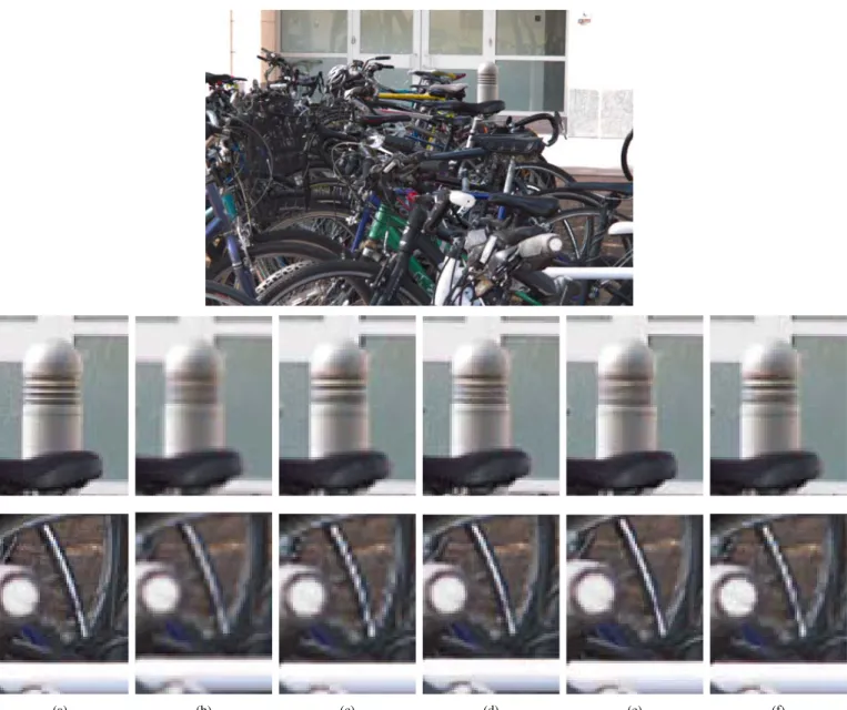
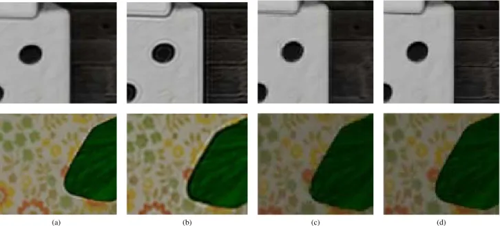
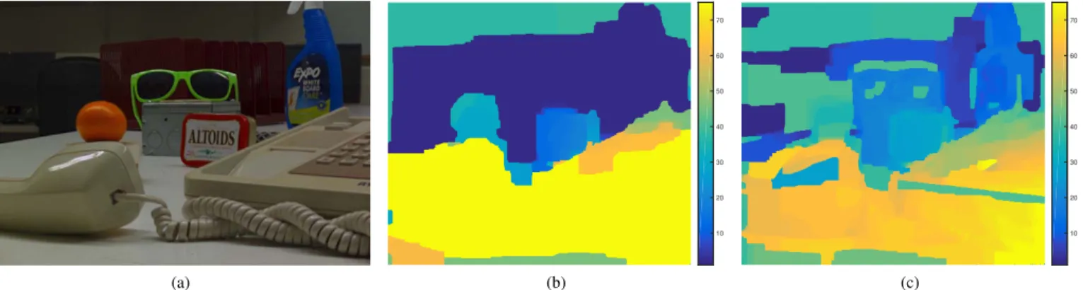
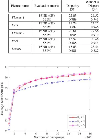
Spatial and angular resolution enhancement of light fields using convolutional neural networks
Tam metin
Şekil
Benzer Belgeler
The importance of angular correlations and the multipole mixing ratios has been shown previously (1-3); the experimental application of these vvere also discussed in
These computa- tions were based on a relativistic self constitent - field (Hartree - Fock - Slater) calculation to obtain the electron wave functions and the
A traffic is measured in erlangs which take into account the average duration of calls as well as their number, thus, if the average number of calls carried by a system in an hour
Keywords: Convolutional neural networks; mobilenet; keras; machine learning; deep learning, image classification tensor flow; python; skin cancer.6. iv
Key words: neural network, biometry of retina, recognition, retina based
Олардың сол сенімді орындауы үшін оларға үлкен жол көрсетуіміз керек, сондықтан біз химия пәнін агылшын тілінде байланыстыра оқыту арқылы
Hence, from the study by Luding [38], the authors considered that, during the increase in deviatoric stress, the particles in the shear band of the specimens tested under
Figure 2. A) At 26 weeks’ gestational age, sonogram revealed a thickened and confined placenta at the right uterine angle B) Subchorionic hematoma at the placental edge C)
