REGULAR ARTICLE
Balance in resource allocation problems: a changing
reference approach
Özlem Karsu1 · Hale Erkan2
Received: 6 March 2019 / Accepted: 5 February 2020 / Published online: 17 February 2020 © Springer-Verlag GmbH Germany, part of Springer Nature 2020
Abstract
Fairness is one of the primary concerns in resource allocation problems, especially in settings which are associated with public welfare. Using a total benefit-maximiz-ing approach may not be applicable while distributbenefit-maximiz-ing resources among entities, and hence we propose a novel structure for integrating balance into the allocation pro-cess. In the proposed approach, imbalance is defined and measured as the deviation from a reference distribution determined by the decision-maker. What is considered balanced by the decision-maker might change with respect to the level of total out-put distributed. To provide an allocation policy that is in line with this changing structure of balance, we allow the decision-maker to change her reference distribu-tion depending on the total amount of output (benefit). We illustrate our approach using a project portfolio selection problem. We formulate mixed integer mathemati-cal programming models for the problem with maximizing total benefit and mini-mizing imbalance objectives. The bi-objective models are solved with both the epsi-lon-constraint method and an interactive algorithm.
Keywords Bi-objective resource allocation problem · Fairness · Knapsack problem · Balance · Equity · Convex cones approach · Epsilon-constraint approach
1 Introduction
Allocating resources across multiple entities is a problem encountered in many real-life settings, hence resource allocation problems are widely studied in the opera-tional research (OR) literature (Luss 2012). Various decision support systems have
* Özlem Karsu
[email protected] Hale Erkan
1 Industrial Engineering Department, Bilkent University, Ankara, Turkey 2 McCombs School of Business, The University of Texas at Austin, Texas, USA
been proposed to help the decision-makers allocate resources so that the total output of the system is maximized.
Typically, resources are allocated so that the entities will enjoy benefits (out-puts), i.e., any resource allocation to entities is associated with an output alloca-tion. Resources and outputs can change based on the problem type: For example, in a healthcare resource allocation problem, resource can be budget and benefit can be measured with the number of people who benefit from a healthcare project or it can be measured by the quality adjusted life years1 (QALYs) gained by the
tar-get population. Even if in some situations where there could be projects which have some negative impacts (e.g., inadvertent adverse consequences due to treatments in healthcare projects), we assume that the projects generate a single output, and this represents benefits. Hence, throughout this paper, we use the terms output and ben-efit and also resource and input interchangeably.
The one widely used approach in resource allocation is total output maximiza-tion, also known as the utilitarian approach. This method focuses on maximizing the total output regardless of how it is distributed across the entities. It achieves the best result in terms of the total output; however, it may fail to sustain fairness (balance) in the allocation. This is because this approach may ignore allocating resources to entities that are not as good as the others at converting resources to output. Con-sider a healthcare project selection problem, where projects are categorized by target patients’ ages; resource usage is measured with the cost of a project and benefit is the resulting QALYs for a patient group. In this case, the utilitarian approach can result in a highly unfair resource distribution among categories. Elderly patients may not receive any resource, since these patient groups obtain relatively less benefit per unit resource devoted to them. Hence, using a utilitarian approach could be consid-ered a highly controversial decision.
One approach to ensure fairness can be equally dividing the resources among entities, if possible. However, such an allocation may also be inapplicable, since it may result in a high efficiency loss (sacrifice from the best level of the total output). In the same healthcare resource allocation problem, a policy maker may also find a completely equal resource allocation to infants and elderly unfair or unacceptable on the grounds that the society should provide more resources to younger generations. Between these two extremes (a total output maximizing allocation and fairness max-imizing allocation), there are other allocations, i.e., the problem is a bi-objective decision-making problem.
Moreover, as the example shows, fairness itself is a subjective concept, and hence it does not have a de facto definition. Depending on the problem setting and deci-sion-maker, several different criteria can be listed to describe a “fair” allocation. In this study, we suggest an approach that will accommodate these differences while incorporating balance concerns into the resource allocation process. The proposed method enables decision-makers to define a perfectly balanced allocation (reference allocation) differently at different levels of output. In order to achieve this structure,
1 QALY is a measure of health combining length and quality of life. It is widely used in studies focusing
a bi-objective mixed integer mathematical programming formulation is used. In addition, we engage both a posteriori and interactive solution approaches, which dif-fer in terms of decision-maker’s participation throughout the solution process.
In recent years, fairness has become an important criterion in many OR appli-cations. It is almost a mandatory criterion in decisions affecting social welfare as in public sector decision-making (see, e.g., (Butler and Williams 2002; Kelly et al. 1998; Smith et al. 2013; Mestre et al. 2012; Heitmann and Brüggemann 2014; Karsu and Morton 2015 and the references therein for a review of such applications).
Equity-related concerns can be categorized as equitability and balance (Karsu and Morton 2015). Equitability aims to achieve an even distribution of the resources or outputs, since it assumes that the entities are indistinguishable, i.e., the identities of the entities do not affect the decision. Balance concerns, however, are relevant in cases, where the entities have different characteristics. They may, for example, differ in terms of productivity, need or claims. In such cases, a completely equal allocation may be undesirable and the decision-maker may want to allocate the resource in dif-ferent proportions.
For the case where resource allocation across entities with different character-istics is considered, Karsu and Morton (2014) propose a bi-criteria framework to handle balance and total benefit maximization concerns. They suggest using a refer-ence distribution approach to measure how balanced a given distribution is. Simi-larly, Stewart (2016) uses a reference point approach to solve a real-life multi-objec-tive resource allocation problem where quantity, quality and balance are the main concerns.
In this paper, we follow this line of research and provide a methodology to help decision-makers to trade balance off against total benefit in resource allocation set-tings. We assume that the decision-maker has balance concerns for the output dis-tribution and extend the idea of balance measurement in Karsu and Morton (2014) to a piecewise linear concept, which allows the decision-maker to change her refer-ence proportion depending on the total output. The main contribution of this work in comparison with the previous work, especially the one by Karsu and Morton (2014), is the changing reference approach. This extension is a generalization of the previ-ous work and would provide more flexibility in real-life applications. This gener-alization significantly changes the structure of the bi-objective programming models solved, as will be discussed in Sect. 2.
The rest of the paper is as follows: In Sect. 2 we first introduce the imbalance measurement approach with changing reference proportions at different total output intervals. We exemplify the use of the approach on knapsack-type discrete resource allocation problems and provide the corresponding mathematical models. In Sect. 3, we discuss a further extension of the approach, which uses interpolation of threshold reference proportion vectors to assign a unique reference proportion vector to each total output value as opposed to using a fixed reference proportion for the whole interval. In Sect. 4, we demonstrate the feasibility of the approach by solving exam-ple problems using the epsilon-constraint method and providing the results of our computational experiments. For settings where the decision-maker (DM) is willing to provide preference information, we discuss an interactive approach and report on
its performance. We conclude the discussion in Sect. 5 by summarizing our results and pointing out some further research directions that could be pursued.
2 Problem definition
2.1 Changing reference proportions in resource allocation
We measure balance with respect to desired proportions of the decision-maker and allow her to change these proportions as the total output or the total input changes. In this section, we discuss this idea of changing reference proportions in detail.
The underlying idea is similar to that of the well-known allocation rule from Babylonian Talmud, which divides a given resource in different proportions, changing with respect to the total amount of resource and demand (see Young 1995 for a detailed description). The story is as follows: A man dies leaving a heritage and credits to three different creditors with amounts of 100, 200, and 300 units. According to Talmud’s rule, if the heritage is 100 units, each creditor gets 33.3 units (equal amounts); if heritage is 200 units then creditors receive 50, 75, 75 units, respectively, and if it is 300 units, they receive 50, 100, 150 units, respectively. In this allocation policy the received shares change depending on the total amount of heritage. When heritage is small, each creditor receives equal proportions; however, as the amount on hand increases their shares become pro-portional to their credits. If the decision-maker keeps the equal proportion policy in the third scenario, 100% of creditor one’s credits will be paid, while only 33.3% of creditor three’s credit will be covered. From creditor three’s perspective, this allocation may not be acceptable, and therefore in such situations, shifting the distribution from equal amounts may improve fairness.
A similar situation may also be seen in investment planning. Armbruster and Delage (2015) and Eeckhoudt and Schlesinger (2006) state that investors may become more risk tolerant when the potential output is higher. As the expected benefit gets higher, the investor becomes more prudent to invest in more risky projects, and hence the reference allocation changes.
We will explain the novel approach that we suggest for imbalance measure-ment in resource allocation settings using a small example as follows:
Assume that a local healthcare provider is planning the annual budget allot-ment for a set of proposed projects, each of which targets a different population group. For simplicity, consider a case with two population groups, which are sig-nificantly different with respect to their life styles. Let us assume that the first and second groups represent people who are negligent and cautious about their health, respectively. (Such behavioral differences could emerge due to other attributes of the groups such as income.) The provider measures health gain in terms of the total scores based on QALYs.
If the total score that would result from the allocation decisions is relatively low, the policy makers may prefer to use the resources such that benefit is evenly distributed across population groups. Making the allocation in favor of the group
that returns more benefit per unit resource (in our example this corresponds to the second group) would create a significant gap between their healthcare status; thus it may not be appropriate for ethical reasons. Conversely, if total score is relatively high (e.g., between 70 and 100), the overall community health may be consid-ered to be above standards. Since the overall health state is already good, having a more uneven distribution between population groups may be more acceptable. Both groups already have above satisfactory health status; hence, when benefit distribution shifts toward one of the groups, the difference would not be as strik-ing as the first case. Therefore the policy maker may prefer an allocation where the second population group has higher returns in order to increase total health score. To summarize, distributing a good in a fair manner may be more important when the total welfare is already low. As the total welfare increases, the allocator may want to shift resources to more productive entities.
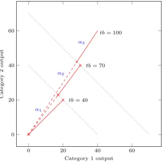
We illustrate the changing reference proportions in the example in Figure 1a, where there are two categories (population one and population two). The two axes represent the total benefit enjoyed by the categories, i.e., the total health score of each population. As long as the total benefit is below 40 units, decision-maker uses reference proportion 𝛼1 . This reference proportion is a vector showing the desired
benefit percentages for each group, in this example 𝛼1 = (0.5, 0.5) , i.e., if the total
benefit is below 40 units, the policy makers would like to distribute it evenly across the two groups. When the total benefit exceeds 40 units, he/she changes the refer-ence distribution vector from 𝛼1 to 𝛼2= (0.4, 0.6), and in this representation, he/she
prefers to see that the bigger portion of the benefit is in category 2. As the output increases, reference distribution becomes less even between categories.
This methodology can be applied to incorporate balance concerns in various resource allocation environments which can be formulated as: continuous knapsack problems, where benefits are obtained with respect to some production function,
dis-crete knapsack problems, where costs and benefit parameters are explicitly given,
or in assignment problems with capacity limitations. We illustrate the proposed approach using a discrete knapsack problem. Knapsack problem is a well-known combinatorial optimization problem, which has various real-life applications and is in the class of NP-hard problems (Kellerer et al. 2004). The problems that we for-mulate will trade balance off against total benefit, and hence they are bi-objective knapsack problems (see Carazo 2015 for a discussion on multi-criteria knapsack problems).
2.2 Mathematical model with interval‑based reference proportions
We consider a bi-objective discrete knapsack problem to illustrate our resource allo-cation mechanism. In the problem setting, suppose there are N proposed projects and each project incurs a cost of ci units and returns a benefit of bi units. Projects
are divided in different categories such that each project belongs to one (and only one) category. Let K be the number of categories and let K ≤ N . We assume that the decision-maker has a limited budget B, which is not enough to fund all of the
projects ( ∑N
i=1ci>B ). Benefit and cost values of each project are assumed to be
known, and hence productivity of each project is known a priori to the investments decision.
We define the binary variables 𝐱 = (x1, … , xN) as follows: xi= 1 if project i is
selected in the portfolio and 0 otherwise. We assume that the degree of imbalance
Fig. 1 Changing Reference Proportion Setting 0 20 40 60 0 20 40 60 α1 α2 α3 tb = 40 tb = 70 tb = 100 Category 1 output Cate gory 2o utpu t
aChanging reference proportions
0 20 40 60 0 20 40 60 real1 ref1 dev11 dev12 dev12 dev22 real2 ref2 Category 1 output Cate gory 2o utpu t
of any distribution is measured by its distance to a reference allocation, which dis-tributes the benefit according to DM’s desired (reference) proportions. We allow the DM to determine different reference proportions for different levels of total benefit distributed. Assume that there are M threshold values defining (M − 1) intervals (interval m is defined by threshold levels Tm and Tm+1 ). Reference proportion 𝛼mk
is the desired proportion of total benefit allocated to category k = 1, … , K if the total benefit is in interval m = 1, … , (M − 1) . Reference proportion can increase/ decrease as we move along on the intervals to shift the allocation in favor of particu-lar categories.
Recall our health benefit example with two population groups. Assume that the groups are constructed based on the individuals’ smoking habits (group 1: smok-ers and group 2: nonsmoksmok-ers). For simplicity, assume that there are two healthcare project portfolios: Portfolio 1 would result in 50 units of benefit to group 1 and 10 units of benefit to group 2 while Portfolio 2 provides 5 and 15 units to these two groups, respectively. Consider the reference proportions of (0.5, 0.5) when the total benefit is less than 40 and (0.4, 0.6) when it is more than 40 (for higher total benefit levels the DM would rather encourage the nonsmokers by allocating more benefit to that group). Then, at portfolio 1’s total benefit level, the DM would rather have (60*0.4, 60*0.6)=(24,36). We call this reference allocation and actual allocation of (50,10) the realized allocation. Similarly, at Portfolio 2’s total benefit level (20), the DM would rather distribute the benefit equally so its reference allocation vector is (20*0.5, 20*0.5)=(10,10) while the realized allocation is (5, 15).
Imbalance of a realized allocation is measured as the total component-wise deviation from reference distribution of that allocation. That would be (|50 − 24| + |10 − 36|) = 52 for Portfolio 1 and (|5 − 10| + |15 − 10|) = 10 for Portfolio 2. As seen, Portfolio 2 is more in line with the DM’s allocation preferences in terms of balance but it has less total benefit than the first one.
Figure 1b shows the component-wise deviations of two realized allocations from their reference allocation vectors. Realized allocations are represented with real1 , real2, and 𝐱1 , 𝐱2 are the corresponding decision variable vectors. These
two realized allocations have total benefits lying in different intervals, and their imbalance level will be calculated with respect to their own reference propor-tion vectors. By using the corresponding 𝛼 values, we calculate reference dis-tributions as follows; ref1
k= 𝛼1k ∑N i=1bix1i and ref 2 k= 𝛼2k ∑N i=1bix2i , k = 1, 2 .
Component-wise deviation from reference distribution can be measured as devjk=|realjk− refjk| j = 1, 2 k = 1, 2 . Then, imbalancej=∑Kk=1devjk j =1, 2.
Notations used throughout the paper for the mathematical formulations are intro-duced below: Problem parameters N: Number of projects K: Number of categories M: Number of thresholds B: Total budget ci: Cost of project i = 1, … , N
bi: Benefit of project i = 1, … , N
Tm: Threshold values defining intervals for total benefit values m = 1, … , M 𝛼mk: Reference (desired) proportion for category k in interval m
k =1, … , K m = 1, … , (M − 1) ( 𝛼m∈ RK , ∑ K k=1𝛼mk= 1) gik= { 1, if project 0, otherwise
TB: Total benefit of all the proposed projects ∑N i=1bi
𝛥Tm: Difference between two consecutive threshold values, Tm+1− Tm ,
m =1, … , (M − 1) Decision variables xi= { 1, if project i is accepted, i = 1, … , N 0, otherwise
Xm: Amount of benefit gained within the interval m = 1, … , (M − 1)
ym=
{ 1, if 0, otherwise
𝛼k: Selected reference proportion for each category k = 1, … , K ,
( ∑K
k=1𝛼k= 1)
Imbalance: Imbalance indicator of the benefit distribution
The proposed bi-objective interval-based reference proportion model (IRPM) is provided below: (1) max N ∑ i=1 bixi, min Imbalance (2) N ∑ i=1 cixi≤B (3) N ∑ i=1 bixi= (M−1)∑ m=1 Xm (4) X1≤𝛥T1 (5) Xm≥𝛥Tmym m =1, … , (M − 2) (6) Xm≤𝛥Tmym−1 m =2, … , (M − 1) (7) 𝛼k= 𝛼1k(1 − y1) + M−∑3 m=1 𝛼m+1k(ym− ym+1) + 𝛼M−1kyM−2 k =1, … , K
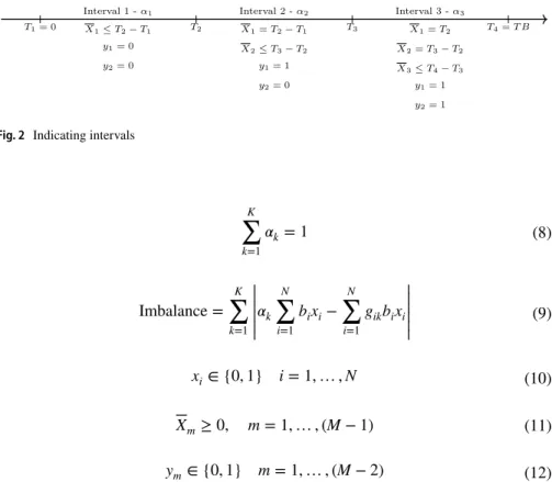
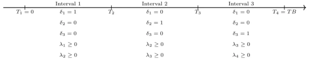
Constraint (2) ensures that the budget is not exceeded. Constraint (3) is used to cal-culate the total benefit of the projects which are selected in the portfolio. Constraints (4)–(6) are used to identify the interval of total benefit. If total benefit corresponds to interval m then {yj= 1 ∀j < m} and {yj= 0 ∀j ≥ m} . An example setting
with three intervals and four threshold points is presented in Fig. 2. Initial and last threshold values are set to the lower and upper bounds of total benefit value, respec-tively. In solutions where total benefit value ( ∑N
i=1bixi ) is smaller than T2 ; X1< 𝛥T1 ,
y1= y2= 0 and reference proportion vector 𝛼1 is used. When total benefit distrib-uted exceeds T2 , X1 is exactly equal to 𝛥T1 , y1 = 1 and reference proportion
vec-tor 𝛼2 is used. Lastly, if the solution has a total benefit value greater than T3 , then
both interval indicators; y1 and y2 take value 1, and reference proportion vector 𝛼3 is
assigned to the allocation.
The reference proportions change at the thresholds, and at each threshold, one of the two consecutive proportion vectors should be used. Without loss of generality, we assume that at each threshold Tm , 𝛼m will be used. If total
ben-efit can only have integer values, subtracting a small value, 0 < 𝜖 < 1 , from the threshold values restrains any solution from achieving a threshold value. If the total benefit does not necessarily have integer values, one can introduce binary variables to control whether total benefit distributed is equal to a threshold value and additional constraints to indicate which reference proportion vector should be assigned in such cases.
(8) K ∑ k=1 𝛼k= 1 (9) Imbalance = K ∑ k=1 || || ||𝛼k N ∑ i=1 bixi− N ∑ i=1 gikbixi|||| || (10) xi∈ {0, 1} i =1, … , N (11) Xm≥0, m =1, … , (M − 1) (12) ym∈ {0, 1} m =1, … , (M − 2) T1= 0 T2 T3 Interval 1 - α1 X1≤ T2− T1 y1= 0 y2= 0 Interval 2 - α2 X2≤ T3− T2 y1= 1 y2= 0 X1= T2− T1 Interval 3 - α3 X3≤ T4− T3 y1= 1 y2= 1 X1= T2 X2= T3− T2 T4= T B
Constraint (7) makes sure that 𝛼 is equal to the reference proportion vector of the corresponding interval. Imbalance is measured in (9), and it is calculated as the total deviation from the reference benefit distribution. The desired (reference) and actual benefits in category k are 𝛼k
∑N
i=1bixi and ∑ N
i=1gikbixi , respectively, for k = 1, … , K .
We add up the absolute difference between desired and realized benefits over all categories.
Constraint (9) involves nonlinear terms. We linearize them using additional auxil-iary variables: wki and dk . We delete constraint (9) and add the following:
Constraints (13)–(15) are used to linearize the product of 𝛼k (continuous) and xi
(binary) decision variables such that wki is equal to this product ( wki= 𝛼kxi).
With constraints (16)–(17) and the auxiliary variables dk , we rewrite the
abso-lute deviation value term with linear inequalities. New variable dk is the deviation
in category k from the reference distribution. This linearization works when dk s are
minimized in the objective function. If one has another model in which this is not the case, alternative linearization techniques should be used.
In the linearized model, there are 3KN + 2M + 2K + 2 constraints (excluding the set constraints) and N + 2M + 2K + NK − 2 variables, N + M − 2 of which are binary.
There is a well-known alternative approach to model such piecewise problems (Williams 2013). However, we use an incremental formulation that is computation-ally more efficient. We provide the alternative formulations and compare these for-mulations in terms of solution times in Appendix A. The results also justify our modeling choice.
In this formulation, each project is assumed to yield benefits that are relevant to one category only. The proposed approach can be easily extended for the more (13) wki≤xi k =1, … , K i =1, … , N (14) wki≤𝛼k k =1, … , K i =1, … , N (15) wki≥𝛼k− (1 − xi) k =1, … , K i =1, … , N (16) N ∑ i=1 biwki− N ∑ i=1 gikbixi≤dk k =1, … , K (17) N ∑ i=1 gikbixi− N ∑ i=1 biwki≤dk k =1, … , K (18) Imbalance =∑ k dk (19) wki≥0 k =1, … , K i =1, … , N
general case in which each project generates benefits in several categories. This is possible, for example, by apportioning the projects’ total benefits to different catego-ries by using fractional amounts. Such an extension could be built by relaxing the binary parameter gik such that gik∈ [0, 1] and ∑kgik= 1 , ∀i ∈ {1, … , N}.
3 Moving reference proportion model (MRPM)
In IRPM, there are multiple reference proportion vectors and the model assigns an
𝛼k based on the interval of the total benefit. The same reference distribution is used
for the entire interval between two thresholds, regardless of its distance from the threshold points. Although this may seem reasonable, in some cases, it may result in abrupt changes in the solutions, especially for the ones with total benefit closer to the thresholds.
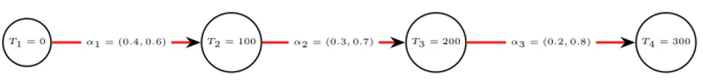
Let us consider the allocation policy in Fig. 3 with two categories. Until total benefit reaches T2= 100 units, 𝛼1 is (0.4, 0.6) and afterward it changes to (0.3, 0.7).
Suppose that there are two Pareto solutions with total benefit values 96 and 102 units. In the first solution, with 96 units of benefit, benefits are distributed as (38,58) units between categories. In the second solution, total benefit is in the second interval, and hence reference proportion vector shifts to (0.3,0.7) and benefit dis-tribution becomes (31,71) units. In the second solution, the benefit of category 1 decreases by 18% while benefit of category 2 increases by 22% . Even though total benefits are close to each other, these two distributions have significant differences. It may be expected that as the total benefit increases, each categories’ benefit will also increase; however, in the neighborhood of thresholds, results do not coincide with this expectation. For a fact, these increases/decreases are inevitable due to the selected reference distribution coefficients, while one category’s share is increas-ing, other’s have to decrease. Thus in the threshold neighborhoods, there are sudden jumps from one distribution to the other, which may be undesired.
In order to address this drawback, we enhanced our model to move 𝛼k values from
one threshold point to the other by using interpolation. For each total output value, the reference proportion vector is calculated uniquely by taking convex combination of two adjacent reference proportion vectors. This way, benefits of entities will grad-ually increase/decrease as the total benefit changes. In the previous example; where we have 96 units of benefit the corresponding reference proportion will be calcu-lated using equation 𝛼k= X1
(𝛼2k− 𝛼1k)
T2− T1 + 𝛼1k , in this example it is equal to (0.304,0.696). In the second solution, with 102 units of benefit, reference proportion
T1 = 0 α1 = (0.4, 0.6) T2 = 100 α2 = (0.3, 0.7) T3 = 200 α3 = (0.2, 0.8) T4 = 300
becomes (0.298,0.702). Consecutively, benefit distributions are (29,71) and (30,70), respectively. By moving the reference proportion vector from one threshold to the other, we can achieve a more moderate change in distributions.
We modify IRPM to formulate this change. Reference proportion constraint (7) is reformulated as below, and this adjusted model is referred as the moving reference proportion model (MRPM).
This term is nonlinear due to the product of variables ym (binary) and Xm
(continu-ous). We linearize it with the additional decision variable tmm, and the new
formu-lation contains the constraints of the IRPM models except constraint (7) with the following: 𝛼k= (1 − y1) [X 1(𝛼2k− 𝛼1k) 𝛥T1 + 𝛼1k ] + M−∑2 m=2 (ym−1− ym) [X m(𝛼m+1k− 𝛼mk) 𝛥Tm + 𝛼mk ] + yM−2𝛼M−1k k =1, … , K (20) 𝛼k= [ X1(𝛼2k− 𝛼1k) 𝛥T1 + 𝛼1k ] − [ t11(𝛼2k− 𝛼1k) 𝛥T1 + y1𝛼1k ] + M−∑2 m=2 [(t m−1m(𝛼m+1k− 𝛼mk) 𝛥Tm + ym−1𝛼mk ) − ( tmm(𝛼m+1k− 𝛼mk) 𝛥Tm + ym𝛼mk )] + yM−2𝛼M−1k k =1, … , K (21) tmm≤X UB m ym m =1, … , (M − 2) (22) tmm≤Xm m =1, … , (M − 2) (23) Xm− XUBm (1 − ym) ≤ tmm m =1, … , (M − 2) (24) tm−1m≤XUBm ym−1 m =2, … , (M − 2) (25) tm−1m≤Xm m =2, … , (M − 2) (26) Xm− XUBm (1 − ym−1) ≤ tm−1m m =2, … , (M − 2) (27) tmm≥0 m =1, … , (M − 2)
In linearization, upper and lower bounds on Xm are set to 𝛥Tm and 0, respectively
(The upper bound is denoted as XUBm ). This model has 3KN + 8M + 2K − 13
con-straints and N + 4M + 2K + NK − 7 decision variables.
It is possible to make improvements to the formulations by introducing sim-ple valid inequalities. Recall the binary variable ym , which is used as the interval
indicator as follows: When total benefit is in interval m, {yj= 1 ∀j < m} and {
yj= 0 ∀j ≥ m} . Hence, whenever ym= 1, we have yj= 1∀j ≤ m − 1 and we
tighten the models by adding the following constraints:
Models IRP and MRP represent the general formulation of the proposed bi-objective resource allocation problem. We conducted preliminary experiments to analyze the effect of improvements suggested. We have observed that the percentage improve-ment in solution time is positive in most instances, and hence we use the model vari-ants with these improvements in our main experiments for both IRPM and MRPM. From now on, IRPM and MRPM will refer to their variants with the improvements.
In Appendix A, we provide alternative formulations for this problem as discussed before and show that the formulation we suggest outperforms these alternative for-mulations in most instances.
4 Computational experiments
4.1 An illustrative example
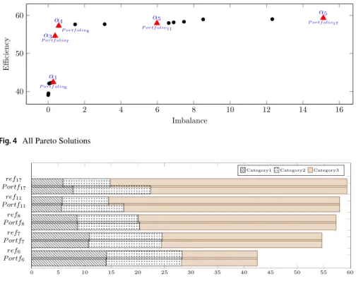
As an example, we solve IRPM for a real-life R&D project selection problem of a public sector agency, where the projects belong one of the three sector-based cat-egories (this problem is considered from an input-oriented aspect and with a single reference allocation in Karsu and Morton 2014). There are 39 projects, whose cost and benefit (output) values are assumed to be known. The budget is taken as 45% of the total cost of all the projects available. We determine four thresholds and solve the bi-objective problem using the epsilon-constraint approach (see Appendix B for a pseudocode of the approach). In the example, without loss of generality, it is assumed that as total benefit distributed increases DM prefers more uneven distribu-tions that encourage more productive categories (Category 3). Figure 4 shows the set of all nondominated solutions, and Fig. 5 shows the realized and the reference benefit distributions of five example solutions.
Figure 4 shows some example portfolios from different parts of the frontier and the 𝛼 vectors used to assess imbalance for these portfolios. In Fig. 5 we also see how the output would be distributed if it were possible to realize the desired proportions. On the left hand side of the Pareto front, we have an example bal-anced allocation, Portfolio6 , with 42.45 units of total benefit which uses reference
(28)
tm−1m≥0 m =2, … , (M − 2)
(29)
proportion vector 𝛼 = 𝛼1= (0.33, 0.33, 0.33) . This solution ensures an even
ben-efit allocation across the three categories, as desired. Two solutions in the mid-dle, Portfolio7 and Portfolio8 have higher total benefit than Portfolio6 . The realized
distributions in these portfolios slightly deviate from their reference distributions, but they are still close. Portfolio11 is another example that has higher total benefit
than the previous portfolios. On the other extreme, there is the total benefit-max-imizing solution, Portfolio17 , with 59.32 units of benefit and a higher imbalance
value. In this portfolio, one can see that the realized distribution notably deviates from the reference. However, it is the best solution given this total benefit level since the model ensures that for any total benefit level, a maximally balanced solution is returned. As we move toward the maximum total benefit extreme, out-puts of category 3 are significantly higher than those of the first two categories in the reference distributions and hence in the realized distributions. By present-ing such Pareto solutions, we allow DMs to extensively understand the trade-off between the total benefit maximizing and most balanced solutions and to which extent their desired (reference) allocations can be realized in each interval. The DM can choose from the given set of alternatives based on her preferences. More-over, such visualizations help to structure discussions and negotiations between different parties that might be affected by allocation decisions.
Throughout the paper, we make the analysis assuming that DM encourages more productive categories in higher output levels. However, it is also possible to
0 2 4 6 8 10 12 14 16 40 50 60 α3 α4 α5 α1 P ortf olio6 P ortf olio7
P ortf olio8 P ortf olio11
α5
P ortf olio17
Imbalance
Efficiency
Fig. 4 All Pareto Solutions
0 5 10 15 20 25 30 35 40 45 50 55 60 ref6 P ortf6 ref7 P ortf7 ref8 P ortf8 ref11 P ortf11 ref17 P ortf17
Category1 Category2 Category3
implement a reversed policy meaning that, in certain problem settings, DM may pre-fer more even distributions when total benefit is higher. Such a change in the policy would not require any adjustments in the model other than changing 𝛼mk parameters.
4.2 Data generation
In this part, we discuss the computational experiments that we performed to demon-strate the feasibility of the approach. We generated problem instances and engaged the epsilon-constraint method to solve the resulting bi-objective programming prob-lems. We first discuss the details of our data generation scheme and then report the results of our computational tests.
In different decision-making environments, parameters may have certain charac-teristics; for instance, relation between cost and benefit values can vary or produc-tivity of projects may differ depending on the category of each project. In order to reflect special properties of different problem settings we performed computational experiments on different problem instances.
In order to mimic different types of project portfolio selection problems that could be encountered in real life and to analyze the effect of parameters on solution times, we considered three different problem types. In all problem types, cost values have discrete uniform distribution with integer parameters 1 and R, R ∈ {30, 100} , ( ci∼ discrete uniform (1, R) i = 1, … , N ). Benefit values are generated with a
differ-ent policy in each problem type. In type A instances, benefit is generated randomly, while in types B and C, it is generated using a linear function of cost. Problem types are described below.
Uncorrelated Instances (Type A): Benefit values are also randomly distributed between [5, R], i.e. bi∼ discrete uniform (5, R) i = 1, … , N . In this type, there is
no correlation between cost and benefit values, i.e., productivity of the projects are randomly determined.
Strongly Correlated Instances (Type B): In this type, benefit values are positively correlated with the cost values. bi= tci+ a i =1, … , N where t ∈ ℝ+ and a ∼
dis-crete uniform (0, R/10). t is an indicator of productivity and a is used to have some diversity among projects. In our experiments, we set t as 1.2.
Category-Based Strongly Correlated Instances (Type C): In this type, each category has a different level of productivity, and hence tk is used instead of t.
bi=∑Kk=
1giktkci+ a i =1, … , N (Recall that gik is 1 if project i belongs to
cat-egory k and 0 otherwise). In our experiments we set t1= 1.2 , t2= 1.5 , t3= 1.8 when
K =3 and additionally t4= 2.0 when K = 4.
In all of the generated instances budget, B, is set to ⌊ ∑N
i=1ci
2 ⌋ . We generated prob-lem instances with 3 and 4 categories and assumed there are 5 intervals defined by 6 threshold points. The threshold levels defining the intervals are determined as a function of TB = ∑N
i=1bi . The 𝛼m and T values are provided in Table 1. The
thresh-old levels and 𝛼m values used are for illustrative purposes. In real life, other levels
The algorithms are coded in Java and the computational studies are performed on Eclipse. All mathematical models are solved using CPLEX 12.8. All of the instances are solved in a computer with Intel Xeon CPU E5-1650 3.6 GHz processor and 32 GB RAM. Computation times are given in central processing unit seconds (CPU). 4.3 Epsilon‑constraint method results
We first used the epsilon-constraint method (Haimes et al. 1971) to find the set of nondominated solutions (A solution is nondominated if it is not possible to find another solution which is at least as good as it with respect to both total benefit and balance). Starting from the nondominated solution that has the minimum imbalance value, in each iteration it finds a new solution by minimizing imbalance and restrict-ing total benefit by a constraint. In each iteration, two srestrict-ingle objective models are solved ( min imbalance and max ∑N
i=1bixi ) to ensure that a nondominated solution
is found. At each iteration, the solution of the first model is feasible for the second model, which maximizes total benefit fixing the imbalance to the value found in the first one. We use this solution as an initial solution to the second model. Moreover, some of the interval-defining variables ( yms ) can be fixed since the total benefit in
the second model will be at least as much as the total benefit found by solving the first model.
Similarly, in the models where the total benefit level is restricted via an epsilon-constraint, some information on potential intervals is also available, e.g. some of the lower intervals are not possible anymore. Therefore, we fix the values of several variables in the model that are used to select the interval (see the algorithm descrip-tion in Appendix B). We performed our main computational experiments exploiting this problem specific property when using the epsilon-constraint method.
Any algorithm that is designed for bi-objective integer programming problems can be used to find the set of nondominated points (see, e.g., Chalmet et al. 1986; Ralphs et al. 2006 for algorithms based on weighted sum and Tchebycheff scalariza-tions, respectively. See also Boland et al. 2015 for a recent solution algorithm and the references therein for further examples.)
Details of the epsilon-constraint algorithm are provided in Appendix B. All benefit parameters are integer in our problem instances, therefore it is possible to
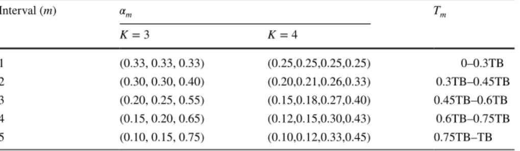
Table 1 Reference 𝛼m and corresponding T values
Interval (m) 𝛼m Tm K = 3 K = 4 1 (0.33, 0.33, 0.33) (0.25,0.25,0.25,0.25) 0–0.3TB 2 (0.30, 0.30, 0.40) (0.20,0.21,0.26,0.33) 0.3TB–0.45TB 3 (0.20, 0.25, 0.55) (0.15,0.18,0.27,0.40) 0.45TB–0.6TB 4 (0.15, 0.20, 0.65) (0.12,0.15,0.30,0.43) 0.6TB–0.75TB 5 (0.10, 0.15, 0.75) (0.10,0.12,0.33,0.45) 0.75TB–TB
generate the whole set of nondominated solutions. Presenting the set of all nondomi-nated solutions is useful for the DM to see the trade-off between the two criteria considered. It informs the DM on the effect of changing the portfolio from one effi-cient solution to the other.
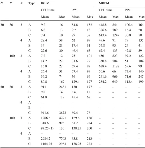
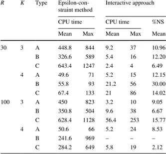
We solve five instances for each problem type, N, K and R combinations, and report the average and maximum values of the solution time and number of exact nondominated solutions obtained, |NS|, for the IRP and MRP models, respectively.
Results of the IRPM and MRPM are provided in Table 2. We use a time limit of 3 h as follows: If an instance cannot be solved within 3 h, that is, if the whole set of Pareto solutions cannot be returned, we terminate that instance and its values are not included in the performance metrics. Number of instances that cannot be completed within the time limit is reported in parenthesis in the column reporting the average CPU time. If, for a set of instances, at least 3 out of 5 instances could not be solved
Table 2 IRP and MRP model results
N R K Type IRPM MRPM
CPU time |NS| CPU time |NS|
Mean Max Mean Max Mean Max Mean Max
30 30 3 A 9.2 16 84.8 152 448.8 844 100.4 164 B 6.8 13 9.2 13 326.6 589 16.4 20 C 7.4 10 29 37 643.4 1247 30.8 50 4 A 28.4 58 62 99 49.6 71 79 135 B 14 21 17.4 31 55.8 93 24 41 C 22.6 30 46.4 65 67.4 133 42.8 59 100 3 A 7.2 12 75 101 450 823 97.2 122 B 14.2 22 31.6 79 350.8 504 51 104 C 15.8 22 59.4 97 628.4 1128 59.6 99 4 A 26.4 51 57.4 99 50.6 66 77.4 140 B 36.2 74 36 66 241.6 969 71.6 247 C 80.8 169 129.4 197 284.2 649 113.4 199 50 30 3 A 911 2431 130 177 – – – – B 9.8 14 8.6 12 – – – – C 61.8 128 45.4 68 – – – – 4 A – – – – – – – – B – – – – – – – – C 941.6 3672 69.4 76 – – – – 100 3 A 1266.8 4291 129.6 188 – – – – B 318.6 993 61.2 224 – – – – C 97.25 (1) 120 138.25 200 – – – – 4 A – – – – – – – – B 2984.2 7703 63.8 213 – – – – C 1164.25 2983 178.25 223 – – – –
within the time limit, we do not report the results of the set. Such cases are indicated with “-” in the table.
Due to the additional constraints and binary variables, MRPM’s solution times are significantly higher than IRPM. |NS| values also tend to increase in this approach, with exceptions in Type C problems. None of the larger MRPM instances with N = 50 could be solved within the time limit, and hence we do not provide results for these cases.
Type A problem instances lead to relatively larger solution sets, making the total solution time higher than the other types in most cases. On the other hand, Type B problems have the least number of nondominated solutions, indicating a rela-tion between the correlarela-tion structure and the number of nondominated solurela-tions obtained.
There are two factors that affect the total computational time: the number of nondominated points ( |NS| ), which dictates the number of single objective mod-els solved in the algorithm, and the time required for solving each single objective model. Knapsack problems’ solution times highly depend on the characteristic of parameter set. Some parameter sets are observed to be harder to solve. Pisinger (2005) analyses the performance of different algorithms on a variety of randomly generated knapsack problem instances, which differ in terms of the correlation between cost and benefit values of projects. He concludes that the easiest problem instances usually have uncorrelated benefit and cost values and the hardest prob-lem instances have strongly correlated benefit and cost values. Our observations are in line with these conclusions: the time required per model is smallest in Type A instances and highest in Type B instances. Again, this seems to be because in Type B problems, cost and benefit values are correlated with a constant parameter t. When we set t category-specific as in Type C instances, we change the correlation structure between cost and benefit and obtain an intermediate setting between the two extremes of Type A (uncorrelated) and Type B (strongly correlated) instances. With a few exceptions, the number of nondominated solutions and time per model nondominated solution (time per single objective model) of Type C instances are between those of Type A and Type B instances.
Increasing the problem size (N) makes the corresponding problems significantly more difficult to solve, as expected. Increasing the number of categories (K) how-ever has opposite effects in IRPM and MRPM. The MRPM becomes easier to solve when the number of categories is increased from 3 to 4, ceteris paribus. Moreover, it is observed that problems with a higher range parameter (R) tend to have larger Pareto sets and higher solution times.
4.4 Interactive approach
In the epsilon-constraint method, two models are solved to find each nondomi-nated solution and many instances cannot be solved in reasonable time due to the high number of iterations required and rapidly increasing solution times. One way of handling this challenge is using metaheuristic algorithms that return a set of
approximate Pareto solutions. Such algorithms are computationally very efficient; however, the solutions are neither exact nor with a quality guarantee.
Whenever possible, one can use preference information from the DM and focus only on nondominated solutions that could be of interest to him/her. We now discuss such an interactive approach that could be used to guide the DM to his/her most pre-ferred solution, without generating all the nondominated solutions beforehand. This approach requires less time as it does not generate the nondominated solutions that would not be of interest to the DM. It also helps the DM by guiding him/her to the most preferred solution as opposed to just presenting him/her the set of nondomi-nated solutions, which may be too large.
The interactive algorithm we use is based on the approach proposed in Lokman et al. (2016) to find the most preferred alternative of a DM for multi-objective inte-ger programming settings. We adjust this method to our bi-objective mixed inteinte-ger programming problems.
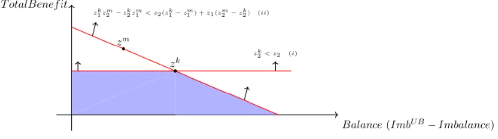
The fundamental assumption of the algorithm is that the DM has a non-decreas-ing quasiconcave utility function, which is unknown. Given this assumption and preference information from the DM (mostly in terms of pairwise comparisons of alternative solutions), one can infer that some parts of the feasible criteria space would not contain the most preferred solution and hence can eliminate them from further consideration. The method is called the convex cone method and such areas are called (convex) cone-dominated areas (Korhonen et al. 1984).
The algorithm keeps an incumbent, which is the most preferred nondominated solution so far. At each iteration, a challenger is generated for the incumbent by solving scalarization model (a weighted sum model) and preference information between a new pair of solutions is obtained from the DM. Let zm and zk be such two
nondominated solutions in the Pareto front. Then either zm≻zk or zk≻zm , where
≻ denotes the binary relation “is preferred to”. Given this pairwise comparison, a
2-point cone is defined as follows: C(zm, zk) ={z ∶ z = zk+ 𝜇(zk− zm), 𝜇 ≥ 0}
if zm⪰ zk . Korhonen et al. (1984) prove that if the DM has a quasiconcave utility
function, a point in the cone cannot be better than the cone generators, which are
zm and zk , in our example. Moreover, the corresponding cone-dominated region
CD(zm, zk) ={z�∶ z�≤zfor some z ∈ C(zm, zk)} (assuming both objectives are of
a maximization type) cannot contain the most preferred solution for the DM and hence is eliminated from the criterion space. When there are multiple such pairwise comparisons, all the corresponding cone-dominated regions are eliminated. These steps are repeated until the most preferred solution is the only feasible solution to the problem. For the sake of simplicity, we formulate the problem such that both objectives are of maximization type by defining Balance = ImbUB− Imbalance ,
where ImbUB is an upper bound on imbalance. Let z
1(x) be the balance value of a
solution x and z2(x) be the total benefit value of a solution x (both to be maximized).
Figure 6 demonstrates a two-point cone and the corresponding cone-dominated region for our bi-objective problems. Assuming zm≻zk and zm
2 >z k 2 , it directly fol-lows that zm 1 <z k 1 (since z
k is nondominated). As shown by Lokman et al. (2016),
any point z that is not cone-dominated has to satisfy at least one of the conditions (i), (ii), as otherwise it is in the cone-dominated region (shaded). The algorithm guarantees that a newly found nondominated solution is not dominated by any of the
cones generated so far, by using binary variables in the scalarization model. These variables enforce any new nondominated solution found by the scalarization model to satisfy at least one of the two conditions (i) and (ii). The pseudocode of the algo-rithm is provided in Appendix B.
We re-solved the problem instances with the interactive algorithm, using a quad-ratic function to represent DM’s underlying utility function, max ∑2
i=1−w 2
i(z I i− zi)2
where w = (0.7, 0.3) and zI denotes the ideal point z I
i = maxx∈Xzi(x), i = 1, 2 . This
utility function is only used to simulate the answers of the DM to the pairwise com-parison questions asked by the algorithm. The algorithm would work for any DM whose preference model is in line with a quasiconcave utility function. The most preferred solution and the performance of the interactive algorithm, in terms of the number of questions asked, is expected to change as the underlying preference model changes.
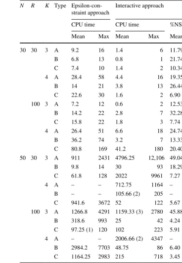
The results of these experiments are summarized in Tables 3 and 4. Instead of |NS|, we report the average values for the percentage of nondominated solutions found until determining the most preferred alternative. This percentage is calculated as follows:
The number of solutions found is equal to the number of pairwise questions asked to the DM. Compared to the epsilon-constraint approach, in most of the cases this approach solves the problems in considerably less CPU time and number of itera-tions. This effect is even more prominent in Type C problems, where only a small portion of the set of nondominated solutions needs to be generated before identify-ing the most preferred solution. There are, however, exceptions to this observation: for example, for IRPM, in most problems with N = 50 , the interactive algorithm requires more time than the epsilon-constraint approach. A similar situation occurs in MRPM for Type B instances with R = 100, K = 4 . This may be due to the extra constraints preventing any newly found solution to be cone-dominated, making the models harder to solve.
We observe the effect of problem size in the performance of the interactive algo-rithm, too. As N increases, the solution time increases, making some of the problems
%NS = Number of solutions found in the interactive algorithm
|NS| × 100
Balance (ImbU B− Imbalance) T otalBenef it
zk zm
zk2 < z2 (i)
zk1 z2 − zm 2 zk1 < z2(zm 1 − zk m1 ) + z1(zm2 − zk2 ) (ii)
unsolvable within the time limit of 3 h. “-” sign indicates that 3 out of 5 instances could not be solved within the time limit. Nevertheless, the interactive algorithm is able to solve more of the problem instances that could not be solved using the epsilon-constraint approach. This shows the value of using preference information, whenever possible.
5 Conclusion
We consider resource allocation problems, in which an indivisible resource is allocated across multiple entities so that they will enjoy benefits. Motivated by the fact that a pure total benefit-maximizing approach may not be appropri-ate in terms of balance, we suggest a bi-objective framework that trades balance
Table 3 IRPM-interactive approach performance comparison
N R K Type
Epsilon-con-straint approach Interactive approach
CPU time CPU time %NS
Mean Max Mean Max Mean
30 30 3 A 9.2 16 1.4 6 11.79 B 6.8 13 0.8 1 21.74 C 7.4 10 1.4 2 10.34 4 A 28.4 58 4.4 16 19.35 B 14 21 3.8 13 26.44 C 22.6 30 1.6 2 6.90 100 3 A 7.2 12 0.6 2 12.53 B 14.2 22 2.8 7 32.28 C 15.8 22 1.8 3 7.74 4 A 26.4 51 6.6 18 24.74 B 36.2 74 3.2 7 13.33 C 80.8 169 41.2 180 20.40 50 30 3 A 911 2431 4796.25 12,106 49.04 B 9.8 14 30 93 18.29 C 61.8 128 2022 9961 7.27 4 A – – 712.75 1164 – B – – 105.66 (2) 205 – C 941.6 3672 52 122 5.67 100 3 A 1266.8 4291 1159.33 (3) 2780 45.88 B 318.6 993 25 42 4.24 C 97.25 (1) 120 102 223 5.91 4 A – – 2006.66 (2) 4347 – B 2984.2 7703 48.75 86 6.40 C 1164.25 2983 215 718 3.45
off against total benefit. We capture the cases where the decision-maker’s under-standing of balance changes as the total amount distributed changes. We exem-plify the proposed method on project portfolio selection problems, where the pro-jects belong to different categories and there is a concern for ensuring a balanced allocation of the benefit as well as maximizing total benefit. We solve the result-ing bi-objective optimization problems usresult-ing the epsilon-constraint method and also implement an interactive algorithm that finds the most preferred solution of a DM.
In real-life decision-making settings, some pragmatic challenges may be encoun-tered in implementing the approach. We list some of these and potential ways to address these challenges: The proposed recommendation depends on the threshold levels. If these are not already available, they can be defined as a function of some problem dependent parameter (such as proportions of total benefit of the considered projects as we did in the computational experiments or proportions of the maximum attainable total benefit). If specific threshold values are difficult to obtain, one can perform sensitivity analysis by solving the problem multiple times, each time with a different choice of these parameters. One can then determine the winner portfo-lios in the sense that they are nondominated in most scenarios (different choices of parameters).
In some real-life problems arising in public domain, the benefits can be hard to ascertain in ways that are incontestable (given that there may be a need to make scoping choices concerning direct vs. indirect benefits, or benefits which are real-ized in the short vs. long term); thus, the elicitation of reference proportions could prove challenging in practice. Some of these challenges can still be addressed using the same structure by extending the problem dimensions. When multiple types of
Table 4 MRPM-interactive approach performance comparison, N = 30
R K Type
Epsilon-con-straint method Interactive approach
CPU time CPU time %NS
Mean Max Mean Max Mean
30 3 A 448.8 844 9.2 37 10.96 B 326.6 589 5.4 16 12.20 C 643.4 1247 2.4 4 6.49 4 A 49.6 71 5.2 15 12.15 B 55.8 93 21.2 56 30.00 C 67.4 133 21 86 14.02 100 3 A 450 823 3.2 10 9.05 B 350.8 504 9.6 38 6.67 C 628.4 1128 56.4 253 15.77 4 A 50.6 66 5.2 24 8.53 B 241.6 969 – – – C 284.2 649 5.8 19 2.12
quantifiable benefits exist (such as long term versus short term benefits), a multi-objective programming extension of the structure could be used, showing the trade-off between total benefit and balance in the allocations of multiple benefits. This would, of course, make the mathematical models more difficult to solve. In a prob-lem where there are p benefits (e.g. short term and long term), the resulting models will have 2p objective functions.
In this study, we suggested formulations and solution approaches for a setting where balance on the output distribution is sought. Balance could also be defined with respect to the resource devoted to the entities. Although it is very relevant and desirable to define balance with respect to the input in some settings, in some oth-ers it may not provide an agreeable solution. Especially in cases where the entities’ productivities (i.e., their ability to convert resources to outputs) are very different, indirectly controlling the output allocation by managing the resource allocation may not be straightforward. However, whether one should ensure balance in the resource allocation or output allocation is context-specific. Observing and reporting on the difference between these two approaches is an interesting direction for future research and applications.
Considering balance concerns explicitly in the decision support systems will provide useful insights to the decision-makers on the alternative allocation options and the trade-off between total benefit and balance concerns. Further research can be performed on the multi-objective version of the problem, in which relationship among different balance and efficiency measures can be examined.
Acknowledgements This study was supported by TUBITAK (The Scientific and Technological Research Council of Turkey) under Grant Number: 215M713. We thank the anonymous reviewers for their thor-ough feedback and constructive comments, which led to substantial improvement of the manuscript. Appendix A: Alternative formulations
Recall the alternative formulations mentioned in Sect. 2.2. These are provided in this section.
IRP alternative formulations
For IRP, alternative formulation 1 is a standard formulation that writes any total ben-efit value as a convex combination of the threshold values with the help of continuous variables ( 𝜆 ) showing these coefficients and a binary variable vector 𝛿 indicating the interval that the total benefit value belongs to. Alternative formulation 2 is similar to Alternative 1 but without the 𝜆 variables. Finally, we provide alternative formulation 3, which is similar to the proposed variant, but handles the interval fixing variables ( ym s)
IRPM alternative formulation 1
Figure 7 shows how the decision variables are set in these formulations.
IRPM alternative formulation 2: This formulation is the similar to Alternative 1 but without the 𝜆 variables.
(30) max N ∑ i=1 bixi, min Imbalance (2), (8), (10), (13) − (19) N ∑ i=1 bixi= M ∑ m=1 𝜆mTm (31) 𝜆1 ≤𝛿1 (32) 𝜆m≤𝛿m−1+ 𝛿m m =2, … , M − 1 (33) 𝜆M≤𝛿M−1 (34) M−∑1 m=1 𝛿m= 1 (35) M ∑ m=1 𝜆m= 1 (36) 𝛼k= M−∑1 m=1 𝛿m𝛼mk ∀k ∈ K (37) 𝛿m∈ {0, 1} m =1, … , (M − 1) (38) 0 ≤ 𝜆m≤1 m =1, … , M T1= 0 T2 T3 T4= T B Interval 1 δ1= 1 δ2= 0 δ3= 0 λ1≥ 0 λ2≥ 0 Interval 2 δ1= 0 δ2= 1 δ3= 0 λ2≥ 0 λ3≥ 0 Interval 3 δ1= 0 δ2= 0 δ3= 1 λ3≥ 0 λ4≥ 0
IRPM alternative formulation 3: This formulation is a variant of the proposed formulation, where the ym variables are set differently. We replace constraints
(3)–(6) and 11 in the proposed formulation with constraints (41) and (42) and obtain the following model:
where BigM = maxm{Tm+1, TB − Tm+1}.
MRP alternative formulations MRPM alternative formulation 1
MRP alternative formulation 1 is the modified version of Alternative 1 for the IRPM, for the moving reference case. For MRP, 𝛼 is also a convex combination of threshold proportions. Hence the same coefficient variables ( 𝜆 ) are used to deter-mine 𝛼 . Alternatives 2 and 3 are the modified versions of IRP Alternatives 2 and 3 for the moving reference setting, respectively.
(39) max N ∑ i=1 bixi, min Imbalance (2), (8), (10), (13) − (19), (34), (36), (37) M−∑1 m=1 𝛿mTm≤ N ∑ i=1 bixi (40) N ∑ i=1 bixi≤ M−∑1 m=1 𝛿mTm+1 (41) max N � i=1 bixi, min Imbalance (2), (7), (8), (10), (12) − (19) ym≤1 −Tm+1− ∑N i=1bixi BigM m =1, … , (M − 2) (42) ∑N i=1bixi− Tm+1 BigM ≤ym m =1, … , (M − 2)
MRPM alternative formulation 2
To linearize the multiplication: Define new continuous variables: hmi= 𝛿m× xi for
all m = 1, … , M − 2 and i = 1, … , N . Add the following constraints:
MRPM Alternative Formulation 3
Tables 5 and 6 show the comparisons of alternative formulations in terms of average and maximum solution times, for IRP and MRP models, respectively. In Table 5, it is observed that all formulations have very close solution times for smaller instances of IRP. As the problems get larger, the proposed formulation performs notably better in most settings but there is no clear winner. For N = 50 , R = 100 , K = 4 instances, the alternative formulations failed to return solutions to some of the type B and C instances, while with the proposed formulation it was possible to solve them within the time limit. It is also clearly seen in Table 6 that alternative formulations 1 and 2 perform significantly worse than MRPM. The performances of MRPM and alterna-tive 3, which is actually quite similar to MRPM, are comparable.
(43) max N ∑ i=1 bixi, min Imbalance (2), (8), (10), (13) − (19), (30) − (35), (37), (38) 𝛼k= M−∑1 m=1 (𝜆m𝛼mk) + 𝜆M𝛼M−1k ∀k = 1, … , K max N � i=1 bixi, min Imbalance (2), (8), (10), (13) − (19), (34), (37), (39), (40) 𝛼k= M−�2 m=1 𝛿m �(∑ ibixi− Tm)(𝛼m+1k− 𝛼mk) 𝛥Tm + 𝛼mk � + 𝛿M−1𝛼M−1k ∀k ∈ K (44) hmi≥xi+ 𝛿m− 1 m =1, … , M − 2, i = 1, … , N (45) hmi≤𝛿m m =1, … , M − 2, i = 1, … , N (46) hmi≤xi m =1, … , M − 2, i = 1, … , N (47) hmi≥0 m =1, … , M − 2, i = 1, … , N max N ∑ i=1 bixi, min Imbalance (2), (8), (10), (12) − (28), (41), (42)
Appendix B: Solution methods
We used the well-known epsilon-constraint method to obtain exact Pareto front. Additionally, we used an interactive approach to find the most preferred solution. Both methods are provided below.
Let the generic model be:
where x and X denote the decision variable vector and the feasible region, respectively.
min Imbalance, max
N
∑
i=1
bixi x ∈ X
Table 5 CPU time comparison among alternative IRP models
N R K Type IRPM Alternative 1 Alternative 2 Alternative 3
Mean Max Mean Max Mean Max Mean Max
30 30 3 A 9.2 16 9.75 21 8.8 16 8.6 19 B 6.8 13 5 8 4.8 7 7.4 17 C 7.4 10 7.75 11 7.2 10 7.4 10 4 A 28.4 58 25.5 37 25.8 36 28.8 46 B 14 21 15.5 22 17.2 26 16 23 C 22.6 30 23.5 31 23.6 27 23.2 28 100 3 A 7.2 12 7 12 6.6 12 6.6 12 B 14.2 22 15.5 25 12.6 21 12.4 18 C 15.8 22 18.5 25 16.8 22 16.2 22 4 A 26.4 51 26.25 43 26.4 43 28.8 60 B 36.2 74 38 73 36.8 84 39.6 85 C 80.8 169 77.25 163 74 148 81.6 163 50 30 3 A 911 2431 731.25 2793 1183 4184 890.4 3673 B 9.8 14 56 149 173.4 645 33 97 C 61.8 128 677.25 2163 238.8 495 381.6 964 4 A – – – – – – – – B – – – – – – – – C 941.6 3672 1059.5 3173 486.6 1372 2420.8 6374 100 3 A 1266.8 4291 584.5 1781 1285.2 2609 2451.6 8756 B 318.6 993 1517.5 5971 1882.8 8750 547.2 2491 C 97.25 (1) 120 117 (1) 151 93.5 (3) 110 103 (1) 118 4 A – – – – – – – – B 2984.2 7703 147.25 (1) 278 143.5 (1) 229 2467.25 (1) 9470 C 1164.25 2983 615.25 (1) 1435 400.75 (1) 10,834 1051 (1) 3286
Algorithm 1 Epsilon Constraint Method
Initialize: Set = 0, f = 1, step size = 1, NS = ∅. NS is the set of nondominated vectors. ML = 1;
while f=1 do
min Imbalance s.t Ni=1bixi≥
x∈ X
ym= 1 m = 1, ..., M L− 1
if the problem is infeasible then
f = 0
else
objective value vector=(Imbalance*, N
i=1bixi*). M L = max m : Ni=1bix∗i> Tm. Solve
max Ni=1bixi
s.t Imbalance≤ Imbalance∗ x∈ X
ym= 1 m = 1, ..., M L− 1
objective value vector=(Imbalance**, N i=1bixi**) N S = N S∪ (Imbalance**, Ni=1bixi**).
Set = N
i=1bix∗∗i + step size.
M L = max m : Ni=1bix∗∗i + step size > Tm
end if end while
We use variable fixing rules depending on the information that we obtain at each iteration on the possible total benefit levels. We provide these rules for the original formulation. Using the same idea on alternative formulations using 𝛿m
variables instead of ym variables is straightforward.
As another variant of the epsilon-constraint algorithm, one could fix the inter-vals fully at each iteration, by setting an upper bound on the total benefit defined by the next interval threshold. Then all 𝛼k variables can be fixed in the model. In Table 6 CPU time comparison among alternative MRP models, N = 30
R K Type MRPM Alternative 1 Alternative 2 Alternative 3
Mean Max Mean Max Mean Max Mean Max
30 3 A 448.8 844 1049.6 2377 2582.2 4956 349.4 751 B 326.6 589 668.2 1243 1811 2714 227.4 381 C 643.4 1247 1159.4 2329 3370.4 6865 596.8 718 4 A 49.6 71 83 119 215 338 54.8 84 B 55.8 93 84 152 292.6 558 55.4 112 C 67.4 133 89.4 152 344 844 69.8 124 100 3 A 450 823 1080.2 2300 3229.2 6679 381.8 810 B 350.8 504 638.8 915 2106.8 3282 501.6 749 C 628.4 1128 1082.4 2210 4393.4 5924 820.2 1560 4 A 50.6 66 81.4 123 233.8 314 56.4 79 B 241.6 969 321 1267 1591.4 6721 255 998 C 284.2 649 369.6 796 1432.2 3369 292.2 691