Standalone vertex finding in the ATLAS muon spectrometer
Tam metin
Şekil
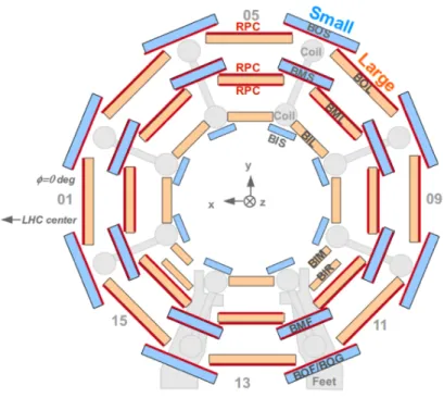
![Figure 1. Cross-sectional view of ATLAS in the r–z projection at φ = π/2, from ref. [ 1 ]](https://thumb-eu.123doks.com/thumbv2/9libnet/4077185.58243/4.892.189.694.147.451/figure-cross-sectional-view-atlas-projection-φ-ref.webp)


Benzer Belgeler
5) In the criticisms of Marx to a Russian sociologist M. In other words, Marx gave various kind of information about the political, economic, and social condition of the Asia,
Türk edebiyatında mekânı, özellikle çocukluğun yaşandığı evi, sanatçıyı besleyen bir unsur olarak ele alan ilk örnekler konusunda kesin bir görüşe sahip olmasak da
Bu çalışmada, daha çok sıçratmayı esas alan fiziksel buhar biriktirme yöntemleri üzerinde durulmuş ve manyetik alanda sıçratmanın temel bilgileri verilerek, bu
In the case of Israeli Palestinians conflict, the Lobby has to make sure that American power is used to support Israel and advance its interests in the Middle East region,
In government, secularism means a policy of avoiding entanglement between government and religion (ranging from reducing ties to a state religion to promoting secularism
Because of the filtration, some main solution holds on to the crystals, which remain on the filter paper, in this case it is removed by washing with a small amount of pure solvent.
Foreign language ictal speech automatism (FLISA) is a rare ictal sign in temporal lobe epilepsy arising from the non-dominant hemisphere.. While our literature review revealed no
The following were emphasized as requirements when teaching robotics to children: (1) it is possible to have children collaborate in the process of robotics design, (2) attention
