D O I: 1 0 .1 5 0 1 / C o m m u a 1 _ 0 0 0 0 0 0 0 7 9 1 IS S N 1 3 0 3 –5 9 9 1
RELIABILITY PROPERTIES OF THE SYSTEM CONSTRUCTED BY SWITCHING FROM ONE COMPONENT TO
TWO-DEPENDENT UNIT REDUNDANT STANDBY SYSTEM
MEHMET YILMAZ, MUHAMMET BEKÇI, AND BIROL TOPÇU
Abstract. In this work, we consider a system with switching towards to standby redundant system composed of two dependent components. Marginal distributions of component lifetimes are exponential and joint distribution be-longs to Farlie-Gumbel-Morgenstern family. We examine reliability properties of switching system such as shape of hazard rate function, mean residual life-time and some stochastic orders under determined circumstances on parameter spaces.
1. Introduction
Let T1 and T2be the component lifetimes whose joint distribution is the
bivari-ate Farlie-Gumbel-Morgenstern distribution with exponential marginals. The joint survival function of the components is given by
S (t1; t2) = S1(t1) S2(t2) [1 + F1(t1) F2(t2)]; ti> 0;
where 2 [ 1; 1] denotes association parameter, Si and Fi (i = 1; 2) are the
sur-vival and distribution functions of T1 and T2, respectively (Morgenstern 1956,[5]
Gumbel 1960, [3]). Throughout this study, it will be assumed that marginal distri-butions of the lifetimes are exponential with means i. Let D be a binary random
variable which determines the status of the switching device. Assume that D is a Bernoulli random variable with probability . Operation of this switching device is independent from the functioning of the components. While D = 1, unit1 conducts a task alone, and while D = 0, a parallel system, associatively composed of unit1 and unit2, carries out the task. So, changeover device switches from one component to two components in parallel. Let Tswdenote the lifetime of the system established
in this way, then it is clear that
Tsw= DT1+ (1 D) max fT1; T2g Received by the editors: May 15, 2016, Accepted: November 10, 2016.
2010 Mathematics Subject Classi…cation. Primary 60E15, 62H12; Secondary 60K10, 62N02. Key words and phrases. Switching system, Farlie-Gumbel-Morgenstern distribution, redun-dant system, hazard rate.
c 2 0 1 7 A n ka ra U n ive rsity C o m m u n ic a tio n s d e la Fa c u lté d e s S c ie n c e s d e l’U n ive rs ité d ’A n ka ra . S é rie s A 1 . M a th e m a t ic s a n d S t a tis tic s .
and hence the survival function of Tsw is found as
S (t) = P r (T1> t) P r (D = 1) + P r (max fT1; T2g > t) P r (D = 0) :
Based on the above de…nitions and assumptions, we clearly can rewrite S(t) as follows:
S (t) = S1(t) + (1 ) [1 F (t; t)]
The following examples can be given to illustrate the use of this system constructed in this manner in practice; waiting times of the customers serving in a multichannel queuing system with two associative servers ( secondary server is considered as a cold standby). The data of amount of water in the reservoir to be fed from at least one source. Supply-demand balance data in the production of a factory that has received a request from at least one customer. Lifetimes or recovery times data obtained from patients with two groups; such that, while the speci…c treatment is applied to …rst group, other appropriate treatment methods are also applied to second group in addition to the same treatment. Total duration data of movements in gold and dollar prices moving above a certain threshold level.
2. Distributional Properties
Let stand for the parameter vector ( 1; 2; ; ) then the distribution function
of the Tsw is given by
F (t; ) = F1(t; 1) + (1 ) fF1(t; 1) F2(t; 2) [1 + S1(t; 1) S2(t; 2)]g (2.1)
where Fi(t; i) = 1 e
t
i, (i = 1; 2) and Si = 1 Fi. Hence, by rewriting (2.1), we obtain F (t; ) = 1 e t1 + (1 ) n 1 e t1 1 e t 2 h 1 + e t1 e t 2 io = 1 e t1 + (1 ) e t 1 1+ 1 2 e t 2 + e t 11+ 1 2 e t 1 1+ 2 2 e t 2 1+ 1 2 + e 2t 1 1+ 1 2 (2.2) By di¤erentiating (2.2) and organizing obtained result, we have the probability density function as follows:
f (t; ) = 1 1 e t1 + (1 ) 1 2 e t2 1 1 + 1 2 e t 11+ 1 2 + (1 ) 1 1 + 2 2 e t 11+ 2 2 1 1 + 1 2 e t 11+ 1 2 + 2 1 + 1 2 e t 21+ 1 2 2 1 1 + 1 2 e 2t 11+ 1 2 (2.3)
We have the di¤erent shapes of the probability density function for various values of the switching probability and association parameter.
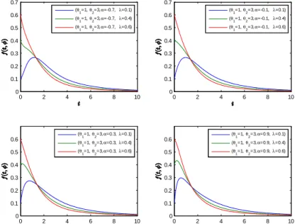
0 2 4 6 8 10 0 0.1 0.2 0.3 0.4 (θ 1=1,θ2=3,α=-0.7, λ=0.1) (θ 1=1,θ2=3,α=-0.1, λ=0.1) (θ 1=1,θ2=3,α=0.3,λ=0.1) (θ 1=1,θ2=3,α=0.9,λ=0.1) 0 2 4 6 8 10 0 0.1 0.2 0.3 0.4 0.5 (θ 1=1,θ2=3,α=-0.7, λ=0.4) (θ 1=1,θ2=3,α=-0.1, λ=0.4) (θ 1=1,θ2=3,α=0.3,λ=0.4) (θ 1=1,θ2=3,α=0.9,λ=0.4) 0 2 4 6 8 10 0 0.1 0.2 0.3 0.4 0.5 0.6 (θ 1=1,θ2=3,α=-0.7, λ=0.6) (θ 1=1,θ2=3,α=-0.1, λ=0.6) (θ 1=1,θ2=3,α=0.3,λ=0.6) (θ 1=1,θ2=3,α=0.9,λ=0.6) 0 2 4 6 8 10 0 0.2 0.4 0.6 0.8 1 (θ 1=1,θ2=0.3,α=-0.7, λ=0.1) (θ 1=1,θ2=0.3,α=-0.1, λ=0.1) (θ 1=1,θ2=0.3,α=0.3,λ=0.1) (θ 1=1,θ2=0.3,α=0.9,λ=0.1)
Figure 1. Shapes of the probability density function with respect to some values of association parameter.
0 2 4 6 8 10 0 0.1 0.2 0.3 0.4 0.5 0.6 0.7 (θ 1=1,θ2=3,α=-0.7, λ=0.1) (θ 1=1,θ2=3,α=-0.7, λ=0.4) (θ1=1,θ2=3,α=-0.7, λ=0.6) 0 2 4 6 8 10 0 0.1 0.2 0.3 0.4 0.5 0.6 0.7 (θ 1=1,θ2=3,α=-0.1, λ=0.1) (θ 1=1,θ2=3,α=-0.1, λ=0.4) (θ1=1,θ2=3,α=-0.1, λ=0.6) 0 2 4 6 8 10 0 0.1 0.2 0.3 0.4 0.5 0.6 (θ 1=1,θ2=3,α=0.3,λ=0.1) (θ1=1,θ2=3,α=0.3,λ=0.4) (θ 1=1,θ2=3,α=0.3,λ=0.6) 0 2 4 6 8 10 0 0.1 0.2 0.3 0.4 0.5 0.6 (θ 1=1,θ2=3,α=0.9,λ=0.1) (θ1=1,θ2=3,α=0.9,λ=0.4) (θ 1=1,θ2=3,α=0.9,λ=0.6)
Figure 2. Shapes of the probability density function with respect to some values of switching probabilities
The peaks of the probability density functions are ‡attened while probability of switching decreases (i.e. "). These begin to look like the exponential distribution. In addition, shape of the probability density function is quite di¤erent according to whether the mean life of a spare part is also be larger or smaller than the main part.
2.1. Moment generating function. The moment generating function of Tsw is
obtained as MTsw(v) = 1 1 1v + (1 ) (" 1 1 2v 1 1 1 2 1+ 2v # + " 1 1 1 2 1+2 2v 1 1 1 2 1+ 2v + 1 1 1 2 21+ 2v 1 1 1 2 2 1+2 2v #) ; where v < minn1 1; 1 2 o . Let k = E Tk
sw denote the kth raw moment then
k = k! 2 6 6 4 k1+ (1 ) 8 > > < > > : k 2 11 2+ 2 k + 1 2 1+2 2 k 1 + 1 2k 11 2+ 2 k + 1 2 2 1+ 2 k 9 > > = > > ; 3 7 7 5 :
2.2. Methods for random number generation. We will examine two cases according to the sign of the association parameter .
Case1. 1 0
Let’s rewrite the distribution function given with (2.1) in the following form; F (t) = F1(t) + (1 ) fF1(t)F2(t) [1 + + (1 F1(t)) (1 F2(t))]g
= F1(t) + (1 ) (1 + ) F1(t)F2(t)
+ (1 ) ( ) F1(t)F2(t) [1 (1 F1(t)) (1 F2(t))]
Then F (t) can be represented as a mixture of three distributions. Accordingly, com-ponent weights respectively are !1 = , !2 = (1 ) (1 + ), !3 = (1 ) ( )
with !1+ !2+ !3= 1 (!i 0). Consequently, the component distributions are;
G1(t) = F1(t) = Pr (T1 t) ;
G2(t) = F1(t)F2(t) = Pr =0(max fT1; T2g t) ;
G3(t) = F1(t)F2(t) [1 S1(t)S2(t)]
= Pr =0(max fT1; T2g t) Pr =0(min fT1; T2g t) ;
where the notation Pr =0( ) represents the case of independence of T1 and T2.
The distribution function given with (2.1), can be rewritten as
F (t) = F1(t) + (1 ) fF1(t)F2(t) [1 + + (1 F1(t)) (1 F2(t))]g
= F1(t) + (1 ) (1 ) F1(t)F2(t)
+ (1 ) F1(t)F2(t) [1 + (1 F1(t)) (1 F2(t))] :
Then we can see that F (t) can be represented by a mixture of three distributions such that the component weights are !1= , !2= (1 ) (1 ), !3= (1 )
with !1+ !2+ !3= 1 (!i 0). Accordingly, component distribution functions are
given by
G1(t) = F1(t) = Pr (T1 t) ;
G2(t) = F1(t)F2(t) = Pr =0(max fT1; T2g t) ;
G3(t) = F1(t)F2(t) [1 + S1(t)S2(t)] = Pr =1(max fT1; T2g t) :
Whereby, the following further steps to generate a random number from lifetime distribution of the system are given.
step1. Input parameter values 1; 2; ;
step2. Generate a random number u from uniform distribution on (0; 1) step3. If 0, then go to step4 otherwise go to step5;
step4.
If u , then F1(t) = u ) t = 1log (1 u),
else
If u + (1 ) (1 + ), then G2(t) = u ) t = G21(u). The following
calculations can be followed to the solution of the equation: Let = 1 e 1t then an appropriate solution for 2 [0; 1] can be obtained by the equation
1 (1 ) 12 = u. Hence t = 1log (1 ), else
Solve the equation G3(t) = u ) t = G31(u). This equation can be solved
with simple additional regulations such that by letting = 1 e 1t, then numerically solve the equation 1 (1 ) 12
h 1 (1 )(1 ) 12 i = u. Hence t = 1log (1 ). step5.
If u , then F1(t) = u ) t = 1log (1 u),
else
If u + (1 ) (1 ), then solve G2(t) = u ) t = G21(u)
i.e. solve 1 (1 ) 12 = u then t = 1log (1 ), else
Solve the equation G3(t) = u ) t = G31(u),
i.e. solve 1 (1 ) 12 h 1 + (1 )(1 ) 12 i = u then t = 1log (1 ).
Detailed information about a number generation by inverse method, and a number generation from mixed distribution, can be found in Gentle (2004), [2]
2.3. Parameter estimations by maximum likelihood. Let t1; t2; :::; tn be the
observed lifetimes of size n from the system. Then the log-likelihood function is given by log L ( 1; 2; ; ;t) = n P i=1 log f1(ti; 1) + (1 ) f1(ti; 1) f2(ti; 2) [1 + (2F1(ti; 1) 1) (2F2(ti; 2) 1)] = n P i=1 log (f1(ti; 1)) + n P i=1 log + (1 ) f2(ti; 2) [1 + (2F1(ti; 1) 1) (2F2(ti; 2) 1)] (2.4) By di¤erentiating (2.4) with respect to ( 1; 2; ; ) then we have
@ log L @ 1 = n X i=1 @ @ 1 log (f1(ti; 1)) +2 (1 ) n X i=1 @F1(ti; 1) @ 1 f2(ti; 2) (2F2(ti; 2) 1) ( + (1 ) f2(ti; 2) [1 + (2F1(ti; 1) 1) (2F2(ti; 2) 1)]) @ log L @ 2 = (1 ) n X i=1 @f2(ti; 2) @ 2 [1 + (2F1(ti; 1) 1) (2F2(ti; 2) 1)] ( + (1 ) f2(ti; 2) [1 + (2F1(ti; 1) 1) (2F2(ti; 2) 1)]) + (1 ) n X i=1 2 f2(ti; 2)@F2@(ti2; 2)(2F1(ti; 1) 1) ( + (1 ) f2(ti; 2) [1 + (2F1(ti; 1) 1) (2F2(ti; 2) 1)]) @ log L @ = (1 ) n X i=1 f2(ti; 2) [(2F1(ti; 1) 1) (2F2(ti; 2) 1)] ( + (1 ) f2(ti; 2) [1 + (2F1(ti; 1) 1) (2F2(ti; 2) 1)]) @ log L @ = n X i=1 1 f2(ti; 2) [1 + (2F1(ti; 1) 1) (2F2(ti; 2) 1)] ( + (1 ) f2(ti; 2) [1 + (2F1(ti; 1) 1) (2F2(ti; 2) 1)])
By equating above system of equations to zero, then we obtain the maximum like-lihood estimates b = b1; b2; ^; ^ by solving numerically this nonlinear system of
2.4. Estimating by EM algorithm. The p.d.f of Tsw can be represented by a
mixture of two p.d.fs as the following form:
fTsw(t; 1; 2; ; w1; w2) = w1f1(t; 1) + w2f12(t; 1; 2; ); w1+ w2= 1 where f1 stands for p.d.f of Exp( 1)and f12 stands for p.d.f of (T1; T2). We use
Lagrange multipliers to solve a constrained maximization problem. log L ( 1; 2; ; w1; w2;t) = n X i=1 log (w1f1(ti; 1) + w2f12(ti; 1; 2; )) " (w1+ w2 1) (2.5)
Straightforwardly, we get the system of equations, by di¤erentiating (2.5) with respect to ( ; w1; w2) and equating it to zero, as follows:
@ log L @ 1 = n P i=1 w1@ 1@ f1(ti; 1)+w2@ 1@ f12(ti; 1;2; ) (w1f1(ti; 1)+w2f12(ti; 1;2; )) = n P i=1 w1f1(ti; 1)@ 1@ log(f1(ti; 1))+w2f12(ti; 1;2; )@ 1@ log(f12(ti; 1; 2; )) (w1f1(ti; 1)+w2f12(ti; 1;2; )) = n P i=1Pr ( 1j t i)@@1log (f1(ti; 1)) + n P i=1Pr ( 2j t i)@@1log (f12(ti; 1; 2; )) = 0 (2.6) @ log L @ 2 = n P i=1 w2@ 2@ f12(ti; 1; 2; ) (w1f1(ti; 1)+w2f12(ti; 1; 2; )) = n P i=1 w2f12(ti; 1;2; )@ 2@ (log f12(ti; 1; 2; )) (w1f1(ti; 1)+w2f12(ti; 1;2; )) = n P i=1Pr ( 2j t i)@@2(log f12(ti; 1; 2; )) = 0 (2.7) @ log L @ = n P i=1 (w2@@f12(ti; 1; 2; )) (w1f1(ti; 1)+w2f12(ti; 1; 2; )) = n P i=1 w2f12(ti; 1; 2; )@@ log(f12(ti; 1; 2; )) (w1f1(ti; 1)+w2f12(ti; 1; 2; )) = n P i=1Pr ( 2j t i)@@ log (f12(ti; 1; 2; )) = 0 (2.8) @ log L @w1 = n X i=1 f1(ti; 1) (w1f1(ti; 1) + w2f12(ti; 1; 2; )) " = 0 (2.9) @ log L @w2 = n X i=1 f12(ti; 1; 2; ) (w1f1(ti; 1) + w2f12(ti; 1; 2; )) " = 0 (2.10)
If both sides of the last two equations are multiplied by w1 and w2, respectively
and by taking summation of both terms, then we have
n P i=1 w1f1(ti; 1) (w1f1(ti; 1)+w2f12(ti; 1; 2; ))+ n P i=1 w2f12(ti; 1;2; ) (w1f1(ti; 1)+w2f12(ti; 1; 2; )) " (w1+ w2) = 0 = n P i=1 w1f1(ti; 1)+w2f12(ti; 1; 2; ) (w1f1(ti; 1)+w2f12(ti; 1; 2; )) " = 0
This implies " = n. Hereby, equation (2.9) or (2.10) yields EM estimates of as ^ =
1 n n P i=1Pr ( 1j t i). If initial values 01; 0 2; 0; 0
are given, then Pr ( 1j xi) and Pr ( 2j xi)
are calculated. Consequently, solving the equations (2.6)-(2.8) numerically gives updated values of parameters. This step is repeated iteratively until convergence is detected.
Everitt and Hand (1981), [1] may be seen as a source for further reading about using EM algorithm for mixed distributions.
3. Reliability Properties
In this subsection we introduce the reliability function, the hazard rate function and the mean residual life function for this switching system.
3.1. Reliability function. Let Si(t) = 1 Fi(t) stand for the survival function of
i:th component lifetime then the survival function of Tsw is given by
S(t) = S1(t) + (1 ) f1 F1(t)F2(t) [1 + S1(t)S2(t)]g
Since the marginal survival functions are e t1 and e t 2 we have S(t) = e t1 + (1 ) n 1 1 e t1 1 e t 2 h 1 + e t1 e t 2 io = e t1 + (1 ) e t 2 1 e t 1 (1 ) e t 1 1+ 1 2 n 1 e t1 1 e t 2 o (3.1) It can be concluded that when two components are negatively associated, high switching probability can raise the survival probability of the system.
Even if mean lifetime of the spare part is short, these still work with higher proba-bility when they are connected together in parallel. According to these conditions, it will also be attractive for us to examine the behavior of the system’s failure rate function.
3.2. Hazard rate function. The failure or hazard rate function is de…ned by r(t) = dtd log (S(t)) = f (t)S(t). Accordingly, from the expressions (2.3) and (3.1), hazard rate function of Tsw is given by
r(t) = 1 1 1 + (1 ) 1 2 ( (1 2)e t(1 1) 1 ) + ( 2 1e t(1 2) 1+( 1+ 2)e t(1 1) (21+ 2)e t(1 1+ 12) ) et( 1 2)+(1 ) " e t 1 1 + e t( 1 2) 1+e t( 1 1) e t( 1 1+ 12) !# i (3.2)
The hazard rate of the system exhibits ‡exibility according to the switch transition probability and association parameter . In this context, our intent to examine the reliability properties such as failure rate and mean residual life of the system, and obtain some orderings.
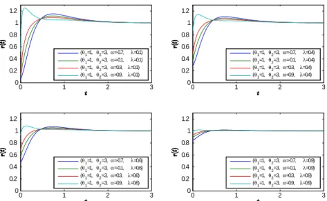
0 2 4 6 8 0 0.1 0.2 0.3 0.4 0.5 0.6 0.7 (θ 1=1,θ2=3,α=-0.7, λ=0.1) (θ 1=1,θ2=3,α=-0.1, λ=0.1) (θ 1=1,θ2=3,α=0.3,λ=0.1) (θ 1=1,θ2=3,α=0.9,λ=0.1) 0 2 4 6 8 0 0.2 0.4 0.6 0.8 1 (θ 1=1,θ2=3,α=-0.7, λ=0.4) (θ 1=1,θ2=3,α=-0.1, λ=0.4) (θ 1=1,θ2=3,α=0.3,λ=0.4) (θ 1=1,θ2=3,α=0.9,λ=0.4) 0 2 4 6 8 0 0.2 0.4 0.6 0.8 1 (θ 1=1,θ2=3,α=-0.7, λ=0.6) (θ 1=1,θ2=3,α=-0.1, λ=0.6) (θ 1=1,θ2=3,α=0.3,λ=0.6) (θ 1=1,θ2=3,α=0.9,λ=0.6) 0 2 4 6 8 0 0.2 0.4 0.6 0.8 1 (θ 1=1,θ2=3,α=-0.7, λ=0.9) (θ 1=1,θ2=3,α=-0.1, λ=0.9) (θ 1=1,θ2=3,α=0.3,λ=0.9) (θ 1=1,θ2=3,α=0.9,λ=0.9)
Figure 3. Shapes of the hazard rate function with respect to some values of association parameter.
0 2 4 6 8 0 0.2 0.4 0.6 0.8 1 (θ1=1,θ2=3,α=-0.9, λ=0.1) (θ1=1,θ2=3,α=-0.9, λ=0.3) (θ1=1,θ2=3,α=-0.9, λ=0.5) (θ1=1,θ2=3,α=-0.9, λ=0.8) 0 2 4 6 8 0 0.2 0.4 0.6 0.8 1 (θ1=1,θ2=3,α=-0.6, λ=0.1) (θ1=1,θ2=3,α=-0.6, λ=0.3) (θ1=1,θ2=3,α=-0.6, λ=0.5) (θ1=1,θ2=3,α=-0.6, λ=0.8) 0 2 4 6 8 0 0.2 0.4 0.6 0.8 1 (θ1=1,θ2=3,α=.6,λ=0.1) (θ1=1,θ2=3,α=.6,λ=0.3) (θ1=1,θ2=3,α=.6,λ=0.5) (θ1=1,θ2=3,α=.6,λ=0.8) 0 2 4 6 8 0 0.2 0.4 0.6 0.8 1 (θ1=1,θ2=3,α=0.9,λ=0.1) (θ1=1,θ2=3,α=0.9,λ=0.3) (θ1=1,θ2=3,α=0.9,λ=0.5) (θ1=1,θ2=3,α=0.9,λ=0.8)
Figure 4. Shapes of the hazard rate function with respect to some values of switching probability.
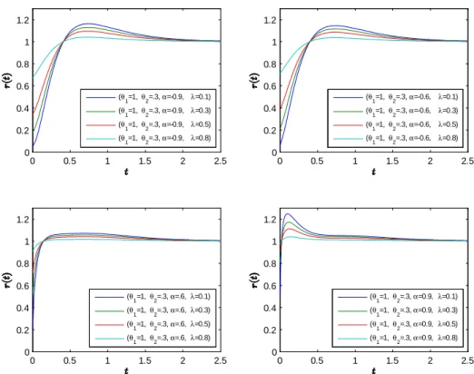
0 1 2 3 0 0.2 0.4 0.6 0.8 1 1.2 (θ1=1,θ2=.3,α=-0.7, λ=0.1) (θ1=1,θ2=.3,α=-0.1, λ=0.1) (θ1=1,θ2=.3,α=0.3, λ=0.1) (θ1=1,θ2=.3,α=0.9, λ=0.1) 0 1 2 3 0 0.2 0.4 0.6 0.8 1 1.2 (θ1=1,θ2=.3,α=-0.7, λ=0.4) (θ1=1,θ2=.3,α=-0.1, λ=0.4) (θ1=1,θ2=.3,α=0.3, λ=0.4) (θ1=1,θ2=.3,α=0.9, λ=0.4) 0 1 2 3 0 0.2 0.4 0.6 0.8 1 1.2 (θ1=1,θ2=.3,α=-0.7, λ=0.6) (θ1=1,θ2=.3,α=-0.1, λ=0.6) (θ1=1,θ2=.3,α=0.3, λ=0.6) (θ1=1,θ2=.3,α=0.9, λ=0.6) 0 1 2 3 0 0.2 0.4 0.6 0.8 1 1.2 (θ1=1,θ2=.3,α=-0.7, λ=0.9) (θ1=1,θ2=.3,α=-0.1, λ=0.9) (θ1=1,θ2=.3,α=0.3, λ=0.9) (θ1=1,θ2=.3,α=0.9, λ=0.9)
Figure 5. Shapes of the hazard rate function with respect to some values of association parameter (mean lifetime of second component is less than main component).
0 0.5 1 1.5 2 2.5 0 0.2 0.4 0.6 0.8 1 1.2 (θ1=1,θ2=.3,α=-0.9, λ=0.1) (θ1=1,θ2=.3,α=-0.9, λ=0.3) (θ1=1,θ2=.3,α=-0.9, λ=0.5) (θ1=1,θ2=.3,α=-0.9, λ=0.8) 0 0.5 1 1.5 2 2.5 0 0.2 0.4 0.6 0.8 1 1.2 (θ1=1,θ2=.3,α=-0.6, λ=0.1) (θ1=1,θ2=.3,α=-0.6, λ=0.3) (θ1=1,θ2=.3,α=-0.6, λ=0.5) (θ1=1,θ2=.3,α=-0.6, λ=0.8) 0 0.5 1 1.5 2 2.5 0 0.2 0.4 0.6 0.8 1 1.2 (θ1=1,θ2=.3,α=.6,λ=0.1) (θ1=1,θ2=.3,α=.6,λ=0.3) (θ1=1,θ2=.3,α=.6,λ=0.5) (θ1=1,θ2=.3,α=.6,λ=0.8) 0 0.5 1 1.5 2 2.5 0 0.2 0.4 0.6 0.8 1 1.2 (θ1=1,θ2=.3,α=0.9,λ=0.1) (θ1=1,θ2=.3,α=0.9,λ=0.3) (θ1=1,θ2=.3,α=0.9,λ=0.5) (θ1=1,θ2=.3,α=0.9,λ=0.8)
Figure 6. Shapes of the hazard rate function with respect to some values of switching probability (mean lifetime of second component is less than main component).
3.3. Mean residual life function. The mean residual life of the certain part of age x is de…ned as the expected value of remaining life of the part (Lai and Xie 2006, [4]). Hence, (x) = E(Tsw xjTsw> x) = R1 x STsw(t)dt STsw(x) = 1+(1 ) 1 2 1 + 2e x 2 2 4 1 + 2 1 e x 1 1 8 < :1 2 1+ 21 + 2e x 2 1 + 2 1 +2 2e x 1+e x( 1 1+ 12) 2 9 = ; 3 5 1+(1 )e x 2 " e x 1 1 ( 1 e x 2 e x 1+e x( 1 1+ 12) )# : (3.3)
4. Some Orderings
Throughout this section, we will assume that component lifetimes are identical i.e.
1= 2. Stochastic and hazard rate orderings are investigated based on association
parameter and switching probability .
4.1. Stochastic ordering. Stochastic relationship will be investigated according to the monotonicity of or . First, let’s look at the de…nition of stochastic ordering;
De…nition 1: Let X and Y be two random variables de…ned on the same sup-port, then X is said to be stochastically smaller than Y , denoted by X stY ) if
Pr (X > x) Pr (Y > x) holds 8x 2 ( 1; 1) (Shaked and Shanthikumar 2007, [6]).
According to this de…nition, survival function of Tsw is rewritten below by taking
e t = u for the simplicity;
S(u; ; ) = u [1 + (1 ) (1 u) f1 u (1 u)g] (4.1)
Firstly, we consider the case of < 0. It can be easily seen that, regardless of
the sign of , S 0(u) S (u) holds for all u. Hence a stochastic relationship T(
0; )
sw stTsw( ; ) exists for < 0. According to existing relationship, we can say
that the lifetime of the system composed of two identical but negatively associated components regardless of the switching probability is longer.
Secondly, we consider the case of < 0. If someone thinks about visual representa-tion of the system, then it will be seen immediately that an increment in switching probability gets a longer lifetime of the system. It is obvious from the statement (4.1) that S 0(u) S (u) holds. Hence T(
; 0)
sw stTsw( ; )holds. If the components
are connected to parallel with regardless of the association parameter, then they extend the lifetime of the system.
Now, we will investigate a relationship when both the association parameter and the switching probability have a simultaneous increment. Namely, we consider the case of < 0 and < 0. Let’s consider the ratio S 0; 0(u) S ; (u)
u(1 u) . Then
S 0; 0(u) S ; (u)
u (1 u) =
0 + u (1 u) (1 ) 0 1 0 :
By noting that u (1 u) 1 holds, then we conclude that
0 + (1 ) 0 1 0 = (1 0) 1 0 (1 ) (1 )
(1 0) (1 ) (1 ) (1 )
= (1 ) [ 0 ] 0
namely, the sign of this ratio is negative. Hence S 0; 0(u) S ; (u) i.e. T( 0; 0)
sw
4.2. Hazard rate orderings.
:
De…nition 2: Let X and Y be two random variables de…ned on the same support of x, respectively rX and rY denote the hazard rates. If rY (x) rX(x) holds for
all x 2 ( 1; 1), then X is said to be smaller than Y in the hazard rate order, and this relationship is denoted by X hrY . (Shaked and Shanthikumar 2007, [6]).
As seen from these …gures (3-6), ordering may exist only for switching probability. However, in terms of being misleading we will …rst be investigated a relationship for < 0. By letting e t = u in statement (3.2), then we have
r (u) =1 1(1 ) u 2 4 1 + (1 u) (1 3u) (2 ) (1 ) uh1 + (1 u)2i 3 5 : (4.2)
We decide the monotonicity of (4.2) by taking …rst derivative of r(u) with respect to . Hence d d r(u) = 1 (1 ) u (1 u) h (2 ) (1 ) u h 1 + (1 u)2 ii2 2 (1 ) u2 3 (2 ) u + (2 ) :
The last multiplier in the statement above is a convex function of u. Furthermore, its value is 2 > 0 for u = 0 and 2 for u = 1. Thus, one of the roots of a quadratic polynomial should be in the range (0; 1). The roots of this polynomial respectively are
u1;2=
3 (2 ) p(2 ) (10 )
4 (1 ) :
Now, u1will be checked whether it is in [0; 1]. Positivity of u1 is obvious from the
statement below
9(2 )2 (2 ) (10 ) = (2 ) [9 (2 ) (10 )] = 8 (2 ) (1 ) 0:
It will be checked whether it is less than 1. For this, positivity of the following statement is
3 (2 ) 4 (1 ) p(2 ) (10 )
which implies
(2 + )2 (2 ) (10 ) = 16 (1 ) 0:
In this case, the sign of derivative changes its direction at least once. Therefore, the hazard rate ordering is not valid according to association parameter. Now, we will investigate the existence of the relationship for < 0. By rearranging r (u) as below: r (u) = 1 1u 2 4 1 + (1 u) (1 3u) (2 ) (1 ) u h 1 + (1 u)2i 3 5 ;
then statement (2 ) = (1 ) = 1 + 1= (1 ) in brackets increases in . r (u) also increases in as long as nominator in brackets is positive. (1 u) (1 3u) is a convex function and it equals 1 when u = 0, it is equals 0 when u = 1. The minimum value of this convex function is 1
3 which is attained at 2
3. According to
this, since (1 u) (1 3u) 3 holds for 0, 1 3 0 is valid. On the
other hand, (1 u) (1 3u) 1 implies 1 + (1 u) (1 3u) 1 + 0 holds for < 0. In this case, we obtain r (u) r 0(u) for < 0 which implies that T( ;
0)
sw hrTsw( ; )is valid.
Whatever the association parameter is higher switching probability makes the sys-tem more preferable in terms of the hazard rate.
5. Applications
In this section, we want to illustrate the usefulness of the model by using two real data sets.
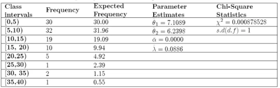
Data Set 1. This data set includes customer waiting times and considered as grouped data by Shanker et.al (2013) [7]. They have proposed two-parameter Lind-ley distribution to …t waiting times (in minutes) of 100 bank customers in the queue. They have calculated Chi-Square Statistics for both Lindley and two-parameter Lindley distributions, which respectively are 0:09402 and 0:07482. Similarly, we apply goodness-of-…t to this grouped data by considering our model.
As it is thought to be …ction; the system is running with one booth attendant, but occasionally, another one also serves the customer to help.
Chi-Square goodness of …t test results and the expected frequencies can be obtained as follows:
TABLE 1. Frequency table of waiting times of 100 bank customers.
The main booth attendant serves the customers with an average of 7 minutes, and the other one serves with an-average of 6 minutes. Also, it said that, they were working together in general along the days but independently. According to Lindley types, quite small chi-square statistics were obtained with this model.
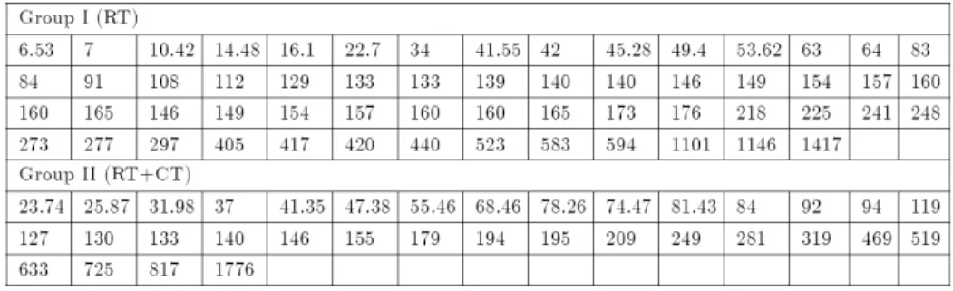
Data Set 2. The two data sets in Table 2 represent the survival times (in days) of two groups of patients su¤ering from head and neck cancer disease. Group 1 was treated using radiotherapy (RT), whereas the patients belonging to Group 2 were
treated using a combined radiotherapy and chemotherapy (CT). These data set are taken from Sharma et. al (2015), [8].
TABLE 2.Survival times of patients (RT,RT+CT)
We merge the survival times of the patients belonging to Group 1 and 2. We apply the model to …t single data set. Maximum Likelihood Estimates and Kolmogorov-Smirnov statistic for the suggested model parameters are tabulated as follows:
TABLE 3. Estimates of the parameters and Kolmogorov-Smirnov Statistic (K-S)
Most of patients had only been applied only treatment, the e¤ect of the combined treatment is particularly e¤ective in the positive direction.
References
[1] Everitt, B.S., and Hand, D.J. (1981). Finite Mixture Distributions, Chapman and Hall, Lon-don.
[2] Gentle, J.E. (2004). Random Number Generation and Monte Carlo Methods (Statistics and Computing) 2nd Edition, Springer.
[3] Gumbel, E. J. (1960). Bivariate exponential distributions, Journal of American Statistical Association, 55, pp. 698-707.
[4] Lai, C. D., and Xie, M. (2006). Stochastic ageing and dependence for reliability. Springer Science & Business Media.
[5] Morgenstern, D. (1956). Einfache Beispiele zweidimensionaler Verteilungen, Mitteilungsblatt fuÈr Mathematische Statistik, 8, pp. 234-235.
[6] Shaked, M., and Shanthikumar, J. G. (2007). Stochastic orders. Springer Science & Business Media.
[7] Shanker, R., Sharma, S., Shanker, R. (2013). A Two-Parameter Lindley Distribution for Mod-eling Waiting and Survival Times Data, Applied Mathematics, 4, 363-368.
[8] Sharma, V.K., Singh, S.K., Singh, U., Agiwal, V. (2015). The inverse Lindley distribution: a stress-strength reliability model with application to head and neck cancer data, Journal of Industrial and Production Engineering, 32:3, 162-173, DOI: 10.1080/21681015.2015.1025901
Current address : Ankara University, Faculty of Sciences, Department of Statistics , Ankara, Turkey.
E-mail address, Mehmet Y¬lmaz: [email protected] E-mail address, Muhammet Bekçi: [email protected] E-mail address, Birol Topçu: [email protected]