Kahramanmaras Sutcu Imam University
Journal of Engineering Sciences
Geliş Tarihi :25.06.2020 Received Date : 25.06.2020
Kabul Tarihi :25.09.2020 Accepted Date : 25.09.2020
BİTKİLERDE DURAYLI CİVA İZOTOPLARININ AYRIMLILAŞMASI
STABLE MERCURY ISOTOPE FRACTIONATION BEHAVIOURS OF PLANTS
Ayça DOĞRUL SELVER 1 (ORCID: 0000-0002-9003-5439
)
1 Kahramanmaraş Sütçü İmam Üniversitesi, Jeoloji Mühendisliği Bölümü, Kahramanmaraş, Türkiye
*Sorumlu Yazar / Corresponding Author: Ayça DOĞRUL SELVER, [email protected]
ÖZET
Bu çalışmanın ana amacı farklı fotosentez tiplerine sahip bitkilerde (C3, C4 ve CAM) civa (Hg) izotop davranışlarının belirlenmesi ve bitkilerin farklı kısımlarının Hg izotopları açısından farklılık gösterip göstermediğinin incelenmesidir. Bu amaçla, bitkilerin karbon izotopları analiz edilmiş ve böylece fotosentetik tipleri belirlenmiştir. Daha sonra bitkiler yaprak, sap ve kök olarak faklı kısımlara ayrılmış ve bu kısımların Hg izotopları analiz edilmiştir. C3 ve C4 bitkilerinde çift kütle numaralı civa izotopları kütleye bağımlı (MDF), tek kütle numaralı izotoplar ise kütleden bağımsız ayrımlılaşma (MIF) göstermiştir. Hem C3 hem de C4 bitkilerinin hafif Hg izotoplarınca zenginleştiği fakat kütleye bağlı ayrımlılaşmanın C3 bitkilerinde C4 bitkilerinden yaklaşık 3 kat fazla olduğu belirlenmiştir. Hem C3 hem C4 bitkileri negative MIF göstermiştir. Çalışmada sadece 1 adet CAM bitkisi analiz edilmiş ve bu CAM bitkisinin ağır Hg izotoplarınca az miktarda zenginleşme gösterdiği ve belirgin bir negative MIF göstermediği belirlenmiştir. Bu bulgular, Hg izotop bileşimi ve bitkilerin fotosentez tipi arasında bir ilişki olduğuna işaret etmektedir.
Ek olarak, bitkilerin yapraklarının köklerine kıyasla biraz daha fazla ayrımlılaştığı bulunmuş ve bu farkın yaprak ve köklerin Hg kaynaklarının farklı olmasından kaynaklandığı öne sürülmüştür.
Anahtar Kelimeler: Civa izotopları, kütleden bağımsız ayrımlılaşma, fotosentez tipleri, izotop ayrımlılaşması ABSTRACT
The overarching aim of this study is to define mercury (Hg) isotopic features of plants which have different photosynthetic pathways (C3, C4 and CAM) and to understand if different parts of the plants have different Hg isotopic fractionation behavior. For this, carbon isotopic values of terrestrial plants were analyzed which were used to determine the photosynthetic pathways of plants. Plants were sub-sampled into leaves, stems and roots and their Hg isotopic values were analyzed.
Results showed that C3 and C4 plants exhibit mass dependent (even Hg isotopes) and mass independent Hg isotope fractionation (odd Hg isotopes). Both C3 and C4 plants are enriched in light isotopes, but the degree of mass fractionation is approximately three times greater in C3 plants, than in C4 plants. Hg in both C3 and C4 plants exhibit negative MIF isotope effect which reported as depletion “and no clear MIF effect. These findings suggest a connection between the Hg isotopic composition and the photosynthetic pathway.
In addition, the leaves are slightly more fractionated than the roots. Differences in the degree of MIF between roots and leaves suggest that they obtain Hg from different sources.
Keywords: Mercury isotopes, mass independent fractionation, photosynthetic pathways, isotope fractionation
ToCite: DOĞRUL SELVER, A., (2020).
STABLE MERCURY ISOTOPE FRACTIONATION BEHAVIOURS OF PLANTS. Kahramanmaraş Sütçü İmam Üniversitesi Mühendislik Bilimleri Dergisi, 23(4), 197-209.INTRODUCTION
Mercury (Hg) is a toxic global pollutant and it can be emitted to the atmosphere by natural and anthropogenic processes (Driscoll, Mason, Chan, Jacob, & Pirrone, 2013; Lamborg et al., 2002; Pirrone, Keeler, & Nriagu, 1996; Schroeder, 1998). The elemental gaseous form of Hg has long residence time (~1yr) in the atmosphere (Schroeder, 1998) therefore it can be transported long distances before being oxidized or deposited (Durnford, Dastoor, Figueras-Nieto, & Ryjkov, 2010; Lindberg et al., 2007). In addition when Hg is methylated, it becomes bioaccumulative which then poses a serious health problems. Therefore, to gain understanding of the source, fate and transformation of Hg in the environment is important. Studies to date showed that different natural samples vary in their Hg isotope compositions which suggest the use of Hg isotopes for source fingerprinting and for understanding transformation reactions.
Hg has seven stable isotopes whose relative abundances are 196 Hg (0.15%), 198Hg (9.97 %), 199Hg (16.87 %), 200Hg
(23.1 %), 201Hg (13.18%), 202Hg (29.86%), and 204Hg (6.86%) (Zadnik, Specht, & Begemann, 1989). Hg isotopes
have been extensively used to understand fractionation behavior of different Hg isotopes in various natural samples (Biswas, Blum, Bergquist, Keeler, & Xie, 2008; Cai & Chen, 2016; Das, Salters, & Odom, 2009; S Ghosh, Xu, Humayun, & Odom, 2008; Zheng, Obrist, Weis, & Bergquist, 2016) and to trace Hg contaminant sources (Hintelmann & Zheng, 2011; Yin, Feng, Li, Yu, & Du, 2014). On the other hand, studies on Hg isotopes in terrestrial and aquatic vegetation is limited (Carignan, Estrade, Sonke, & Donard, 2009; S Ghosh et al., 2008; Sulata Ghosh, 2010; Yin, Feng, & Meng, 2013).
Mercury isotopes show both mass dependent (MDF) and mass independent isotope fractionation (MIF). Among seven Hg isotopes, even numbered Hg isotopes (especially 202Hg) show MDF .On the other hand, odd isotopes of
Hg (199Hg and 201Hg) usually undergo MIF and produce negative isotopic anomalies (expressed as Δ199Hg and
Δ201Hg). Δ199Hg and Δ201Hg are a measure of the deviation from predicted MDF line. In 2007, Bergquist and Blum
reported MIF of Hg isotopes in fish samples and reported up to 2.5‰ fractionation in odd Hg isotopes. Following to this study, MIF of odd Hg isotopes has been found in many natural samples such as sediments (Donovan, Blum, Yee, Gehrke, & Singer, 2013; Foucher, Hintelmann, Al, & MacQuarrie, 2013; Gehrke, Blum, & Marvin-DiPasquale, 2011), atmospheric samples (Sulata Ghosh, 2010; Yin et al., 2013; Yuan et al., 2015), lichens and mosses (Blum et al., 2012; S Ghosh et al., 2008; Sulata Ghosh, 2010). Photodegradation, photochemical reduction, abiotic reduction and evaporation are the mechanisms which are suggested to cause MIF (Bergquist & Blum, 2007; Sanghamitra Ghosh, Schauble, Lacrampe Couloume, Blum, & Bergquist, 2013; Zheng & Hintelmann, 2010).
The magnetic isotope effect (MIE) and the nuclear volume effect (NVE) are the most probable mechanisms causing MIF of odd isotope.
NVE is related with the nuclear volume and radius which is not proportional to the mass number. Isotopes have same charge but different neutron numbers and therefore a change in the neutron number result in the change in nuclear charge distribution which ultimately result in NVE. For heavier isotopes (lower nuclear charge density), the nuclear charge is distributed over a bigger volume while for smaller isotopes it is distributed over a small volume (higher nuclear charge density). On the other hand, odd isotopes have different behaviors, because of the nuclear energy splitting in the spectral lines. The MIE occurs when there is a spin-selective chemical reaction and it sorts nuclei according to their spins and magnetic moments (Buchachenko et al, 1976, Buchachenko, 2000). Among seven isotopes, even isotopes are spinless and non-magnetic but odd isotopes (199Hg and 201Hg) have non zero nuclear spins
and magnetic moments therefore MIE only affects the odd isotopes. The result of magnetic isotope effect is fractionation of magnetic and non-magnetic isotopes in a chemical reaction (Buchachenko, 2000) and this depends on nuclear spin quantum number.
In this study, carbon and Hg isotope ratios of terrestrial plants were analyzed and interpreted together to understand (a) if there is any difference in Hg isotope signatures of plant samples which have different photosynthetic pathways (b) if there is a difference in the Hg isotopic fractionation in different parts of plants (mainly roots and leaves) (c) if
MDF and MIF occurs in terrestrial plants. METHOD
Sampling and Sample Preparation
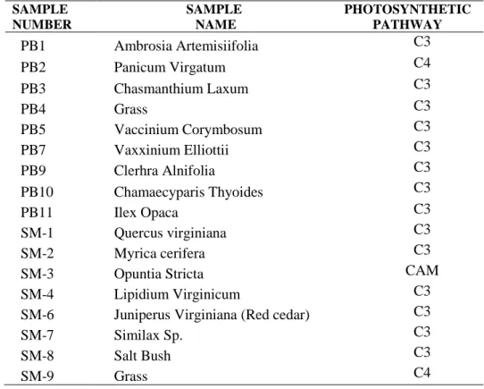
Plant samples were collected in St. Marks Wildlife Refuge, Florida and in Black Water River State Park, Pensacola, Florida. İdentification of plant samples were done by Dr. Loren Anderson in the Department of Biology at FSU and by experts in Tallahassee Nurseries (Table 1).
Plants were divided into three sub-samples: leaves, stems and roots if available. Some of the plants were trees, and tree roots could not be collected in St. Marks Wildlife Refuge. Upon arrival to laboratory, each part was cleaned with Kimwipes to get rid of dust, soil and other particles. After being freeze dried, plant samples were ground into powder for further sample preparation.
For the carbon isotopic measurements, approximately 100 micrograms of ground plant samples were put in tin capsules.
For the mercury isotopic measurement, 2-3 grams of ground freeze dried sample was dissolved in aqua regia (3:1 14 N HNO3 to 12 N HCl) and left on the hot plate (~50C) for 8 hours and at room temperature for 7 days. At the
end of 7 days, this solution was filtered through 100 micron filter paper. After filtering the samples, concentrated NaOH is added to solutions to reduce the acidity.
Table 1. Numbers, Names and Photosynthetic Pathways of Samples (PB: Pensacola Blackwater River Park Samples, SM: St. Mark’s Samples)
SAMPLE NUMBER SAMPLE NAME PHOTOSYNTHETIC PATHWAY PB1 Ambrosia Artemisiifolia C3 PB2 Panicum Virgatum C4 PB3 Chasmanthium Laxum C3 PB4 Grass C3 PB5 Vaccinium Corymbosum C3 PB7 Vaxxinium Elliottii C3 PB9 Clerhra Alnifolia C3 PB10 Chamaecyparis Thyoides C3 PB11 Ilex Opaca C3 SM-1 Quercus virginiana C3 SM-2 Myrica cerifera C3
SM-3 Opuntia Stricta CAM
SM-4 Lipidium Virginicum C3
SM-6 Juniperus Virginiana (Red cedar) C3
SM-7 Similax Sp. C3
SM-8 Salt Bush C3
SM-9 Grass C4
Instrumental Analyses Mercury Isotopic Analyses
Mercury isotopic analysis methodology is developed by Ghosh, 2008. The sample solution was introduced to Thermo Finnigan Neptune multi collector inductively coupled plasma by a CETAC HGX-200 cold vapor hydride generator (in NHMFL, Florida State University). Sample solution is introduced into the hydride generator along with
1-2 % SnCl2 in a 1N HCl matrix to reduce the divalent mercury (Hg+2) in the solution and releases elemental mercury
into gaseous phase. This cold vapor is introduced into the MC-ICP-MS to measure mercury isotopic ratios.
The 1 ppb mercury standard which was diluted from the 10 ppm standard reference material of National Institute of Standards and Technology (NIST SRM 3133) was used during analysis.
Seven adjustable Faraday cups were used for mercury isotope ratio measurements for mass numbers of 198, 199, 200, 201, 202, and 204 and also 204Pb interference on 204 Hg was monitored at 206. Raw isotope ratios of 198Hg/200Hg, 199Hg/200Hg, 201Hg/200Hg, 202Hg/200Hg and 204Hg/200Hg were calculated from the respective ion currents. For
minimizing effects of instrumental fractionation, isotope ratios were determined by sample standard bracketing technique. Hg isotope ratios are reported relative to NIST-3133 Hg standard in δ (‰) notation (Eq.1);
1000
1
3133 200 200
NIST A SAMPLE A NHg
Hg
Hg
Hg
Hg
(1)where A is the mass of each Hg isotope between 199 and 204 amu. Carbon Isotopic Analyses
For the carbon isotopic measurements, ground plant samples are put in tin capsules and loaded in the auto-sampler of a Carlo Erba Elemental Analyzer (EA) that is interfaced to a Finnigan MAT delta Plus XP stable isotope ratio mass spectrometer (IRMS). The sample is first introduced into the combustion column of the EA to produce a gas mixture of CO2, N2, SO3, SO2, NxOx and etc. The gas mixture is transported in ultra-pure He (as a Carrier gas) through the
reduction column in the EA which is packed with copper as a reducer. In the reduction column, gases that are transferred from combustion column are converted into a mixture of CO2, N2, H2O, and SO2. The gas mixture is
passed through a water trap to remove water. After removal of water, the gas mixture is transported through a GC (Gas Chromotography) column to be separated into its molecular components and the separated CO2 molecules
(eluted after N2) are transferred into the IRMS for C isotope measurements. The results are reported in the standard
in reference to the international VPDB standard (Eq.2).
1 1000 13 12 13 12 13 STANDARD SAMPLE C C C C C
(2)RESULTS AND DISCUSSION
14 of the samples are C3 plants having 13C value of -30 to -26 ‰. The 13C values of one CAM and two C4 plants
ranges between -14 to -15‰ (Table 2). The difference in the 13C values of above and below ground parts is 1‰ or
less which does not make any difference in the photosynthetic type of plants.
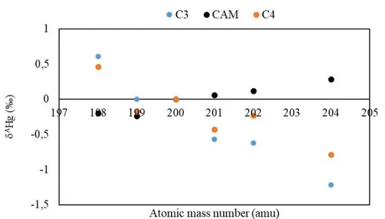
C3 and C4 type of plants are enriched in light isotopes and depleted in heavy isotopes and have small difference in magnitude of fractionation. On the other hand, the flower and the main body (SM-3-F and SM-3-L respectively) of one CAM plant are enriched in heavy isotopes and therefore different from the rest of the plant samples. There is big analytical uncertainty associated with sample SM-3 but the data appear to best indicate an absence of any isotope
fractionation effects relative to the standard. (Table 3 and Figure 1).
As mentioned in the sampling part, it was not possible to obtain roots of all the samples and low ion currents (<150-200 milivolts) caused inaccurate isotopic measurements for stems of the samples therefore it was not possible to report all parts of the plant samples. In general, the highest signal intensities were obtained from leaves following by roots. There is just one stem sample that ran well.
When different plant parts are compared (roots and leaves of C3 plants), it was observed that both leaves and roots are enriched in light isotopes and depleted in heavy isotopes but the roots show slightly higher fractionation than the leaves (Table 4 and figure 2).
Previous studies gave similar results. For example; (Yin et al., 2013) reported average 202Hg value of -3,28 ‰ for
rice plant which is much more depleted than the leaves used in this study (-0,61 ‰ for leaves of C3 plants). Similarly, 202Hg values reported to be around -2,0 to -2,6 ‰ for leaves of deciduous and coniferous trees (Demers, Blum, &
Zak, 2013; Jiskra et al., 2015; Yin et al., 2013). this negative 202Hg values observed is possibly due to photochemical
reduction and loss of Hg from the surface of the leaves (Yin et al., 2013). Indeed, other studies also showed MDF of even isotopes during biological processes such as photoreduction, methylation and volatilization.
Table 2. 13C Values of the Plant Samples
Taking all the samples and plant parts together, it can be said that even mass number isotopes indicate mass dependent fractionation while odd isotopes show mass independent fractionation. In all the measured samples, the delta values plotted against the respective isotope masses define a linear line. The odd isotopes deviate from this line and show negative anomaly. This deviation is expressed as 199Hg and 201Hg. In
other words, the degree of mass independent fractionation is indicated by 201Hg and 199Hg values and these are
calculated as follows (Eq.3);
ΔAHg = δAHg
measured – δAHgMDF (3)
where δAHg
MDF is calculated by using slope and interception of the mass dependent line.
In all the samples, 199Hg values range between -0,09 and -0,60 ‰ and 201Hg values are between 0,03‰ and -SAMPLE NUMBER 13 C (‰) PB1 -30.45 PB2 -15.28 PB3 -30.41 PB4 -28.22 PB5 -30.96 PB7 -30.02 PB9 -28.72 PB10 -30.22 PB11 -28.72 SM-1 -28.74 SM-2 -27.51 SM-3 -13.94 SM-4 -27.78 SM-6 -26.91 SM-7 -28.36 SM-8 -29.02 SM-9 -14.46
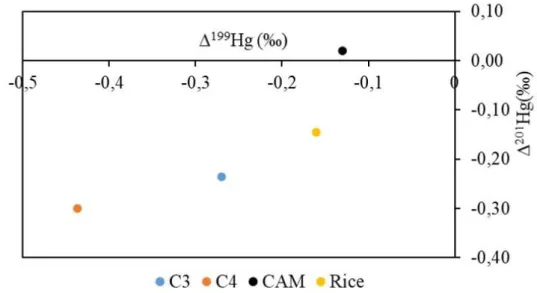
0,49 ‰ with average values being -0,28 and -0,22 respectively (Table 3). It is clear in the Figure 3 that C4 plants have the highest negative MIF degree (especially 199Hg) compared to C3 and CAM plants. In contrast, CAM plant
have slightly positive 201Hg deviation however considering the number of CAM plant samples (only 1) and the
analytical uncertainty associated with this sample, this interpretation is open to discussion. Taking these into consideration, it can still be suggest that the degree of MIF of odd Hg isotopes can be related to the photosynthetic type of plants. For comparison, Hg isotopic data of rice plants taken from Yin et al. (2013) were used, 199Hg and
201Hg values (average of leaves and roots) was plotted on the diagram (Figure 4). It is clear that rice plant, which is
also a C3 plant, plots close to C3 plant data point however they are not clustered.
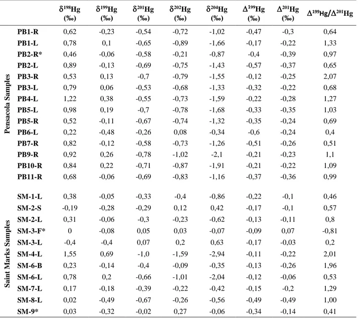
Table 3. AHg/200Hg Values (‰), 201Hg and 199Hg Values and Ratios of Different Parts of the Plants (L:
leaves, R:roots, S: stems, B: berries).
198Hg (‰)
199Hg (‰)
201Hg (‰)
202Hg (‰)
204Hg (‰)
199Hg (‰)
201Hg (‰)
199Hg/201Hg
P ens a co la Sa mp les PB1-R 0,62 -0,23 -0,54 -0,72 -1,02 -0,47 -0,3 0,64 PB1-L 0,78 0,1 -0,65 -0,89 -1,66 -0,17 -0,22 1,33 PB2-R* 0,46 -0,06 -0,58 -0,21 -0,87 -0,4 -0,39 0,97 PB2-L 0,89 -0,13 -0,69 -0,75 -1,43 -0,57 -0,37 0,65 PB3-R 0,53 0,13 -0,7 -0,79 -1,55 -0,12 -0,25 2,07 PB3-L 0,79 0,06 -0,53 -0,68 -1,33 -0,32 -0,22 0,68 PB4-L 1,22 0,38 -0,55 -0,73 -1,59 -0,22 -0,28 1,27 PB5-L 0,98 0,19 -0,7 -0,78 -1,68 -0,33 -0,35 1,03 PB5-R 0,52 -0,11 -0,67 -0,74 -1,32 -0,35 -0,24 0,69 PB6-L 0,22 -0,48 -0,26 0,08 -0,34 -0,6 -0,24 0,4 PB7-R 0,82 -0,12 -0,58 -0,73 -1,26 -0,51 -0,26 0,51 PB9-R 0,92 0,26 -0,78 -1,02 -2,1 -0,21 -0,23 1,1 PB10-R 0,84 0,22 -0,71 -0,87 -1,91 -0,21 -0,22 1,09 PB11-R 0,68 -0,06 -0,69 -0,83 -1,16 -0,37 -0,36 0,99 Sa int M a rks Sa m ples SM-1-L 0,38 -0,05 -0,33 -0,4 -0,86 -0,22 -0,1 0,46 SM-2-S -0,19 -0,28 -0,29 0,12 0,42 -0,17 -0,1 0,57 SM-2-L 0,31 -0,06 -0,3 -0,23 -0,62 -0,13 -0,11 0,8 SM-3-F* 0 -0,08 0,05 0,03 -0,07 -0,09 0,07 -0,81 SM-3-L -0,4 -0,4 0,07 0,2 0,63 -0,17 -0,03 0,2 SM-4-L 1,55 0,69 -1,0 -1,59 -2,94 -0,11 -0,22 2,01 SM-6-B 0,23 -0,14 -0,4 -0,09 -0,35 -0,13 -0,26 1,96 SM-6-L 0,78 0,2 -0,66 -1,01 -2,04 -0,12 -0,06 0,53 SM-7-L 0,17 -0,18 -0,39 -0,22 -0,42 -0,15 -0,2 1,29 SM-8-L 0,02 -0,49 -0,67 -0,26 -0,56 -0,49 -0,49 1,00 SM-9* 0,03 -0,32 -0,02 0,27 -0,06 -0,34 -0,14 0,41Figure 1.AHg (‰) vs Atomic Mass Number Plots of C3, C4 and CAM Plants
Table 4. Average AHg/200Hg values (‰), 201Hg and 199Hg values and ratios of All Samples, Pensacola
Samples, Saint Mark’s Samples, Different Parts of the Plants and of C3, C4 and CAM Plants 198Hg (‰)
199Hg (‰)
201Hg (‰)
202Hg (‰)
204Hg (‰)
199Hg (‰)
201Hg (‰)
Average all 0,53 -0,04 -0,50 -0,51 -1,04 -0,28 -0,22 Average C3 0,61 0,002 -0,57 -0,62 -1,21 -0,27 -0,24 Average C4 0,46 -0,17 -0,43 -0,23 -0,78 -0,44 -0,30 Average CAM -0,2 -0,24 0,06 0,12 0,28 -0,13 0,02Figure 3. Average 201Hg vs 199Hg Plots of C3, C4 and CAM Plants. Rice Plant (Leaves And Roots Average)
Results Are Taken From Yin et al. (2013)
Figure 4. Average 201Hg vs 199Hg Plots of C3 Plant Parts. Rice Plant Data are Taken from Yin et al. (2013)
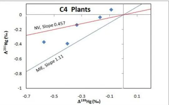
To understand the possible cause for MIF observed in plants, 201Hg/199Hg ratios produced by the effects of
magnetic isotope effect (MIE, blue lines) and nuclear volume (NV, red lines) were plotted on the 199Hg vs201Hg
diagram, with 201Hg/199Hg ratios of 1.11 and 0.457 respectively (S Ghosh et al., 2008). Figure 5 and 6 indicate
that MIF in these plant samples cannot be solely explained by either MIE or NV effect. A combination of both effects is likely responsible for the negative 201Hgandg values observed.
In addition, using MIF and NV effect lines it can also be suggested that MIF differences between roots and leaves (Figure 5) cannot be accounted for by either the NV or the MIE. The most simple explanation is that leaves and roots have acquired some of their mercury from different sources that already had been isotopically fractionated independent of their masses. In 2010, Ghosh found large differences between the 199Hg and 201Hg values of
epiphytes (negative deviations) and the atmosphere (~0 or slightly positive deviations) and suggested that MIF effects can be produced within plants (Ghosh, 2010). Therefore, the isotopic differences in root-leaf pairs found in this study may also be due to in vivo effects as well.
Figure 5. 199Hg vs 201Hg Plot for Pensacola Plant Samples (Blue Line 201Hg/ 199Hg =1.11, Red Line 201Hg/
Figure 6. 199Hg vs.201Hg Plot for C3 and C4 Plants (Blue Line 201Hg/ 199Hg =1.11, Red Line 201Hg/ 199Hg
=0.457). CONCLUSION
In the present study, Hg and C stable isotopic compositions of terrestrial plants were analyzed to understand if the Hg isotopic features of plants differ with different photosynthetic pathways and to understand the possible differences between above and below ground parts. Results showed that both C3 and C4 plants showed light Hg isotope enrichment, with mass dependent fractionation being approximately 3 times greater in the C3 plants than in C4 plants (-0.29‰/amu) compared to (-0.09‰/amu). The Hg isotopic signature of the single CAM plant is different than that of the C3 and C4 plants and showed light-isotope depletion. Together, these findings may suggest that there is a relationship between Hg isotopic composition in plants and their photosynthetic pathways.
Hg isotopic signatures of leaves and roots showed that both parts are enriched in light isotopes however roots fractionated slightly more than the leaves. In both parts of the plants odd isotopes of Hg showed negative MIF but the degree of MIF is different which cannot be explained only by known processes, if both roots and leaves obtain their mercury from same source. Considering the previous studies showing no MIF in atmospheric samples but negative MIF in leaves, it can be suggested that in vivo reactions in plants contribute to Hg isotopic fractionation in plants.
As a conclusion, this study provides an important step toward understanding biogeochemical cycle of Hg and improves our understanding of Hg isotope fractionation behavior in different plant types and in different organs of plants however there is a need for additional focused sampling and experiments on plants grown in controlled environment.
ACKNOWLEDGEMENT
This work was financially supported by the Ministry of National Education of Turkey. REFERENCES
Bergquist, B. A., & Blum, J. D. (2007). Mass-Dependent and -Independent Fractionation of Hg Isotopes by Photoreduction in Aquatic Systems. Science, 318(5849), 417 LP – 420. https://doi.org/10.1126/science.1148050 Biswas, A., Blum, J. D., Bergquist, B. A., Keeler, G. J., & Xie, Z. (2008). Natural mercury isotope variation in coal deposits and organic soils. Environmental Science and Technology, 42(22), 8303–8309. https://doi.org/10.1021/es801444b
Blum, J. D., Johnson, M. W., Gleason, J. D., Demers, J. D., Landis, M. S., & Krupa, S. (2012). Mercury Concentration and Isotopic Composition of Epiphytic Tree Lichens in the Athabasca Oil Sands Region. In K. E. B. T.-D. in E. S. Percy (Ed.), Alberta Oil Sands (Vol. 11, pp. 373–390). Elsevier. https://doi.org/https://doi.org/10.1016/B978-0-08-097760-7.00016-0
Cai, H., & Chen, J. (2016). Mass-independent fractionation of even mercury isotopes. Science Bulletin, 61(2), 116– 124. https://doi.org/10.1007/s11434-015-0968-8
Carignan, J., Estrade, N., Sonke, J. E., & Donard, O. F. X. (2009). Odd Isotope Deficits in Atmospheric Hg Measured in Lichens. Environmental Science & Technology, 43(15), 5660–5664. https://doi.org/10.1021/es900578v
Das, R., Salters, V. J. M., & Odom, A. L. (2009). A case for in vivo mass-independent fractionation of mercury isotopes in fish. Geochemistry, Geophysics, Geosystems, 10(11), 1–12. https://doi.org/10.1029/2009GC002617 Demers, J. D., Blum, J. D., & Zak, D. R. (2013). Mercury isotopes in a forested ecosystem: Implications for air-surface exchange dynamics and the global mercury cycle. Global Biogeochemical Cycles, 27(1), 222–238. https://doi.org/10.1002/gbc.20021
Donovan, P. M., Blum, J. D., Yee, D., Gehrke, G. E., & Singer, M. B. (2013). An isotopic record of mercury in San Francisco Bay sediment. Chemical Geology, 349–350, 87–98. https://doi.org/10.1016/j.chemgeo.2013.04.017 Driscoll, C. T., Mason, R. P., Chan, H. M., Jacob, D. J., & Pirrone, N. (2013). Mercury as a Global Pollutant: Sources, Pathways, and E ff ects. Environmental Science & Technology, 47, 4967–4983.
Durnford, D., Dastoor, A., Figueras-Nieto, D., & Ryjkov, A. (2010). Long range transport of mercury to the Arctic and across Canada. Atmospheric Chemistry and Physics, 10(13), 6063–6086. https://doi.org/10.5194/acp-10-6063-2010
Foucher, D., Hintelmann, H., Al, T. A., & MacQuarrie, K. T. (2013). Mercury isotope fractionation in waters and sediments of the Murray Brook mine watershed (New Brunswick, Canada): Tracing mercury contamination and transformation. Chemical Geology, 336, 87–95. https://doi.org/10.1016/j.chemgeo.2012.04.014
Gehrke, G. E., Blum, J. D., & Marvin-DiPasquale, M. (2011). Sources of mercury to San Francisco Bay surface sediment as revealed by mercury stable isotopes. Geochimica et Cosmochimica Acta, 75(3), 691–705. https://doi.org/10.1016/j.gca.2010.11.012
Ghosh, S, Xu, Y., Humayun, M., & Odom, L. (2008). Mass-independent fractionation of mercury isotopes in the environment. Geochemistry, Geophysics, Geosystems, 9(3), 1–10. https://doi.org/10.1029/2007GC001827 Ghosh, Sanghamitra, Schauble, E. A., Lacrampe Couloume, G., Blum, J. D., & Bergquist, B. A. (2013). Estimation of nuclear volume dependent fractionation of mercury isotopes in equilibrium liquid-vapor evaporation experiments. Chemical Geology, 336, 5–12. https://doi.org/10.1016/j.chemgeo.2012.01.008
Ghosh, Sulata. (2010). Itotopic Composition of Mercury in the Atmosphere.
Hintelmann, H., & Zheng, W. (2011, November 18). Tracking Geochemical Transformations and Transport of Mercury through Isotope Fractionation. Environmental Chemistry and Toxicology of Mercury. https://doi.org/doi:10.1002/9781118146644.ch9
Jiskra, M., Wiederhold, J. G., Skyllberg, U., Kronberg, R. M., Hajdas, I., & Kretzschmar, R. (2015). Mercury Deposition and Re-emission Pathways in Boreal Forest Soils Investigated with Hg Isotope Signatures. Environmental Science and Technology, 49(12), 7188–7196. https://doi.org/10.1021/acs.est.5b00742
Lamborg, C. H., Fitzgerald, W. F., Damman, A. W. H., Benoit, J. M., Balcom, P. H., & Engstrom, D. R. (2002). Modern and historic atmospheric mercury fluxes in both hemispheres: Global and regional mercury cycling implications. Global Biogeochemical Cycles, 16(4), 51-1-51–11. https://doi.org/10.1029/2001gb001847
Lindberg, S., Bullock, R., Ebinghaus, R., Engstrom, D., Feng, X., Fitzgerald, W., … Seigneur, C. (2007). A Synthesis of Progress and Uncertainties in Attributing the Sources of Mercury in Deposition. Source: Ambio, 36(1), 19–32.
Pirrone, N., Keeler, G. J., & Nriagu, J. O. (1996). Regional differences in worldwide emissions of mercury to the atmosphere. Atmospheric Environment, 30(17), 2981–2987. https://doi.org/10.1016/1352-2310(95)00498-X Schroeder, H. (1998). Atmospheric Mercury-An Overview. Atmospheric Environment, 32(5).
Yin, R., Feng, X., Li, X., Yu, B., & Du, B. (2014). Trends and advances in mercury stable isotopes as a geochemical tracer. Trends in Environmental Analytical Chemistry, 2, 1–10. https://doi.org/10.1016/j.teac.2014.03.001
Yin, R., Feng, X., & Meng, B. (2013). Stable Mercury Isotope Variation in Rice Plants (Oryza sativa L.) from the Wanshan Mercury Mining District, SW China. Environmental Science & Technology, 47(5), 2238–2245. https://doi.org/10.1021/es304302a
Yuan, S., Zhang, Y., Chen, J., Kang, S., Zhang, J., Feng, X., … Huang, Q. (2015). Large Variation of Mercury Isotope Composition During a Single Precipitation Event at Lhasa City, Tibetan Plateau, China. Procedia Earth and Planetary Science, 13, 282–286. https://doi.org/10.1016/j.proeps.2015.07.066
Zadnik, M. G., Specht, S., & Begemann, F. (1989). Revised isotopic composition of terrestrial mercury.
International Journal of Mass Spectrometry and Ion Processes, 89(1), 103–110.
https://doi.org/https://doi.org/10.1016/0168-1176(89)85035-9
Zheng, W., & Hintelmann, H. (2010). Nuclear Field Shift Effect in Isotope Fractionation of Mercury during Abiotic Reduction in the Absence of Light. The Journal of Physical Chemistry A, 114(12), 4238–4245. https://doi.org/10.1021/jp910353y
Zheng, W., Obrist, D., Weis, D., & Bergquist, B. A. (2016). Mercury isotope compositions across North American forests. Global Biogeochemical Cycles, 30(10), 1475–1492. https://doi.org/10.1002/2015GB005323