DETERMINATION OF POSITIONING ACCURACIES BY
USING FINGERPRINT LOCALISATION AND
ARTIFICIAL NEURAL NETWORKS
byHakan KOYUNCU*
Computer Engineering Department, Istanbul Gelisim University, Istanbul, Turkey Original scientific paper
https://doi.org/10.2298/TSCI180912334K
Fingerprint localisation technique is an effective positioning technique to deter-mine the object locations by using radio signal strength, values in indoors. The technique is subject to big positioning errors due to challenging environmental conditions. In this paper, initially, a fingerprint localisation technique is deployed by using classical k-nearest neighborhood method to determine the unknown ob-ject locations. Additionally, several artificial neural networks, are employed, using fingerprint data, such as single-layer feed forward neural network, multi-layer feed forward neural network, multi-layer back propagation neural network, general re-gression neural network, and deep neural network to determine the same unknown object locations. Fingerprint database is built by received signal strength indicator measurement signatures across the grid locations. The construction and the adapt-ed approach of different neural networks using the fingerprint data are describadapt-ed. The results of them are compared with the classical k-nearest neighborhood meth-od and it was found that deep neural network was the best neural network tech-nique providing the maximum positioning accuracies.
Key words: received signal strength indicator, k-nearest neighborhood, artificial neural networks, single-layer feed forward neural network, multi-layer feed forward neural network, multi-layer back propagation neural network, general regression neural network, deep neural network
Introduction
Indoor position detection is an important topic to detect the positions of unknown ob-jects [1, 2] in recent years. An ideal positioning should achieve an accurate position detection, a robust construction, fast training stage and a low price. It should give accurate positioning results under difficult environmental conditions where the received signal strength indicator (RSSI) propagation is affected by multipath components and signal noise.
Fingerprint localisation technique identifies the object location by relying on the RSSI recordings from a test region. The k number of closest RSSI values with respect to RSSI val-ues received at object location is selected in that region and their weighted mean value of their co-ordinates is taken as the object location. Fingerprinting localisation system has two stages: training stage and localisation stage [3, 4]. During the training stage, a database of RSSI values against grid co-ordinates across the test area is obtained and stored. In the localisation stage, this Authorʼs e-mail: [email protected]
database is used to locate the unknown object co-ordinates. One of the most popular algorithms to determine the object locations is the k-nearest neighbourhood (k-NN) algorithm [5]. The RSSI values received from unknown object co-ordinates are incorporated with the RSSI values in the fingerprint database through Euclidean signal distances in this technique. The co-ordinates which give the smallest Euclidean distances are employed to calculate the unknown object lo-cations [6].
Artificial neural networks (ANN), [7], are deployed on the fingerprint databases to predict the unknown object co-ordinates. There are several ANN techniques such as SFFNN, MFFNN [8], GRNN [9], MBPNN, [10], and DNN, [11], to calculate the unknown object po-sitions.
Presently, positioning accuracies of physical objects are calculated by using radio frequency (RF) waves in indoor areas and several neural network (NN) techniques. In this study an overview of NN techniques are employed. Similarly, these NN techniques can also be deployed in thermal sciences [12]. Thermal data of indoor environments can be measured with the help of wireless sensor nodes and used to calculate real time object locations by employing NN. Furthermore, static and dynamic thermal problems, dynamic thermal con-trol, prediction of thermal conductivity, and dynamic viscosity are a few examples of using NN [13].
Initially, fingerprint localisation method with k-NN is employed in this work and unknown object locations are determined. Previously mentioned NN techniques are also de-ployed to determine the same unknown object locations. Finally, positioning accuracies are calculated and compared among all these techniques to find the most accurate of them. Fingerprint localisation technique
Fingerprint theory
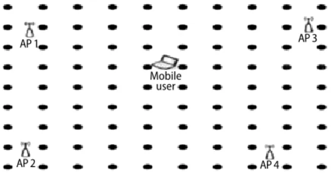
Fingerprint localisation technique determines the unknown object locations by using a set of RSSI values at object locations and comparing them with a pre-built RSSI fingerprint map. A general map of example fingerprint area is presented in fig. 1.
Measurement points in a grid formation depending on the area topology is orga-nized. The wirelles sensor networks (WSN) transmitters stationed at several points provide RF propagation over the entire grid area. During the training stage, RSSI values are received from all the transmitters at each grid point and recorded against the grid co-ordinates in a database.
The RSSI values at measure-ment points contain random be-haviour due to environmental con-ditions. Therefore, average value of multiple RSSI measurements is de-ployed as the RSSI fingerprint at that point. The RSSI measurement values are received at each grid point from
Ti transmitters. There are N number of transmitters. These measurement values are written in a database and Mobile user AP 1 AP 2 AP 3 AP 4
Figure 1. A test area of four transmitters, a grid of RSSI measurement points and a mobile receiver
defined as location fingerprint RSSI vector Fj.There are M number of grid points and Fj at jth grid point is given:
1, 2, 3,... N
j j j j
j T T T T
F =RSS RSS RSS RSS (1)
A sample of RSSI measurements are recorded on the object receiver and identified as
sample RSSI vector Rk. There are Z number of object points and Rk at kth object point is given:
1, 2, 3,... N
k k k k
k T T T T
R =RSS RSS RSS RSS (2)
The difference between the location fingerprint RSSI vector, Fj, and sample RSSI
vec-tor, Rk, are used to calculate the nearest grid points to the object point. Euclidean distance, Ek,
is identified as the signal distance and it is defined in eq. (3).
2 1( ) M k j k j E F R = =
∑
− (3)Euclidean distance defines the distance between two locations with respect to radio signal strengths. Therefore, weakest signal strength difference refers to the smallest physical distance between two locations [14]. Minimum Euclidean distances corresponding to minimum physical distance between grid and object locations are selected for object location calculations.
The k-NN algorithm
The k number of grid points are determined by k-NN algorithm in Euclidean database. Mean value of these grid co-ordinates are calculated to give the estimated object location.
Furthermore, a weighting scheme is introduced to increase the accuracy of object localisation with k-NN algorithm. Hence, weight functions, [15], are deployed to compensate the RSSI variations. Different weight functions can be utilized with respect to changing indoor conditions during positioning calculations.
Weights and distances are inversely proportional in many applications. Distant trans-mitters can have a dominant effect during localisation. Estimated positions move towards the nearest transmitter locations and the positioning errors increase. Finally, estimated object co-or-dinates are calculated by using weight function, wj, and grid co-ordinates, (xj, yj), defined by
k-NN algorithm, eq. (4). esti ted 1 ma ( , ) k j( , )j j j x y w x y = =
∑
(4)where wj is the weight function of the jth grid point in k-NN. The selection of weight functions effects the positioning accuracy. Hence wj is formulated to express this dependency with Dj Euclidean distances of k-NN values. Empirical weight function in eq. (5) is deployed in order to estimate the unknown object co-ordinates [16]:
2 2 1 1 1 j j k j j D w D = =
∑
(5)Artificial neural networks
The NN is a numerical modelling technique that mimics biological brains. A NN can initially be trained on a sample of known dataset. It determines the future similar patterns for unknown data which it has never seen before. The NN can change its structure depending on internal and external information during their flow through the network in training phase. The NN can be considered as non-statistical data modelling techniques [17, 18]. They are employed to show the relation between input and output data.
The feed-forward neural network
The FFNN is basically a straight forward network which relates the input and output functions [19]. In this technique, the signals travel through the network between input and output layers without any feedback. The performance of the NN is related to its input-output transfer function. Weights of the neurons reduce the errors between estimated and actual out-puts. Sigmoid function is employed for activation during the training stage to transfer the input data to output layer [20].
The FFNN consist of neurons which are constructed in layers. It generally has one input layer, one output layer. Neurons in the input layers are defined as input data and neurons in the output layer are defined as output data. Hidden layers, between the input and output layers, trans-form the input data to generate the target output data. The NN calculate the error derivative of the weights and back-propagation algorithm, [21], is the best method to derive these error derivatives.
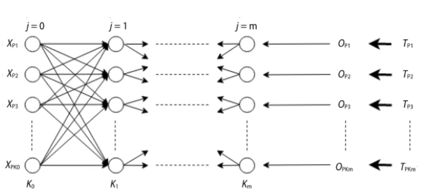
A description of the back-propagation multilayer network can be given in fig. 2. There are m layers in the multilayer network. The Kj is the number of neurons in jth layer. Network
has P number of patterns of training set with K0 dimensional X inputs. The Km dimensional
T targets are used in training of the network. The network O output response to the input and
target training patterns is given:
1, 2, 3... P P P PKm O O O O XP1 TP1 TP2 TP3 TPKm OP1 OP2 OP3 OPKm K0 K1 Km j = 0 j = 1 j = m XP2 XP3 XPK0
Figure 2. General feed forward and back propagation NN
Finally, different NN techniques are employed, and the most accurate technique is determined. Firstly, SFFNN technique is used. Its NN structures is shown in fig. 3. The neurons in the input and output layers represent the input and output data, respectively. The hidden layer between input and output layer carries out the transformation of input data to generate the target output data.
Target output data is the (x, y) position co-ordinates of grid points across the test area. There are j fingerprint signatures which are defined as the RSSI values received from j
transmit-ters at each grid location. Each neuron in a layer is con-nected to all the neurons in the next layer. Each of these connections is related by its weight, k
ij
w , where index i is the neuron number of the (k – 1) layer and j is the neuron number of kth layers. The output value of a neuron is mul-tiplied by the related weight and added to the signal value of the neuron in the next layer. Generally, the number of neurons in hidden layer is less than or equal to the size of the input layer and more than the size of the output layer. In this study, the size of hidden layer is taken as equal to the size of input layer as shown in fig. 3. Discrete
back-propagation algorithm can be applied to SFFNN if required. It is deployed to determine the weights and adjust them for each neuron in the hidden layer. This is a supervised learning method. The weights are adjusted several times in each epoch during the training.
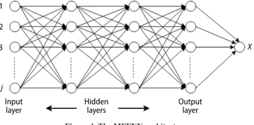
Secondly, MFFNN, multi-layer feed-forward artificial neural network technique is deployed. It includes one input layer, one output layer and several hidden layers as shown in fig. 4. The MFFNN technique is like SFFNN with the exception that the number of hidden layers is more than 1.
Figure 3. The SFFNN architecture
Input Hidden Output
j 3 2 1
Figure 4. The MFFNN architecture
j
3 2 1
Input
layer Hiddenlayers Outputlayer
X
Thirdly, back propagation method, MBPNN, can also be employed between hidden layers. This is identified as multiple back propagation neural network technique.
The ith neuron output in kth layer in the network can be determined:
1 1 1 (nk ) k k k k i ij i i i y g − w y − T = =
∑
+ (6)where g is the sigmoid activation function. It is used to model the non-linear relationship be-tween input and output layers. The k
i
T is the threshold value added to the input.
The MBPNN is used to calculate the final weights of neurons in the network. The error, calculated in the output layer neurons, is than back propagated to hidden layers by de-ploying the Gradient Descent method [22]. This minimizes the squared-error cost function in neurons. The sum of the squared-errors of cost function is given:
2 1 1 ( ) 2 m p kp kp k E h O = =
∑
− (7)where p is the number of training pattern, O – the actual output, and h – the predicted value with size m.
Similarly, j number of RSSI signatures is collected from j number of transmitters at each grid point. These signatures are employed as the input to the training network. The outputs of the network are defined as the (x, y) co-ordinates of the grid points and they are used as the two tar-gets during the training. Once the training phase is completed, any j numbers of RSSI signatures received from an unknown object location are applied as input to MFFNN and the output (x, y) co-ordinates are calculated. The prediction errors between the actual object co-ordinates and the calculated object co-ordinates are determined with different ANN techniques. Average error cal-culations between the ANN techniques are carried out to find the most accurate technique.
The general regression neural network
The GRNN has a one pass learning algorithm, [23]. The regression equation is con-sidered a parallel NN like structure. If the joint probability density function (pdf) of x and y is known and z co-ordinate is omitted, the conditional pdf and the expected value can be computed. Parameters of structures can be determined from examples rather than iteratively. The structure learns and starts to generalize. It can estimate y values for any new x value during the propaga-tion time. Suppose that f(x, y) represents the joint continuous pdf of a vector random variable x and scalar random variable y. The regression of y on x or conditional mean of y given x is defined:
( , ) ( ) ( , ) d d yf x y y R y x y f x y y ∞ −∞ ∞ −∞ =
∫
∫
(8)When f x y( , ) is unknown, it can be estimated from a sample of x and y data. A class of consistent estimators is proposed by Parzen, in [24], which can be applicable in the multi-di-mensional case. The probability estimator f x y( , ) is based on sample values of xi and yi of random variables of x and y and can be estimated from the training set by using the Parzen es-timator: 2 ( 1)/2 ( 1) 2 2 1 1 1 ( ) ( ) ( ) ( , ) exp exp (2 ) 2 2 i T i i n p p i x x x x y y f x y n σ σ σ + + = − − − = − − π
∑
(9)where n is the number of sample observations and p is the dimension of the vector variable x. The f x y( , ) assigns a sample probability of width σ for each sample of xi and yi. Probability estimate becomes the total sum of these sample probabilities. Placing the joint probability esti-mate f x y( , ) into conditional mean in eq. (8) generates the desired conditional mean y for giv-en x, eq. (10): 2 2 2 1 2 2 2 1 ( ) ( ) ( ) exp exp 2 2 ( ) ( ) ( ) ( ) exp exp 2 2 d d i T i i n i i T i i n i x x x x y y y y y x x x x x y y y σ σ σ σ ∞ = −∞ ∞ = −∞ − − − − = − − − −
∑
∫
∑
∫
(10)The term (x x− i T) (x x− i) in eq. (10) can be defined as a scalar function, 2 i
w , and eq. (10) becomes:
2 2 1 2 2 1 exp 2 ( ) exp 2 n i i i n i i w y y x w σ σ = = − = −
∑
∑
(11)The resulting regression in eq. (11) deals with the summations of the observations. The estimate y(x) can be considered as the weighted average of observed values, yi. Each ob-served value is exponentially weighted according to its Euclidean distance from x.
The deep neural network
A DNN, is an ANN with multiple hidden layers between input and output layers, [25]. The DNN is a feed forward network. Data flows from input layer to output layer without looping back. Deep learning methods target at learning feature hierarchies by using features from higher level hierarchy formed by the lower level features. They have learning methods of deep architec-tures with NN of many hidden layers.
There are two important issues with training DNN. These are overfitting and com-putation time. Overfitting takes place due to added layers of abstraction which allow to model simple dependences in the training data. Large number of data is used in DNN and computation time is longer compared to shallow ANN. The DNN use training parameters such as network size, learning rate and initial weights.
The most important advantage of deep learning is replacing handmade features with efficient algorithms for unsupervised or semi‐supervised feature learning and hierarchical fea-ture extraction. In this study 20 hidden layers with one input and one output layers are em-ployed for DNN. Similarly, RSSI values received at grid points are used as the inputs and the grid point co-ordinates are the outputs of the NN for training. Neural Designer software is deployed for DNN work.
Experiments
Fingerprint localisation
Fingerprint dataset which are used in this study is recorded in a sports hall with di-mensions of 20 meters by 10 meters and a grid space of 1 meter. Eight RFCODE manufactured wireless sensor nodes are used as transmitters at the corners and the boundaries of the hall. An RFCODE wireless sensor receiver is employed to collect RSSI data by placing it at each grid point during training stage.
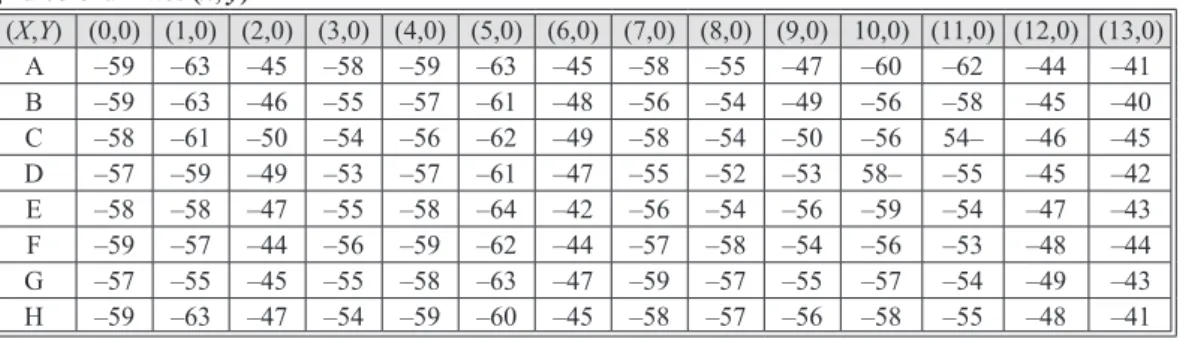
The collection of 8 RSSI values in dB form at each grid point is recorded in a dataset identified as fingerprint map in a server computer. There are total 200 fingerprint points and 1600 single recordings of RSSI values in the fingerprint map. Fingerprint map is extended by obtaining 100 sets of eight RSSI recordings totalling 800 RSSI values at each grid point. Hence, fingerprint map contains 160000 RSSI values. A sample data set of single RSSI values with respect to (x, y) grid co-ordinates are presented for the reader in tab. 1. Similarly, 800 RSSI val-ues received at each unknown object location are also recorded across the test area as the target RSSI values during localisation stage. They are used to calculate the unknown object location co-ordinates by deploying the trained NN.
Initially, classical fingerprint localisation technique is employed by using Euclidean distances between RSSI values at grid points and unknown object points. The k number of minimum Euclidean distances are selected by using k-NN algorithm. Weighting mechanism in
eq. (6) is applied with the grid co-ordinates corresponding to k number of Euclidean distances. Finally, eq. (5) is used to determine the final unknown object location co-ordinates. Error dis-tance values are calculated between the actual and the estimated object co-ordinates. A sample of k-NN localisation results is tabulated in tab. 2. Average error distance with k-NN localisation is approximately equal to 1 grid space.
Table 1. A sample of recorded single RSSI values in decibel form from eight transmitters against grid co-ordinates (x, y) (X,Y) (0,0) (1,0) (2,0) (3,0) (4,0) (5,0) (6,0) (7,0) (8,0) (9,0) 10,0) (11,0) (12,0) (13,0) A –59 –63 –45 –58 –59 –63 –45 –58 –55 –47 –60 –62 –44 –41 B –59 –63 –46 –55 –57 –61 –48 –56 –54 –49 –56 –58 –45 –40 C –58 –61 –50 –54 –56 –62 –49 –58 –54 –50 –56 54– –46 –45 D –57 –59 –49 –53 –57 –61 –47 –55 –52 –53 58– –55 –45 –42 E –58 –58 –47 –55 –58 –64 –42 –56 –54 –56 –59 –54 –47 –43 F –59 –57 –44 –56 –59 –62 –44 –57 –58 –54 –56 –53 –48 –44 G –57 –55 –45 –55 –58 –63 –47 –59 –57 –55 –57 –54 –49 –43 H –59 –63 –47 –54 –59 –60 –45 –58 –57 –56 –58 –55 –48 –41
Table 2. Samples of k-NN, SFFNN, and MFFNN localisation results
Unknown object
co-ordinates [m] k-NN estimated object co-ordinates [m] SFFNN estimated object co-ordinates [m] MFFNN estimated object co-ordinates [m]
X0 Y0 XE YE Error XE YE Error XE YE Error
2 2 2.9 2.8 1.20 2.7 2.7 0.99 2.6 2.5 0.78 2 8 2.8 8.7 1.06 2.6 8.5 0.78 2.5 8.7 0.86 3 4 3.7 4.9 1.14 3.5 4.5 0.71 3.6 4.4 0.72 5 7 5.8 7.7 1.06 5.4 7.6 0.72 5.5 7.4 0.64 6 3 6.7 3.8 1.06 6.5 3.6 0.78 6.4 3.7 0.81 8 5 8.9 5.9 1.27 8.6 5.6 0.85 8.6 5.5 0.78 12 3 12.7 3.6 0.92 12.5 3.6 0.78 12.6 3.7 0.92 14 8 14.8 8.7 1.06 14.6 8.5 0.78 14.5 8.6 0.78 16 5 16.9 5.5 1.02 16.6 5.9 1.08 16.4 5.9 0.98 18 7 18.6 7.9 1.08 18.5 7.7 0.86 18.6 7.5 0.78
Average error [m] 1.08 Average error [m] 0.83 Average error [m] 0.81
The SFFNN localisation
The SFFNN model is employed to determine the unknown object locations. The RSSI values arriving from eight transmitters are recorded at each grid point and stored in a database. There are 100 RSSI values coming from each transmitter resulting a total of 800 RSSI values at each grid point.
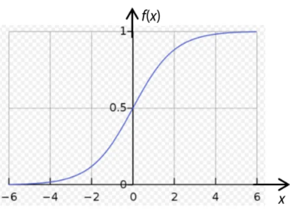
Hence these recordings for 200 grid points are used to train the NN. The NN is an adaptive network system. It can change its structure depending on external and internal infor-mation which flows through the network during the training phase. In SFFNN, the signals travel from input to output without any feedback [26]. Once the NN has been trained on samples of the known fingerprint database it will be able to predict the similar unknown patterns of fu-ture input RSSI data. The behaviour of the NN depends on the input-output transfer function. During the learning process, sigmoid activation function is employed to translate input signal to output signal, fig. 5.
Training model during learning pro-cess will have 100 sets of 8 RSSI data, 2 outputs of grid (x, y) co-ordinates and 1 hid-den layer of 8 neurons. Figure 3 displays the architecture of SFFNN. Once the NN train-ing is completed, 8 RSSI values received from unknown object location are applied at the inputs of the NN and the output co-or-dinates will be obtained as the target object co-ordinates.
The 100 sets of 8 RSSI values are ap-plied at the 8 inputs and 100 target co-ordi-nates are applied at the output of SFFNN. The network is trained with these values. In
localisation stage, 8 unknown RSSI values are applied to the input of the trained network. Un-known object co-ordinates of (x, y) is generated at the network output. A sample of results is tabulated in tab. 2.
The MFFNN localisation
The MFFNN model is similar to SFFNN with the exception that it has multiple hid-den layers between input and output layers, [27]. Input signal moves to output through sev-eral hidden layers. In this study 8 inputs, 5 hidden layers of 8 neurons each, and 2 outputs of (x, y) co-ordinates are deployed for MFFNN localisations. Similar training process is com-pleted where 100 sets of 8 RSSI values are applied as inputs and (x, y) co-ordinates of each grid point are given as 2 outputs. Input RSSI values passed through 5 hidden layers and ended at 2 outputs corresponding to grid co-ordinates. Same sigmoid activation function is used during the learning process to translate input signals to output signals. Eight RSSI values ar-riving from unknown object locations are applied to trained network inputs and target output co-ordinates are generated at the network outputs. A sample of MFFNN localisation results are given in tab. 2. It was observed that there is not much error distance difference between SFFNN and MFFNN.
The MBPNN localisation
The MBPNN is a combination of several NN models, [28]. It has multiple hidden layers between input and output layers. Feed-forward networks are straight forward network that relates the inputs and outputs. In order to make the NN suitable in specific tasks, the con-nections between neurons must be chosen carefully and the weights on the concon-nections must be selected properly. The signals, reaching to output layer, are back propagated to input layer. This forward and backward propagation between input and output layers several times helps to correct the weights between neurons. This way the error between the desired output and the real output will be reduced. The network must determine that how the error changes as the weight changes. Hence back propagation algorithm is the most widely used algorithm to calculate the error derivative of weights. Figure 2 illustrates the back-propagation model NN. Learning pro-cess is carried out similarly by training the network with input RSSI values and the output grid co-ordinates. The RSSI values arriving from unknown object location are applied as input and the output target co-ordinates are derived. A sample of MBPNN localisation results are given in tab 3.
Figure 5. Sigmoid activation function
x f(x)
The GRNN localisation
This localisation depends on the joint probability density function of x and y position co-ordinates given the RSSI training dataset [29]. Estimated value is the most probable value of y represented by eq. (8). Basic statistics of the input variables and the target variables which are used in eq. (10) are given in tab. 4.
The GRNN toolbox of MATLAB is used to gen-erate the GRNN model and carry out the training on input dataset. A sample of GRNN localisation results are presented in tab. 3.
The DNN localisation
In this study, DNN is considered as a feed-for-ward NN. It has large number of hidden layers, 20 of them, with 8 neurons each. The 1 input layer of 8 neurons and 1 output layers of 2 neurons are also ployed. Neural designer software has employed to de-termine the unknown object co-ordinates. A sample of DNN localisation results is presented in tab. 3. Results
Fingerprint database is built across a test area and it is used as training data for various NN models. This paper has presented a measurement and NN simulation-based localisation study. A summary of localisation accuracies is presented in tab. 5.
Initially classical weighted fingerprint localisation technique is implemented. Po-sitioning accuracy of a grid distance is calculated between the actual and estimated object positions.
There are 200 training points across the test area with 1 metre distances between them. Unknown object locations are estimated us-ing the learned network with these
Table 3. Samples of MBPNN, GRNN, and DNN localisation results
Unknown object
co-ordinates [m] MBPNN estimated object co-ordinates [m] GRNN estimated object co-ordinates [m] DNN estimated object co-ordinates [m]
X0 Y0 XE YE Error XE YE Error XE YE Error
2 2 2.4 2.5 0.64 2.4 2.6 0.72 2.4 2.4 0.57 2 8 2.5 8.6 0.78 2.4 8.4 0.56 2.5 8.4 0.64 3 4 3.6 4.5 0.78 3.5 4.5 0.70 3.5 4.4 0.64 5 7 5.4 7.6 0.72 5.4 7.5 0.64 5.4 7.4 0.57 6 3 6.4 3.5 0.64 6.4 3.5 0.64 6.3 3.5 0.58 8 5 8,5 5.4 0.64 8.4 5.5 0.64 8.3 5.5 0.58 12 3 12.5 3,6 0.78 12.4 3.4 0.57 12.2 3.5 0.54 14 8 14.5 8.4 0.64 14.4 8.5 0.64 14.3 8.5 0.58 16 5 16.4 5.7 0.81 16.5 5.5 0.70 16.3 5.4 0.5 18 7 18.5 7.4 0.64 18.4 7.6 0.72 18.3 7.5 0.58
Average error [m] 0.71 Average error [m] 0.65 Average error [m] 0.58
Table 4. Overall statistical values of input dataset for each transmitter across the fingerprint map
Tx/RSSI Min [dB] Max[dB] Mean [dB] Stdσ
A –92 –59 –60 4.64 B –90 –57 –61 4.59 C –94 –62 –65 4.37 D –91 –62 –65 4.32 E –96 –45 –52 7.17 F –94 –45 –49 6.90 G –90 –58 –62 7.21 H –88 –58 –62 7.11
Table 5. Summary of average localisation accuracies
Average localisation accuracies
k-NN SFFNN MFFNN MBPNN GRNN DNN
training points. There are 8 anchor points where the RF transmitters are located. As a result, there are 8 RSSI values recorded at each training grid point. In this study, large numbers of unknown object locations are tested to estimate their positions.
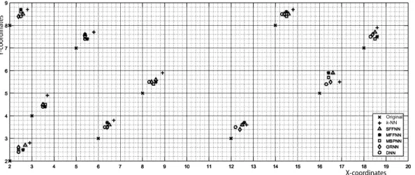
Overview of several NN models such as SFFNN, MFFNN, MBPNN, GRNN, and DNN are presented for the application of fingerprint localisation. Each model has generat-ed its own localisation accuracies. It was observgenerat-ed that as the number of hidden layers is increased the localisation accuracies are also increased. Graphical representation of target object co-ordinates and the estimated target object co-ordinates with different NN techniques are given in fig. 6.
Figure 6. Graphical view of sample target co-ordinates and estimated target co-ordinates with different NN techniques
X-coordinates Y-coor dina tes Original k-NN
The SFFNN and MFFNN models did not show large accuracy difference between them. On the other hand, MBPNN and GRNN models have displayed considerable localisation accuracy, around 30% more, compared to classical k-NN technique. The best NN model was found to be DNN model. Large number of hidden layers is employed in this model. The locali-sation accuracies with DNN model increased %50 relative to k-NN model.
The RSSI based NN simulations have shown that localisation accuracies are drastical-ly improved compared to classical k-NN technique. A fair size database of 200 points is suffi-cient enough to achieve good localisation accuracies. Future work will consist of advance DNN studies with different number of hidden layers and introduction of back propagation between these layers using different applications.
Acronyms
ANN – artificial neural networks DNN – deep neural network
GRNN – general regression neural network
k-NN – k-nearest neighborhood
MBPNN – multi-layer back propagation neural network
MFFNN – multi-layer feed forward neural network
NN – neural network
pdf – probability density function RF – radio frequency
RSSI – received signal strength indicator SFFNN – single-layer feed forward neural
network
References
[1] Bahl, P., Padmanabhan, V. N., Radar: an In-Building RF-Based User Location and Tracking System,
Proceedings, IEEE INFOCOM 2000 Conference on Computer Communications, 19th Annual Joint
Con-ference of the IEEE Computer and Communications Societies (Cat. No.00CH37064), Tel Aviv, Israel, 2000, Vol 2., pp. 775-784
[2] Ansari, J., et al., Combining Particle Filtering with Cricket System for Indoor Localization and Tracking Services, Proceedings, 2007 IEEE 18th International Symposium on Personal, Indoor and Mobile Radio
Communications, Athens, Greece, 2007, pp. 1-5
[3] Le Dortz, N., et al., WiFi Fingerprint Indoor Positioning System Using Probability Distribution Com-parison, Proceedings, 2012 IEEE International Conference on Acoustics, Speech and Signal Processing (ICASSP), Kyoto, Japan, 2012, pp. 2301-2304
[4] Wang, X., et al., PhaseFi: Phase Fingerprinting for Indoor Localization with a Deep Learning Approach,
Proceedings, 2015 IEEE Global Communications Conference (GLOBECOM), San Diego, Cal., USA,
2015, pp. 1-6
[5] Ilias, B., et al., Indoor Mobile Robot Localization Using KNN, Proceedings, 2016 6th IEEE International
Conference on Control System, Computing and Engineering (ICCSCE), Batu Ferringhi, Malaysia, 2016, pp. 211-216
[6] Gansemer, S., et al., RSSI-Based Euclidean Distance Algorithm for Indoor Positioning Adapted for the Use In Dynamically Changing WLAN Environments and Multi-Level Buildings, Proceedings, 2010 In-ternational Conference on Indoor Positioning and Indoor Navigation, Zurich, Switzerland, 2010, pp. 1-6 [7] Ibrahim, A., et al., Performance Evaluation of RSS-Based WSN Indoor Localization Scheme Using Ar-tificial Neural Network Schemes, Proceedings, 2015 IEEE 12th Malaysia International Conference on
Communications (MICC), Kuching, Malaysia, 2015, pp. 300-305
[8] Hayashi, Y., et al., Multi-Layer Versus Single-Layer Neural Networks and an Application to Reading Hand-Stamped Characters, Proceedings, International Neural Network Conference, Paris, 1990, Vol. 2, pp. 781-784
[9] Rahman, M. S., et al., RSS-Based Indoor Localization Algorithm for Wireless Sensor Network Using Generalized Regression Neural Network, Arabian Journal for Science and Engineering, 37 (2012), 4, pp 1043-1053
[10] Zbeda, R., Nathan, P., Multilayer Neural Network with Back Propagation: Hardware Solution to Learning XOR, Journal of Computing Sciences in Colleges, 20 (2005), 5, pp. 144-146
[11] Xiao, L., et al., A Deep Learning Approach to Fingerprinting Indoor Localization Solutions, 2017,
Pro-ceedings, 27th International Telecommunication Networks and Applications Conference (ITNAC),
Mel-bourne, Australia, 2017, pp. 1-7
[12] Yang, K., Artificial Neural Networks (ANN): A New Paradigm for Thermal Science and Engineering,
ASME J. Heat Transfer, 130 (2008), 9, pp. 093001-1-093001-19
[13] Esfe, M. H., et al., Designing an Artificial Neural Network to Predict Thermal Conductivity and Dynamic Viscosity of Ferromagnetic Nanofluid, International Communications in Heat and Mass Transfer, 68 (2015), Nov., pp. 50-57
[14] Halsted, T., Schwager, M., Distributed Multi-Robot Localization from Acoustic Pulses Using Euclidean Distance Geometry, Proceedings, 2017 International Symposium on Multi-Robot and Multi-Agent Sys-tems (MRS), Los Angeles, Cal., USA, 2017, pp. 104-111
[15] Peng, Y., et al., An Iterative Weighted KNN (IW-KNN) Based Indoor Localization Method in Bluetooth Low Energy (BLE) Environment, Proceedings, 2016 Intl IEEE Conferences on Ubiquitous Intelligence & Computing, Advanced and Trusted Computing, Scalable Computing and Communications, Cloud and Big Data Computing, Internet of People, and Smart World Congress (UIC/ATC/ScalCom/CBDCom/IoP/ SmartWorld), Toulouse, France, 2016, pp. 794-800
[16] Koyuncu, H., Yang, S. H., Comparison of Indoor Localization Techniques by Using Reference Nodes and Weighted k-NN Algorithms, Proceedings, 3rd European Conference of Computer Science (ECCS'12)
Recent Advances in Information Science, Paris, France, 2012, Vol. 8, pp. 46-51
[17] El Assaf, A., et al., Robust ANNs-Based WSN Localization in the Presence of Anisotropic Signal Atten-uation, IEEE Wireless Communications Letters, 5 (2016), 5, pp. 504-507
[18] Borenovic, M., Neskovic, A., ANN Based Models for Positioning in Indoor Wlan Environments,
[19] Zouari, R., et al., Indoor Localization Based on Feed-Forward Neural Networks and CIR Fingerprint-ing Techniques, ProceedFingerprint-ings, 2014 IEEE Radio and Wireless Symposium (RWS), Newport Beach, Cal., USA, 2014, pp. 271-273
[20] Murugadoss, R., Ramakrishnan, M., Universal Approximation of Nonlinear System Predictions in Sig-moid Activation Functions Using Artificial Neural Networks, Proceedings, 2014 IEEE International Con-ference on Computational Intelligence and Computing Research, Coimbatore, India, 2014, pp. 1-6 [21] Cruz-Lopez, J. A., et al., Training Many Neural Networks in Parallel via Back-Propagation, Proceedings,
2017 IEEE International Parallel and Distributed Processing Symposium Workshops (IPDPSW), Lake Buena Vista, Fla., USA, 2017, pp. 501-509
[22] Nayak, J., et al., A Hybrid PSO-GA based Pi Sigma Neural Network (PSNN) with Standard Back Propaga-tion Gradient Descent Learning for ClassificaPropaga-tion, Proceedings, 2014 InternaPropaga-tional Conference on Control, Instrumentation, Communication and Computational Technologies (ICCICCT), Kanyakumari, India, 2014, pp. 878-885
[23] Specht, D. F., A General Regression Neural Network, IEEE Transactions on Neural Networks, 2 (1991), 6, pp. 568-576
[24] Duin, R. P. W., On the Choice of Smoothing Parameters for Parzen Estimators of Probability Density Functions, in IEEE Transactions on Computers, C-25 (1976), 11, pp. 1175-1179
[25] Lee, N., Han, D., Magnetic Indoor Positioning System Using Deep Neural Network, Proceedings, 2017 International Conference on Indoor Positioning and Indoor Navigation (IPIN), Sapporo, Japan, 2017, pp. 1-8
[26] Wang, R., et al., Active Learning Based on Single-Hidden Layer Feed-Forward Neural Network,
Pro-ceedings, 2015 IEEE International Conference on Systems, Man, and Cybernetics, Kowloon, Hong Kong,
China, 2015, pp. 2158-2163
[27] Youssefi, B., et al., Efficient Mixed-Signal Synapse Multipliers for Multi-Layer Feed-Forward Neural Networks, Proceedings, 2016 IEEE 59th International Midwest Symposium on Circuits and Systems
(MWSCAS), Abu Dhabi, UAE, 2016, pp. 1-4
[28] Keller, J. M., et al., Multilayer Neural Networks and Backpropagation, in: Fundamentals of
Computa-tional Intelligence: Neural Networks, Fuzzy Systems, and Evolutionary Computation, The Institute of
Electrical and Electronics Engineers, Inc., Piscataway, N. J., USA, 2016, Chaper 3, pp.35-60
[29] Cui, H., Tu, N., Generalized Regression Neural Networks Based HVDC Transmission Line Fault Local-ization, Proceedings, 7th International Conference on Intelligent Human-Machine Systems and
Cybernet-ics, Hangzhou, China, 2015, pp. 25-29
Paper submitted: September 12, 2018 Paper revised: October 30, 2018 Paper accepted: November 16, 2018
© 2019 Society of Thermal Engineers of Serbia Published by the Vinča Institute of Nuclear Sciences, Belgrade, Serbia. This is an open access article distributed under the CC BY-NC-ND 4.0 terms and conditions