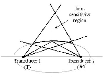
A simulation model of indoor environments for ultrasonic sensors
Tam metin
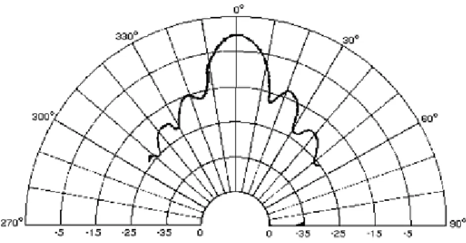
Şekil

Benzer Belgeler
architectural design (traditional media: paper-based drawings and physical scale models; and digital media) are analyzed in terms of their capacity to support dynamic
Mikro Kredi Kurumları’nın (MKK) maliyet etkinlikleri ölçülerinin hesaplanmasında stokastik sınır analizi yöntemi uygulanmış, ikinci aşamada maliyet
İnt- rauterin büyüme kısıtlılığı (doğum ağırlığı <10. persentil) olan (n=15) bebeklerin %80.0’ında, perinatal asfiksi olgula- rının %75.0’ında erken
feature_ruling kapalı bir pasaj, çıkıntı veya girintiyi belirlemek için kullanılır, feature_sweep, bir düzlem profil ile bu profilin süpüreceği uzunlamasına bir yol ve bir
Thus, the Russian legislation, although it does not recognize the embryo (fetus) as an independent legal personality, still has legal norms ensuring the recognition and protection
Bi rinci bölümde, “cinsiyet, mesleki deneyim, mezun oldu ğu okul, hizmetiçi eğitime katılma durumu, geçirdikleri teftiş sayısı” ile ilgili kişisel bilgiler
Cet article se propose donc de mettre en lumière quelques difficultés rencontrées lors de la traduction de l’ouvrage cité et d’attirer parallèlement l’attention sur les
Ebla to Damascus: Art and Archaeology of Ancient Syria, (ed.) H. Weiss, Washington, DC, ss. Geç Tunç Çağı Ege Dünyası’nda Bakır ve Tunç. Slotta, EgeYayınları, Bochum,
