Pergamon PII: S0305--0548(97)00073--7 Printed in Great Britain 0305-0548/98 $19.00+0.00
A N E W L O W E R B O U N D I N G S C H E M E F O R T H E T O T A L W E I G H T E D T A R D I N E S S P R O B L E M
M. Selim Akturk~-:~ and M. Bayram Yildirim§
Department of Industrial Engineering, Bilkent University, 06533 Bilkent, Ankara, Turkey
(Received September 1996; in revised form August 1997)
Scope and Purpose---qn enumerative methods, such as branch and bound algorithms, reducing the number of alternatives for finding the optimal solution is a key issue. This is usually done both by developing efficient upper and lower bounding schemes and by utilizing dominance properties, which usually rely heavily on the Emmons' dominance rules, to restrict the search space. We propose a new dominance rule which takes its background from adjacent pairwise interchange method for the single machine total weighted tardiness problem with job dependent penalties. The proposed dominance rule covers and extends the Emmons' results by considering the time dependent orderings between each pair of jobs, so that tighter upper and lower bounds are found as a function of start time of this pair.
Abstract--We propose a new dominance rule that provides a sufficient condition for local optimality for the Ill'wiT,. problem. We prove that if any sequence violates the proposed dominance rule, then switching the violating jobs either lowers the total weighted tardiness or leaves it unchanged. Therefore, it can be used in reducing the number of alternatives for finding the optimal solution in any exact approach. We introduce an algorithm based on the dominance rule, which is compared to a number of competing approaches for a set of randomly generated problems. We also test the impact of the dominance rule on different lower bounding schemes. Our computational results over 30,000 problems indicate that the amount of improvement is statistically significant for both upper and lower bounding schemes. © 1998 Elsevier Science Ltd. All rights reserved
1. I N T R O D U C T I O N
As firms struggle to survive in an increasingly competitive environment, a greater emphasis needs to be placed on coordinating the priorities of the firms throughout the functional areas. Firms have a variety of customers some of which are more important than others. The importance of a customer can depend on a variety of factors as stated by Jensen et al. [6], such as the firm's length of relationship with the customer, how frequently they provide business to the fLrm, how much of the firm's capacity they fill with orders and the potential of a customer to provide orders in the future. In many applications, meeting due dates and avoiding delay penalties are the most important goals of scheduling. The costs of tardy deliveries, such as customer bad will, lost future sales and rush shipping costs, vary significantly over customers and orders, and the implied strategic weight should be reflected in job priority. The vast majority of the job shop scheduling literature is replete with rules that do not consider job tardiness penalty or customer importance information. The firm's strategic priorities thus require the information pertaining to customer importance be incorporated into its shop floor control decisions. In addition, in the presence of job tardiness penalties, it may not be enough to measure the shop floor performance by employing unweighted performance measures alone which treat each job in the shop as equally important. In this paper, we propose a new dominance rule for the single machine total weighted tardiness problem with job dependent penalties, and implement in upper and lower bounding schemes.
Lawler [7] shows that the total weighted tardiness problem, lll~wjT~, is strongly NP-hard and gives a pseudo polynomial algorithm for the total tardiness problem, IllY.T~. Various enumerative solution methods have been proposed for both the weighted and unweighted eases. Emmons [3] derives several dominance rules that restrict the search for an optimal solution to the IlIET~ problem. Emmons' rules are
1" To whom all correspondence should be addressed (email: [email protected]).
:~ M. Selim Akturk is Assistant Professur of Industrial Engineering at Bilkent University, Turkey. He holds a Ph.D. in Industrial Engineering from Lehigh University, U.S.A., and B.S.I.E. and M.S.I.E. from Middle East Technical University, Turkey. His current research interests include production scheduling, cellular manufacturing systems and advanced manufacturing technologies.
§ M. Bayram Yildirim is a research assistant in the Department of Industrial Engineering at Bilkent University, Turkey. He holds a B.S.I.E. from Busphorus University, Turkey and an M.S.I.E. from Bilkent University. His current research interests include production scheduling and applied optimization.
used in both branch and bound (B&B) and dynamic programming algorithm~ (Fisher [4] and Potts and Van Wasserthove [8,9]). Rirmooy Kan et al. [11] extended these results to the weighted tardiness problem. Rachamadugu [10] identifies a condition characterizing adjacent jobs in an optimal sequence for l[[]gw;T~. Chambers et al. [2] develop new heuristic dominance rules and a flexible decomposition heuristic. The exact approaches used in solving the weighted tardiness problem are tested by Abdul-Razaq et al. [l] and they use Emmons' dominance rules to form a precedence graph for finding upper and lower bounds. They show that the most promising lower bound both in quality and time consumption is the linear lower bound method by Potts and Van Wassenhove [8], which is obtained from Lagrangian relaxation of machine capacity constraints. Hoogeveen and Van de Velde [5] reformulate the problem by using slack variables and show that better Lagrangian lower bounds can be obtained.
Szwarc [ 12] proves the existence of a special ordering for the single machine earliness-tardiness (E/T) problem with job independent penalties where the arrangement of two adjacent jobs in an optimal schedule depends on their start time. Szwarc and Liu [13] present a two-stage decomposition mechanism to l[[EwiT~ problem when tardiness penalties are proportional to the processing times. The importance of a customer can depend on a variety of factors as stated above but it is important for manufacturing to reflect these priorities in the scheduling decisions. Therefore, we present a new dominance rule for the most general case of total weighted tardiness problem. The proposed rule covers and extends the Emmons' results and generalizations of Riunooy Kan et al. by considering the time dependent orderings between each pair of jobs.
Since the implicit enumerative algorithms may require considerable computer resources both in terms of computation times and memory, several heuristics and dispatching rules have been proposed. Vepsalainen and Morton [14] develop and test efficient dispatching rules for the weighted tardiness problem with specified due dates and delay penalties. The proposed dominance rule provides a sufficient condition for local optimality, and it generates schedules that cannot be improved by adjacent job interchanges. We also propose an algorithm to demonstrate how the proposed dominance rule can be used to improve a sequence given by a dispatching rule. We prove that if any sequence violates the proposed dominance rule, then switching the violating jobs either lowers the total weighted tardiness or leaves it unchanged.
The weighted tardiness problem is NP-hard and the lower bounds in the literature are either weak or not practical to use due to extensive computational requirements. As a result, the exact solution for a 50 job problem is a barrier that could not be passed. The linear lower bound of Potts and Van Wassenhove is rather a weak lower bound but it is found to be the most promising one by Abdul-Razaq et al. which contradicts the often heard conjecture that one should restrict the search tree as much as possible by using the sharpest possible bounds. The linear lower bound calculations are based on an initial sequence. We show that having a better upper bound value, which is close to optimal solution, improves the lower bound value obtained from the linear lower bound method.
The remainder of this paper is organized as follows. In the Section 2, we discuss the underlying assumptions and give a list of definitions used throughout the paper. We discuss the proposed dominance rule in Section 3 along with the transitivity properties in Section 4. The lower bounding scheme is described in Section 5. Computational analysis is reported in Section 6. Finally, some concluding remarks are provided in Section 7.
2. P R O B L E M D E F I N I T I O N A N D N O T A T I O N
The single machine total weighted tardiness problem, 1 [l~wiT~, may be stated as follows. Each ofn jobs (numbered 1 .... ,n) is to be processed without interruption on a single machine that can handle only one job at a time. All jobs become available for processing at time zero. Job i has an integer processing time pi, a due date d~ and has a positive weight w,.. For convenience the jobs are arranged in an EDD indexing
convention such that d~<dj or d~=dj thenpi<pj or di=dj andp~=pj then wi>-wj for all i and j, such that i<j. For a particular schedule the tardiness of job i, T~, is either zero (in case it is completed before its due date d~) or otherwise it equals the difference of its completion time and its due date. The problem can be formally stated as: find a schedule S that minimizes J(S)=E~w~T~. To introduce the dominance rule, consider schedules S~=QI/JQ2 and S2=Qt/iQ2, where Ql and Q2 are two disjoint subsequences of the remaining n - 2 jobs. Let t=Ek~Q~Ok be the completion time of Q~.
The following interchange function, Ao(t), is used to specify the new dominance properties, which gives the cost of interchanging adjacent jobs i andj whose processing starts at time t.
Then, Ao(t) =~(t) - go(t).
f
O fj(t) = ( t + p i + p j - d i ) . w i "~pj.w i{ °
go(t)= ( t + p i + p j - d ) ' w j - p : w j t<--di - (Pi + P), d i - (p~+p)<_t<_di-p~, di - Pi<-t, t<-dj - ~oi + pj), d j - (pi+p)<--t<--dj- pj, dj - pj<-t.Note that this cost Ao(t) does not depend on how the jobs are arranged in QI and
Q2
but depends on start time t of the pair, and• if Ao(t ) < 0 then, j should precede i at time t; • if A0(t)>0 then, i should precedej at time t; • if A0(t)=0, it is indifferent to schedule i o r j first. Throughout the paper, we also use the following definitions:
• A breakpoint is a critical start time for each pair of adjacent jobs after which the ordering changes direction such that if t<-breakpoint, i precedesj (orj precedes i) and thenj precedes i (or i precedes
j).
• An ordering relation R between two jobs is transitive whenever iRj a n d j R k implies iRk.
• i globally precedes j, i ~ j , (j globally precedes i, j ~ i ) if it implies the existence of an optimal sequence in which job i (job j) precedes j o b j (job i) is guaranteed and the transitivity property holds such that if i ~ j a n d j ~ k then i ~ k .
• i unconditionally precedes j, (i--*j) the ordering does not change, i.e. i always precedesj when they are adjacent, but the transitivity property might not hold. Thus it does not imply that an optimal sequence exists in which i precedesj.
• i conditionally precedes j, (i<j) if there is at least one breakpoint between the pair of jobs then the order of jobs depends on the start time of this pair and changes in two sides of that breakpoint.
3. DOMINANCE RULE
Potts and Van Wassenhove [8] have verified the effectiveness of adjacent pairwise interchange (API) method as a pruning device in their B&B algorithm for the lllXw:, problem. The total weighted tardiness function is not convex so that API method can lead only to local improvements. However, the API method preceded by a good heuristic has a reasonable chance to lead to an optimal solution. Furthermore, if any sequence violates the proposed dominance rule, then switching the violating jobs either lowers the total weighted tardiness or leaves it unchanged. The proposed rule provides a sufficient condition for local optimality, and it generates schedules that cannot be improved by adjacent job interchanges.
When all of the possible cases are studied, it can be seen that there are at most three possible breakpoints for the lllXw~T~ problem as shown below:
t~=
w ~ l , - w f l jfP~+P),
(I)
W i - - W j
t~ = dj - Pi - P,( I - w/wj),
(2)
t~ =di - pj - pi(1 - w / w i ) . (3)
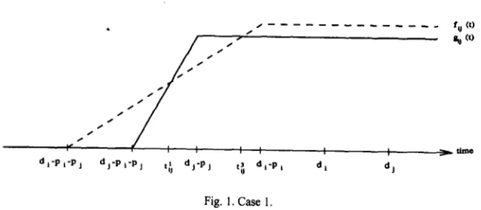
These breakpoints may be determined by looking at the points where the piecewise linear and continuous functions~(t) and go(O intersect. Assuming the EDD indexing convention in the sequel, the following six cases are exhaustive.
Case 1. di<dj, piw:<pjwi, p,(wj - w/) > (dj - d3wi. Case 2. di=dj, wi<wj, p~wj<pjwi.
Case 3. di<d j, piwj>pjw,, p~(wj - wt) > (d: - di)wy. Case 4. d~-<dj, p i ~ <-pjw,, p,(wj - w~)<_(dj - di)wi. Case 5. di=dh piwy>-pjwi.
/ J I~ I I I I I I d l ' P t ' P ] d J ' P I ' P J t~j d j - p j tg d l ' P l d | dj fu (t) i~ it) Fig. I. Case 1. C a s e 6. d~< dj, p,wj>pjw,, pj(wj - w~)<(~. - d~)wj.
In order to explain the new dominance rule, we will investigate how the interchange function Ao(t ) changes for each case. As a result, three breakpoints are found and transitivity properties are shown for certain instances.
3.1. ~ s e l
In this case, we have the two breakpoints t~ and t~ as it can be seen from Fig. 1. The following proposition can be used to specify the order of jobs at time t for this case.
P r o p o s i t i o n 1. l f d~< dj, piwj < pjw~ and p,(wj - w~) > (4" - d~)wi then there are two breakpoints t ~. and t 3, and for t<-t~, i<j, for t~<-t<-t3,j<i and for t>-t 3,
i<j.
Proof. If (t<-d~-(pi+pj)) then no tardiness occurs, so it is indifferent to schedule either i o r j first. If (d~- ( p i + p j ) < t < d j - (p,.+pj)), then i is tardy if not scheduled first. Here, Ao(t)=w~t+p~+pj- d). Since d~ - (pt+pj)< t, A0(t) >0 so i<j. If(dj - (p~+pj)<t<_dj-pj), then either i o rj is tardy if not scheduled first. Here, Ao(t)=(w i - wj)t+(pi+Pj)(w i - wj) -- w~di+w.td j. The breakpoint tb=[{(w,di - w ~ ) / ( w , - wj)}
- (p~+pj)] is defined in this region. If the processing of this pair starts up to t<-t~ then i<j andj<i if the processing begins after t~. If (dj-pj<<-t < di-p~), then j is always tardy but i is not tardy if scheduled first. Here, A~O=(t+p~+pj- d)w~-p~wj. There is an another breakpoint t~=di - p j - p ~ l - wfw~), a n d j < i for
t<--t~, i'<j
afterwards. If (dt-p~-<0 both jobs are tardy. Here,Ao(t)=Pjwi--PtW j. If A#(t)>O
then i<j,otherwise j<i. Moreover, from (3), we know that if t3 <di - p i then piwi<pjwi, which means A#(t) >0, so i<j. •
3.2. Case2
The second case can be considered as a special case of the first one such that di=dj=d as depicted in Fig. 2. In this case, t ~ = d - (pi+pi), therefore we are indifferent to schedule either job i or j o b j first up to t~.. Since d~=d~, p~<-_pj by the EDD ordering convention. Therefore, there can be a breakpoint if wt<wj as stated below.
Proposition 2. f f di =d J, wi<w j and piwj<pjw i then there is the breakpoint t~. I f the processing of this pair starts up to t<-t~ then j < i and i<j if the processing begins after t~.
d-p [-pj d-pj
fo (t)
"" g 0 (0
t~ d-p!
i dt-P t-P j j. s l dfp f p ) tl ~ dj-pj d f p t gu (t) ftl (t) time Fig. 3. Case 3. 3.3. Case3
This case is similar to the first case except, p~w/>--p/wi, hence there is only one breakpoint t~ as shown in Fig. 3.
Proposition 3. l f di<d :, PiWj>-p/w~ and pj(wj - wi)>(d j - di)w j then there is the breakpoint t~, and •<j for t<-t~, and j<• afterwards.
Proof. In this case we have to make sure that the nonconstant segments of~(t) and go(t) intersect, and the breakpoint t~ satisfies t~.=[(w:li-wfly(wi-wj)]-(p~+p/)<di-p, It leads to the condition of p:(wj - w~)> (d: - d,)w/, since Ao(t)=p/w , -p,w/<-O for t>-d~-p,. •
3.4. ~ s e 4
In this case, if we can show that i<j for every t then i---,j, that means Ao(t)>-O Vt, i.e.~(t)>-go(t ) Vt, as shown in Fig. 4.
Proposition 4. If di<-d/, p~w/<-p/wi and p,(w/- wi)<-(d: - di)wi then job i unconditionally precedes job j, i.e. (i---~j).
Proof. As defined earlier Ao(t)=~(0 -go(t). If we let t= d: - (p,
+p/)then 40(4
- p , - p / ) = (a/- di)wi>--O, since dg---di and go(d/-pt-p/)=0, so i<j at time dj - (p,+p/). Let t = d j - p / t h e n do(d :-p/)=(dg+pi - d~) w~ -p~w/=(d: - d~)w~ - p , ( w / - wi)>-O, since p,(w/- w.J<-(d: - d~)w~, so i<j at time d: - p j . If we let t=d~ -Pi then Ao(d~-p~)=p/we-piw/>-O, since p~w/<<-p/w~, consequently i<j again at time d ; - p , Therefore, the result follows and i--~j. •3.5. Case5
In the fifth case, di=dj=d as shown in Fig. 5, consequently p i - p j by the EDD ordering convention, that means wj>-wi in order to satisfy the ptwj>-pjwi condition. As discussed in the second case, t~=d- (pj+pj) when d~=d:, hence we are indifferent to schedule either job i or j o b j first up to t~.. If we can show that A~:(t)<-O Vt, that m e a n s j < i for every t, then j---.• as stated below.
Proposition 5. If d~=d: and p~wj>-pjw~ then job j unconditionally precedes job i, i.e. (/---.i).
Proof. Let t = d - p j then Ao(d-pj)=piwg-piwj=p,(wi-wj)<-O, since w/>-w, If we let t=d-p~ then A~:(d-pi)=p/w~-p~wj<-O. Therefore, Ao(t)~O Vt and j-.•. •
~. . . fij (t) 1 I I I j 1 1 1 1 1 1 ~ I / I I I d ~ ~ j dfp fp j dfp j dfp g~(t) m time Fig. 4. Case 4.
gtj (t) f i~ (t) . s . s s j , j . j , d-p i-p i d-p I d-p t Fig. 5. Case 5. 3.6. ~ s e 6
The sixth case is similar to Case 3 except dr-pr<d:-pj as shown in Fig. 6, although the relative positions of di-Pi and dj-(p;+p:.) might change such that if d : - di<-p: then d : - (pr+pj)<<-dr-Pr,
otherwise dr - p i > dj - (Pr + Pg).
Proposition 6. l f dr<d:, pr~>pjwj and pj(w: - wr)<-(d:- dr)wj then there is the brealepoint
t~, and
i<j for t<-t 2, and j < i afterwards.Proof. In order to have the breakpoint t 2 we have to make sure that the noneonstant segment ofgo(t ) intersects with the constant segment of~(t). This is the case if the breakpoint t~ with (t2+pr+pj- ~.)=pjwi
satisfies dr -p,<-t2.<d: - Pj. It leads to the conditions of prw:>pjwr for t~<dj- pj and pj(wj - wr)<-(d j - dr)wj
for t2>-dr-p, If (d:-pj<-t) t h e n j < i since Ao(t)=pjw r-prwj<O. •
After analyzing all of the possible cases, we prove that there are certain time points, called breakpoints, in which the ordering might change for adjacent jobs. We find three such breakpoints and show that there are at most two breakpoints, which are tb and t 3 in Case 1. Furthermore, there is exactly one breakpoint in Cases 2, 3 and 6, which are t~, 3 tq and tu, respectively. We do not have any breakpoint in Cases 4 and 2 5. As a result, we can state the following general rule, which provides a sufficient condition for local optimality, by using all of the properties of the dominance rule.
General rule IF dr=4 THEN IF prwj>-pjwr THEN j==*i ELSE IF wr-->wj THEN i='*j E L S E j < i for t<=t~. i<j for t>--t~ ELSE IF p,(w: - wr) > (d: - d,)wr
THEN i<j for t<--t~
IF pr~ >pyw,Apj(wj -- wr)> (d: - at)w:
J
I I I t dt'P rP } dj-p t'P ) d;-p I ~ t dj~pj U g u (¢) f o ( t ) t l r a ~ Fig. 6. Case 6.T H E N j < i for
t>-t~
E L S E j < i for
t~<--t<-t 3
i<j
fort>--t 3
ELSE IF
piwj<-pjwi
THEN
i---,j
ELSE
i<j
fort<--t~
j<i
fort>-t 2
Let Z denote the set of all jobs, C the set of pairs (ij) for which
Ao(t )
has at least one breakpointto,
id" ~ C, the largest of these breakpoints, and
t c
= max {t o. I (i j ) E C}. The following lemma can be used quite effectively to find an optimal sequence for the remaining jobs on hand after a time pointtc.
Lemma 1.
l f t> tc then the weighted shortest processing time (WSPT) rule gives an optimal sequence for
the remaining unscheduled jobs.
Proof. The tc
is the last breakpoint for any pair of jobsid
on the time scale. Furthermore, it is a well- known result that the WSPT rule gives an optimal sequence for the IlIEw;T~ problem when either all due dates are zero or all jobs are tardy, i.e.t>maxt~z{d~-pt }. The
problem reduces to total weighted completion time problem, which is known to be solved optimally by the WSPT rule, in which jobs are sequenced in non increasing order ofw/p~.
We know thattc<max~z{d ~-p~},
so we enlarge the region for which the total weighted tardiness problem can be solved optimally by the WSPT rule. We already show that for every job pair(ij),
one of these conditions must hold either there is a breakpoint or unconditional ordering(i---*j)
or globally precedence(i=*j).
The WSPT rule holds for bothi--*j and i~j.
If there is a breakpoint then for
t>t¢ the
job having higherw/p~
is scheduled first, so WSPT again holds. Fort>tc,
consider a job i which conflicts with the WSPT rule, then we can have a better schedule by making adjacent job interchanges which either lowers the total weighted tardiness value or leaves it unchanged. If we do same thing for all of the remaining jobs, we get the WSPT sequence. •4. T R A N S I T I V I T Y
The transitivity property is very crucial for reducing the number of sequences that have to be considered in an implicit enumeration technique. Szwarc [12] shows that there is a transitivity property for the IlI~T,- problem. The transitivity property does not hold for the lll~wiT~ problem even for the assumption that the weights are proportional to processing times as shown by Szwarc and Liu [13]. Therefore, we will present two possible cases in which transitivity property holds for the proposed dominance rule. Let
A~o(t)
is the cost of interchanging two jobs i a n d j whose processing starts at time t, and they are not necessarily adjacent and are separated by the subsequenee Q. Notice that when Q=Q,Aio(t)
reduces toAo(t).
Furthermore, T,.~(t) andTo(t ) are the
total weighted tardiness of all jobs in sets {iQ]} and {Q} respectively if their processing starts at time t,AiQi( t ) = TjQi( t ) - Tio3( t )
=wjmax(O,t+pj-dj)+ TQ(t+pj)+wimax(O,t+pj+ k~Qpk+pi--di)
- w , max(O,t+p,-d,)- TQ(t+p,)-wjmax(O,t+p,+ ,~Qp,+pj-dj).
L e m m a 2.
If di<-dj, pi<<-pj and wt>-wj then job i globally precedes job j, i.e. i=*j.
Proof.
It has been already proved by Rinnooy Karlet al.
[11]. •Lemma 3.
If di<dj, pi>pl and wi< w j then job j globally precedesjob i (]~i) for t> tiy.
Proof.
The breakpointt o.
can be either t~ or t~ from Cases 3 or 6, respectively, since the breakpoint t 3 can only occur whenptwj <pjw I
as shown in Cases 1 and 2. We have three possibilities to examine such as either both jobs can be tardy, that means there is not any breakpoint, or t~ is the only breakpoint from Case 3 or t~ is the only breakpoint from Case 6. We have already shown that both of these breakpointscannot occur at the same time for these cases. For provingj globally precedes i when both of the jobs are tardy 0"~/), we have to show that inserting a set of jobs Q betweenj and i does not alter the relative sequence o f j and i (i.e.j</) at a given time t > d j - p j . When both jobs are tardy, Ai~(t ) reduces to
Ai~(t ) = (w i -- wy) k~Q Pk + TQ(t+py) -- Ta(t+pi) + W.~y -- wfli.
Since w~-wj<O, p y - p i < O ~ w . l J y - w j p i < O and To(t+pj)<TQ(t+p.~, therefore, dz~(t)<O which means j ~ i . We can extend this result to t > t 2. Now, we are in the region where i is always tardy butj is not tardy
if scheduled first. In this region,
= TQ(t +py) -- Ta(t +Pi) + k~¢2 Pg(Wi -- wy) + w.~y -- wj(t +Pi +Py -- dy). Given
t> t 2 for jobs i and j, suppose that job i is scheduled before job j. If i a n d j are adjacent jobs then we can make an interchange which either lowers the total weighted tardiness value or leaves it unchanged to have a better schedule. Now, let us look at the case where they are not adjacent. Since t>t2=dj - p ~ - p j ( l - w~ w y ) ~ t = ~ - p ~ - p j ( 1 - w/w~)+ e I and el>O. dioi(t) can be written as follows:
A,ai( t ) = To( t + py) - To( t + pi) + k~o Pl~(wi
--
Wj) + W~j-- wy( dj - Pi -
Pj( 1 -- W/Wy) + e 1 dt'pi + pj -- 4 )=To(t+p j) - TQ(t+pi)+ k~a Pk(Wi- Wy) - wj~l~-~O
Using the similar arguments as stated above, we can improve the current schedule by replacing the positions of jobs i and j, i . e . j ~ i . A similar proof can be done for the t>t~ case where i o r j will not be tardy if scheduled first but the other one will be tardy as follows:
AiQ](t)=TQ(t+py)+Wi(t+pi+ k~Qpk+Py--di) -- TQ(t+pi ) -- Wj(t+pi+ k~Qpk+py-- 4)>0
= Te( t + Py) - To( t + Pi) + ~Q Pk(W i - wy) + ( w i - wy)(Pi + py) + t(w i - wj) - w,d, + wily. Givent> t~, t= [(walt - w/ty)/(w i - wy)] - (pi +py)+ ~2 and ~2>-0. =A,os(t) = TQ(t +py) - TQ(t +Pi) + k~Q pk(wi -- Wy) + E2(Wi -- Wy)<0,
s o
j ~ i . •
We have proved that the dominance properties provide a sufficient condition for local optimality. Now, we will present an algorithm based upon the dominance rule that can be used to improve the total weighted tardiness criterion of any sequence by making necessary interchanges. The proposed heuristic takes into account all of the global, unconditional and conditional precedence relationships. Let seq[i] denote index of the job in the ith position in the given sequence. The algorithm can be summarized as follows:
Initialization:
Sort the jobs in EDD order.
Calculate the breakpoint matrix using the general rule.
Forward procedure:
For i= 1 to n - 1 do F o r j = i + 1 to n do
If i globally precedes j (orj=~i) and seq[i] > seq[/] (or seq[i] < seq[/]) then change the orderings of i andj.
Set k= 1 and t=O. While k<-n - l do begin Set i=seq[k] a n d j = s e q [ k + l]
If i<j then
If there is the breakpoint t 3, dj - P c - p j < t and t b <t<-t~.
then t=t-Ps~qtk-~1, change the orderings of i andj and k = k - 1
else if either there is t~. or t 2 and t> t o. then
t=t -- Ps~qtk-11, change the orderings o f / a n d j and k = k - 1
else t=t+p~ and k=k+ 1.
If i>j then
If there is the breakpoint t 3, dj - P t - p j < t and either t<t)i or t>t 3 then
t=t -Ps~qtk-~1, change the orderings o f / a n d j and k k = k - 1
else if either there is t)i or t 2 and t<-tji then
t=t-Ps~qtk-]l, change the orderings o f / a n d j and k = k - 1
else t=t+pi and k=k+ 1
end.
L e m m a 4. The algorithm has a time complexity of O(n3).
Proof. We first obtain an EDD order that takes a total of O(n log n) time. In order to calculate the breakpoint matrix that has n(n - 1)/2 entries, we check for global dominances, and the breakpoints tb, t 2 and t 3 in the worst case for every job pair (ij), which require a total of O(n 2) time. In the forward procedure, we first check for the global dominances so that total of n(n - 1)/2 comparisons are done which take a total of O(n 2) time. Furthermore, we have to make ETS511i=n(n- 1)/2 comparisons to determine the job in position 1, i.e. seq [1]. Similarly, for the job in position 2, we have to make E~__-12i=(n - 1)(n - 2)/2 comparisons. In order to determine the job for the kth position, we have to make
Y,7-1ki=(n - k ) ( n - k + 1)/2 comparisons which make a total of
.-1 i ( i - 1 ) l n ~ l [ i E _ i ] = l I ( n - 1 ) n ( 2 n - 1 ) n ( n - 1 ) l
i=l 2 2 i=l 2 6 2
comparisons or a total of O(n 3) time. Therefore, the algorithm takes a total of max[O(n log n), O(n 2),
O(n 3)] = O(n 3) time.
5. L O W E R B O U N D I N G S C H E M E
We now present two lower bounding approaches for the 111Y~wi
T,
problem both by exploiting the results discussed in the previous sections and by relaxing some of the constraints of the original problem.5.1. Lower bound 1
The Emmons' dominance rules play a major rule in the enumerative algorithms in the literature. Assume that these rules have already been applied to get a sequence for each job h, and let B h and A h be the set of jobs which precede and succeed job h respectively in at least one optimal sequence. Let Z denote a set of all jobs, J be a set of scheduled jobs and U be a set of unscheduled jobs, i.e. Z=JU U.
We will first present the three conditions of Rinnooy Kan et al. generalizations based on the Emmons' theorem and then show how the global dominance property can be extended by using the proposed dominance rule. The proof of the last condition is already given in Lemma 3.
D o m i n a n c e Theorem.
(1) There exists an optimal sequence in which job i is sequenced before job j, i.e. i~j, if one of the following three conditions is satisfied.
(a) pi<-pj, wi >-wj and di <- max { dj, hE Ph +Pj};
(b) wi>--wj, di<-dj and dj > -
he~S_Ai Ph--Pj,
(C)
dj >~
h~S_Ai Ph"
(2) Given di<--dj, pi>py and
Wi<Wj, j
globally precedes i Q=*i) for t> to..Whenever jobs i a n d j satisfy the above conditions, an arc (Q') is add to the precedence graph with any other arcs that are implied by transitivity. The lower bound below is designed to see the impact of the new dominance property on the graph generated by the Emmons' dominance theorem. When the number of global dominances found increases, the following lower bounding scheme gives a fighter lower bound value. We propose a method in which requirement that the machine can process at most one job is relaxed
Table 1. A ten job example for comparison of dorninanee rules
Job 1 2 3 4 5 6 7 8 9 10
11 26 26 27 28 31 32 32 32 42
Pi 7 10 10 1 6 3 5 7 9 2
wi 5 8 1 9 7 9 9 1 7 10
in conjunction with the global dominance relationships. The revised completion time of each job, Ct, and a lower bound on the total weighted tardiness are found as follows:
L o w e r B o u n d 1 (LBI):
Step 1. Find the global dominance set, GDi, for each unscheduled job i: GDi= {j I j ~ i and j ~ U}.
Step 2. For every i ~ U, calculate the earliest starting time, est, as follows: es/= mill {esj} + Y. pj
j ~ G D i j ~ G D i
Step 3. Calculate the revised completion times, ~i = es;+pi for every i ~ U. Step 4.
= ,=1 w,r,= ,x w, m a x t 0 , ( c , - d,)} + w, m a x l 0 , ( ¢ , - di)}.
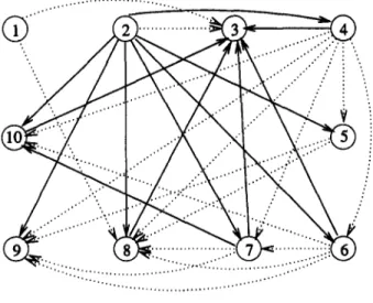
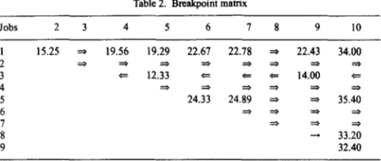
By the example given in Table 1, we try to figure out the effect of last dominance rule on the number of global dominances generated and the corresponding lower bound values. In Fig. 7, the dashed lines represent the global dominances found by Rinnooy Kan et al. generalizations and the bold lines represent the additional global dominances added by the proposed dominance rule. The number of edges generated by the first three conditions is 17 and the lower bound value is 1. When the additional global dominance rule is considered, the number of edges increases by 13, which makes the total of 30. Consequently, the lower bound value increases to 40. Furthermore, the proposed dominance rule provides the breakpoint values as a function of time as shown in Table 2. In the matrix of breakpoints, the following notation is used: the numbers in cells correspond to the breakpoints, the global precedences ( ~ ) and unconditional precedences (---.). A more detailed discussion on the computational results can be found in Section 6.
5.2. Linear lower bound
The linear lower bound is originally obtained by Ports and Van Wassenhove [8] by using the Lagrangian Relaxation approach with subproblems that are total weighted completion time problems.
. , ' . . . ' " . t
--..:::::::: ... !!}!ii;Jl..S.i.:i'il ... ... ....
... E m m o n s ' Dominance
Table 2. Breakpoint matrix Jobs 2 3 4 5 6 7 8 9 10 1 15.25 ~ 19.56 19.29 22.67 22.78 ~ 22.43 34.00 3 ~ 12.33 = = = 14.00 4 :::* ::o =0 =0 ==* :=~ 5 24.33 24.89 ~ ~ 35.40 6 ~ ~ ~ 7 ~ ~ 20 8 ~ 33. 9 32.40
Abdul-Razaq et al. [1] show that it may also be derived by reducing the total weighted tardiness criterion to a linear function, i.e. total weighted completion time problem. For the job i(i= 1 ... n), we have
wiTi =wi max{ Ci - dl,0)---u~ max{ Ci - di,0} >-ui(Ci - eli),
where w~>-u~>-O and C~ is the completion time of job i. Let u = ( u l ... un) be a vector of linear weights, i.e. weights for the linear function C,.-d~, chosen so that O<-ui<-wi. Then a lower bound is given by the following linear function
LBLin(u)= ~ i=1 ui(C i - d i ) < - ~ w i i=1 max{ (2,. - d/,0}.
This shows that the solution of total weighted completion time problem provides a lower bound on the total weighted tardiness problem. Given u, the total weighted completion problem can be solved optimally by the WSPT rule in which the jobs are sequenced in non increasing order of u/p~. To obtain the linear lower bound, an initial sequence is required to determine job completion times C~. Then the vector of linear weights u is chosen to maximize LBLin(U), subject to u~<-w~ for each job i. Abdul-Razaq et al. [1] compare several lower bounding approaches and their computational results indicate that the linear lower bound is superior to others in the literature due to its quick computability and low memory requirements. We will test the impact of an initial sequence on the linear lower bound value and try to demonstrate having a better, i.e. near the optimal, upper bound value will improve the lower bound value. In Section 6, we will show how the proposed dominance rule can be used to improve the weighted tardiness criterion to obtain a better initial sequence.
6 . C O M P U T A T I O N A L R E S U L T S
We tested each lower bounding scheme on a set of randomly generated problems on a Sun Ultra Spare 1 workstation using Sun Pascal. The lower bounding scheme was tested on problems with 50, 100 and 150 jobs that were generated as follows. For each job i, an integer processing time Pi and an integer weight wi were generated from two uniform distributions, [1,10] and [1,100] to create low or high variation, respectively. The relative range of due dates, RDD and average tardiness factor, TF were selected from the set {0.1, 0.3, 0.5, 0.7, 0.9}. An integer due date d; from the uniform distribution [P(1 - T F - RDD/2), P(1 -TF+RDD/2)] was generated for each job i, where P is the total processing time, E i~ ~i. As summarized in Table 3, a total of 300 example sets were considered and 100 replications were taken for each combination resulting in 30,000 randomly generated runs.
First, we have tested LB~ which uses the global dominance information for calculating the lower bound. We have calculated the average lower bound values (LB-Value), average improvement (lmprov), average number of global dominances generated (Glob.) and the average real time used in centiseconds (Time). Although the real time depended on the utilization of system when the measurements were taken, it was a good indicator for the computational requirements, since the CPU times were so small that we could not measure them accurately. In general, the actual CPU time is considerably smaller than the real
Table 3. Experimental design
Factors No. of levels Settings
Number o f jobs 3 100, 300, 500
Processing time variability 2 [1, 10], [1, 100]
Weight variability 2 [1, 10], [1, 100]
Relative range o f due dates 5 0.1, 0.3, 0.5, 0.7, 0.9
Table 4. The effect of the new dominance rule
n=50 n=100 n=150
Criteria > = < > = < > = <
LB value 5340 4660 0 5824 4176 0 6160 3840 0
No. of ares 7362 2638 0 7344 2656 0 7297 2703 0
time. The improvement in the lower bound for each run is found as follows: Improv= [(F(S D) -F(sh))/ F(Sh)] × 100, if F(sh)#0, and zero otherwise, where F(S h) is the lower bound value obtained by the Rinnooy Kan et al. generalizations and F(S °) is the lower bound value given by the proposed dominance rule. We also performed a paired t-test for the difference between lower bound values generated by these rules for each run.
In Tables 4--6, we give the statistics about the effect of Emmons' rules (EDR), including the Riunooy
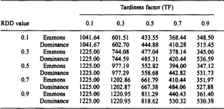
Kan et aL generalizations, and the proposed dominance rule (PDR). (>) represents the number of cases in which PDR gives better results than EDR, where as (=) represents number of cases in which PDR gives results as well as EDR and (<) represents cases for which EDR gives better results. Both the lower bound value and number of arcs (global dominances) generated by PDR dominate EDR as indicated in Table 4. In Table 5, the results are averaged over 10,000 runs for 50, 100 and 150 job cases. The large t-test values and the average percentage improvement indicate that there is a significant improvement in the lower bound value. In Table 6, we present the effect of RDD and TF on the number of global dominances generated by PDR and EDR for 50 job case. For TF = 0.1, almost all of the relations can be defined by global dominances, so both Emmons' and the proposed dominance rule can solve the problem optimally. While for TF-0.3, the number of global dominances decreases substantially, but still PDR dominates EDR.
In order to find an initial sequence for the linear lower bound, we have selected a number of heuristics and their priority indexes are summarized in Table 7. The EDD, WSPT, SPT and LPT are examples of static dispatching rules, where as ATC and COVERT are dynamic ones. Vepsalainen and Morton [14] have shown that the ATC rule is superior to other sequencing heuristics and close to the optimal for the lllY.wiTt problem. Furthermore, we have already shown that if any sequence violates the dominance rule, then the proposed algorithm discussed in Section 4 either lowers the weighted tardiness or leaves it unchanged. First, we use one of the dispatching rules to find an initial sequence, later we apply the algorithm to get the sequence denoted as Heuristic+DR. For each heuristic, we have calculated the average lower bound value before and after implementing the algorithm along with the average improvement, (improv), as summarized in Table 8. ATC, COVERT, and WSPT seem to perform better
Table 5. Comparison of Emmons' rule with the proposed rule
n LB-Value Improv (%) Time Glob. t-test
Emmons Domin. Emmons Domin. Emmons Domin.
50 23591.9 36988.9 85.1 4.06 5.98 694.8 743.7 31.53
100 88391.1 140194,6 96.19 18.7 27.5 2827.5 3021.3 32.09
150 189130.8 296505.1 102.7 49.8 73.1 6411.2 6830.7 31.84
Table 6. Number of global dominances for n=50 Tardiness factor (TF) 0.I Emmons 1041.64 601.51 433.55 368.44 348.50 Dominance 1041.67 602.70 444,88 410.28 515.45 0.3 Emmons 1225.00 744.08 477.04 378.14 345.06 Dominance 1225.00 744.59 485.31 420.44 536.59 0.5 Emmons 1225.00 977.19 552.82 394.00 347.12 Dominance 1225.00 977.29 558.68 442.82 531.73 0.7 Emmons 1225.00 1202.86 661.79 410.44 351.97 Dominance 1225.00 1202.87 667.38 484.06 527.88 0.9 Emmons 1225.00 1220.95 811.29 440.43 361.40 Dominance 1225.00 1220.95 818.62 530,32 530.38 RDD value 0.1 0.3 0.5 0.7 0.9
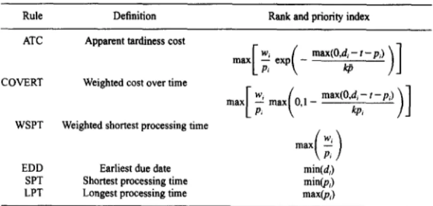
Table 7. Dispatching rules used in lower bounding scheme
Rule Definition Rank and priority index
ATC Apparent tardiness cost
max[~exp(-max(O'd~ut-P))]
COVERT Weighted cost over time
ma×[ ~ max(O,1
max(O'd~-t-P')~l
WSPT Weighted shortest processing time
EDD Earliest due date min(dt)
SPT Shor~st processing time min(pt)
LPT Longest processing time max(p~)
than other heuristics when the dominance rule is applied to get the local optimal sequence. We have tested each heuristic over 10,000 runs for 50, 100 and 150 job cases in Table 9. As discussed above, (>) represents number of runs in which the sequence obtained from Heuristic+DR gives a higher linear lower bound value than the sequence obtained from the heuristic, where as (=) represents number of runs in which Heuristic+DR performs as well as heuristic, and (<) represents number of runs in which Heuristic +DR performs worse. For example, the EDD +DR combination performed 4598 times better (>) than the EDD rule. The large t-test values on the average improvement indicate that the proposed dominance rule provides a significant improvement on all rules and the amount of improvement is notable at 99.5% confidence level for all heuristics.
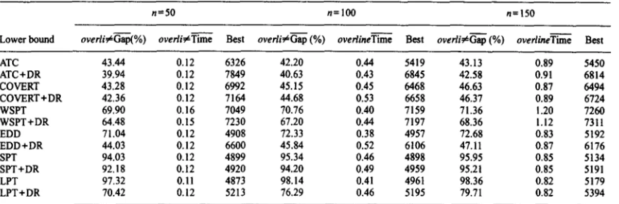
In Table 10, we summarize the average percent gap, real time consumed in centiseconds and number of times the lower bound value of a heuristic outperforms others over 10000 runs. Notice that more than one heuristic can have the "best" value for a certain run if there is a tie. The average gap botween heuristic and its lower bound, (gap) for each run is found as follows: gap=[(F(S L~) -F(SLa))/F(St~)] x 100, if F(SUa)~0, and zero otherwise, where
F(S t~)
is the total weighted tardiness value obtained by the heuristic and F(S LB) is the corresponding lower bound value. It can be seen that Heuristic+DR always performs better than the heuristic alone. Furthermore, the average real time consumed for each dispatching rule is very small, i.e. the maximum time used is 1.2 centiseconds for n = 150. The average time consumed by LBj is higher than other methods. The time for LB1 includes both the calculations for the breakpoint matrix and testing the dominance rules while the linear lower bound assumes that an initial sequence is given. In summary, we can reach to the following conclusions from these results. The lower bound value of LB1 is not as good as the linear lower bound method, but it can be used in B&B algorithms because it contains the global dominance information which will restrict the search spaceTable 8. Linear lower bound: computational results for
n=50
Upper bound Lower bound
Heuristic Before After hnprov (%) Before After Improv (%)
ATC 119721.1 118569.8 6.26 103248.1 103295.6 0.10 COVERT 127375.3 125861.9 3.96 97996.1 98215.6 0.58 WSPT 153656.5 134254.7 49.41 100286.7 103020.8 1.09 EDD 275662.4 128032.7 39.55 26174.3 93948.9 103.65 SPT 228100.5 213260.4 18.10 18803.5 21049.4 7.45 LPT 535667.8 152872.4 81.05 19031.5 76026.4 147.64
Table 9. Comparisun of linear lower bounds
n=50
[n= 100] n=150Heuristic > = < t-test > r. < t-test > = < t-test
ATC+DR 2490 7499 11 23.16 2531 7405 64 24.10 2555 7315 130 24.35 COVERT+DR 447 9406 147 3.56 661 9044 295 4.24 858 8834 308 4.21 WSPT+DR 2462 7532 6 22.58 2426 7566 8 22.44 2405 7584 11 21.95 EDD+DR 4598 5176 226 31.73 4463 5202 335 31.16 4368 5346 286 30.55 SPT+DR 3516 6221 263 24.26 3904 5857 259 23.76 3995 5763 242 29.53 LPT+DR 4772 5008 220 32.68 4742 5005 253 31.87 4582 5221 197 31.39
Table 10. Overall computational results
n=50 n= lO0 n=lS0
_ _ B _ _
Lower bound overli#Gap(%) overli#Time Best overli#Gap (%) overlineTime Best overli~Gap (%) overlineTime Best
ATC 43.44 0.12 6326 42.20 0.44 5419 43.13 0.89 5450 ATC+DR 39.94 0.12 7849 40.63 0.43 6845 42.58 0.91 6814 COVERT 43.28 0.12 6992 45.15 0.45 6468 46.63 0.87 6494 COVERT+DR 42.36 0.12 7164 44.68 0.53 6658 46.37 0.89 6724 WSPT 69.90 0.16 7049 70.76 0.40 7159 71.36 1.20 7260 WSPT+DR 64.48 0.15 7230 67.20 0.44 7197 68.36 1.12 7311 EDD 71.04 0.12 4908 72.33 0.38 4957 72.68 0.83 5192 EDD+DR 44.03 0.12 6600 45.84 0.52 6106 47.11 0.87 6176 SPT 94.03 0.12 4899 95.34 0.46 4898 95.95 0.85 5134 SPT+DR 92.18 0.12 4920 94.20 0.49 4959 95.21 0.85 5191 LPT 97.32 0.ll 4873 98.14 0.41 4961 98.36 0.82 5179 LPT+DR 70.42 0.12 5213 76.29 0,46 5195 79.71 0.82 5394
quite substantially. The linear lower bound gives the tightest lower bound value and either the ATC + DR or WSPT+DR can be used as an initial sequence.
7. C O N C L U S I O N
In this paper, we prove that there are certain time points, called as breakpoints, in which the ordering changes for adjacent jobs, such that the arrangement of these jobs in an optimal schedule depends on their start times. Based on these results, we have developed a new dominance rule for the lllEwf,, problem which provides a sufficient condition for local optimality. Therefore, a sequence generated by the proposed rule cannot be improved by adjacent job interchanges. We also enlarge the region for which the lllEwf,- problem can be solved optimally by the WSPT rule. The proposed dominance rule covers and extends the Emmons' results, including Rinnooy Kan et al. generalizations, by considering the time dependent ordefings between each pair of jobs, so that tighter upper and lower bounds are found as a function of start time of this pair. Furthermore, it can be used as a good pruning device for any exact algorithm. We have implemented the proposed rule in two different lower bounding schemes. Our computational experiments over 30,000 randomly generated problems indicate that the amount of improvement is statistically si~ificant for both methods. For further research, we will look at how the proposed dominance properties can be incorporated in a B&B solution methodology in conjunction with a branching strategy.
Acknowledgements--The authors would like to thank an anonymous referee for pointirtg out a more elegant and intuitive proof to the derivations o f breakpoints than we had originally included.
R E F E R E N C E S
I. Abdul-Razaq, T. S., Ports, C. N. and Van Wassenhove, L. N., A survey o f algorithms for the single-machine total weighted tardiness scheduling problem. Discrete Applied Mathematics, 1990, 26, 235-253.
2. Chambers, R. J., Carraway, R. L., Lowe, T. J. and Morin, T. L., Dominance and decomposition heuristics for single machine scheduling. Operations Research, 1991, 39, 639---647.
3. Emmons, H., One machine sequencing to minimize certain functions of job tardiness. Operations Research, 1969, 17, 701-715.
4. Fisher, M. L., A dual algorithm for the one-machine scheduling problem. Mathematical Programming, 1976, 11,229-251. 5. Hoogeveen, J. A. and Van de Velde, S. L., Stronger Lagrangian bounds by use of slack variables: Applications to machine
scheduling problems. Mathematical Programming, 1995, 70, 173-190.
6. Jensen, J. B., Philipoom, P. R. and Malbotra, M. K., Evaluation o f scheduling rules with commensurate customer priorities in job shops. Journal of Operations Management, 1995, 13, 213-228.
7. Lawler, E. L., A "pscudopolynomial" algorithm for sequencing jobs to minimize total tardiness. Annals of Discrete Mathematics, 1977, 1, 331-342.
8. Potts, C. N. and Van Wasscnhove, L. N., A branch and bound algorithm for total weighted tardiness problem. Operations Research, 1985, 33, 363-377.
9. Ports, C. N. and Van Wassenhove, L. N., Dynamic programming and decomposition approaches for the single machine total tardiness problem. European Journal of Operational Research, 1987, 32, 405-414.
10. Rachamadugu, R. M. V., A note on weighted tardiness problem. Operations Research, 1987, 35, 450-452.
11. Rinnooy Karl, A. H. G., Lageweg, B. J. and Lanstra, J. K., Minimizing total costs in one-machine scheduling. Operations Research, 1975, 23, 908-927.
12. Szwarc, W., Adjacent orderings in single machine scheduling with earliness and tardiness penalties. Naval Research Logistics,
1993, 40, 229-243.
13. Szwaro, W. and Liu, J. J., Weighted tardiness single machine scheduling with proportional weights. Management Science,
1993, 39, 626-632.
14. Vopsalainon, A. P. J. and Morton, I". E., Priority rules for job shops with weighted tardiness costs. Management Science, 1987, 33, 1035-1047.