Global many- to - many aligment of multiple protein-protein interaction networks

(1)

GLOBAL MANY-TO-MANY ALIGNMENT OF MULTIPLE PROTEIN-PROTEIN INTERACTION NETWORKS

FERHAT ALKAN

(2)

F er h at A lk an M .S . T h es is 2 0 1 3

(3)

INTERACTION NETWORKS

by Ferhat Alkan

Bachelor’s degree, Telecommunication Engineering, Istanbul Technical University, 2010

Submitted to the Graduate School of

Science and Engineering in partial fulfillment of the requirements for the degree of Computer Engineering

Master of Science

Kadir Has University 2013

(4)

GLOBAL MANY-TO-MANY ALIGNMENT OF MULTIPLE PROTEIN-PROTEIN INTERACTION NETWORKS

APPROVED BY:

Assoc. Prof. Dr. Cesim Erten . . . . (Thesis Supervisor)

Asst. Prof. Dr. ¨Oznur Ya¸sar Diner . . . .

Asst. Prof. Dr. Tınaz Ekim A¸sıcı . . . .

(5)

ABSTRACT

GLOBAL MANY-TO-MANY ALIGNMENT OF MULTIPLE

PROTEIN-PROTEIN INTERACTION NETWORKS

Proteins are the essential parts of organisms and almost every biological process within a living cell is mediated by proteins and their interactions. Due to such importance, proteins are at the core of many researches in systems biology and evolutionary biology. In particu-lar, defining the function of a protein and identifying functionally orthologous proteins are crucially important in many research areas and precise function of a protein can only be de-fined by biochemical and structural studies. However, many computational methods are also developed for such purposes and they use the sequence and interaction data of proteins since it provides a presumption about the chemical structure of a protein. For example, network alignment studies aims to find clusters of functionally related proteins across given protein interaction networks usually by implementing the given networks as graphs and employing some graph theoretical approaches. In this thesis, we focus on the problem of global many-to-many alignment of multiple protein-protein interaction networks. We define the problem as an optimization problem and this is the first combinatorial definition that is given for the problem in the literature. Then, we prove the computational intractability of this problem and we propose a new heuristic algorithm for the solution. We provide the test results of the proposed algorithm on both actual and synthetic PPI networks and it outperforms the existing algorithms, that serve at similar purpose, in terms of many evaluation aspects.

(6)

¨

OZET

B˙IRDEN C

¸ OK PROTE˙IN ETK˙ILES

¸ ˙IM A ˘

GININ C

¸ OKA C

¸ OK

OLARAK H˙IZALANMASI

Proteinler canlı organizmaların temel yapıta¸slarını olu¸sturur ve hücreler i¸cerisindeki bir¸cok biyolojik süreci düzenlerler. Bu büyük önemleri nedeniyle de sistem biyolojisi ve evrimsel biyoloji alanlarında bir¸cok ara¸stırmanın oda˘gı halindedirler. Ozellikle protein-¨ lerin fonksiyonlarının tanımlanması ve fonksiyonel olarak benzer proteinlerin gruplanması bir¸cok ara¸stırma alanı i¸cin büyük önem ta¸sımaktadır. Fakat bir proteinin kesin fonksiy-onu ancak biyokimyasal ve yapısal analizlerle bulunabilmektedir. Bununla beraber protein-lerin dizilim ve etkile¸sim bilgiprotein-lerini kullanarak bu ama¸clara hizmet eden hesapsal yöntemler de geli¸stirilmektedir. Örne˘gin a˘g hizalama ¸calı¸smaları bunlardan biridir ve verilen protein a˘gları i¸cerisinden fonksiyonel olarak birbirine benzeyen proteinleri kümelemeyi ama¸clar. Bu ¸calı¸smalar genellikle verilen a˘gların ¸cizgeler olarak tanımlanmasını ve bu ¸cizgeler üzerinde ¸ce¸sitli ¸cizge teorik yakla¸sımlar uygulanmasını i¸cerirler. Bu tez kapsamında ise birden ¸cok protein a˘gının ¸coka ¸cok olarak hizalanması problemi ele alınmaktadır. Bu tez ile bu hiza-lama problemi bir optimizasyon problemi olarak tanımlanmakta ve bu tanım bu problem i¸cin literatürde verilmi¸s olan ilk kombinatöryel tanımdır. Daha sonra bu problemin i¸slemsel karma¸sıklı˘gı analiz edilmekte ve problemin ¸cözümü i¸cin bir bulu¸ssal algoritma önerilmektedir. Sunulmu¸s olan BEAMS algoritmasının hem ger¸cek hemde sentetik a˘glar üzerindeki test sonu¸cları sunulmakta ve bu sonu¸clar literatürde aynı amaca hizmet eden di˘ger algoritmalar ile kar¸sıla¸stırıldı˘gında, BEAMS algoritmasının bir¸cok a¸cıdan di˘ger benzer algoritmalardan daha etkili ¸calı¸stı˘gı görülmektedir.

(7)

ACKNOWLEDGEMENTS

I would like to thank many people who helped to make my graduate school days most valuable and productive but first, I sincerely thank Assoc. Prof. Cesim ERTEN, my major professor and thesis advisor. It was not only intellectually rewarding but also convivially pleasant to work with him in these two years. I also thank him for introducing me to the very interesting field of Bioinformatics.

Many thanks to faculty research assistants, who sincerely gave me a warm welcome when I first enrolled to this graduate programme. Particularly, special thanks to Aykut C¸ ayır for his valuable friendship and Serkan Altunta¸s for his informative comments about biological background of this thesis. I would also like to thank to all professors of computer engineering department for their highly instructive courses.

The last words of thanks go to my family and my beloved friends. I thank my parents Mete & Fatma Alkan and my brother Köksal Alkan for their endless support and encourage-ment. Lastly I thank my dearest friends Aysima Kar¸caaltıncaba, Do˘gu¸s Burak Akkoyunlu, Ekin Önsöz, Emre Sofyalı, Ezgi Toksoy, Taner Öz and all my other friends for their presence in my life.

(8)

This work is dedicated to the brave chapullers who are killed and injured during the Taksim Resistance in June 2013,

(9)

LIST OF FIGURES

Figure 1.1. Visual description of network alignment problem (taken from [1]). . . . 6

Figure 2.1. Conservation scores on a sample alignment covering all notable cases. . 12

Figure 2.2. Sample neighborhood graph construction and candidate generation for a small instance. . . 15

Figure 3.1. Construction of the clause gadget for a clause ci = (xp∨ xq∨ xr) and the

variable gadgets for xp, xq, xr of Proposition 3.1.1. . . 21

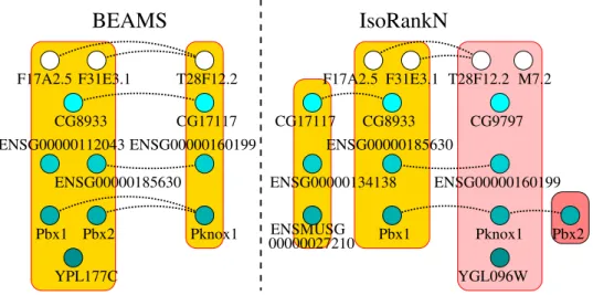
Figure 5.1. Comparative visualization of a sample clustering produced by the BEAMS and the IsoRankN algorithms running on the IsoBase data. Both clusters of the BEAMS alignment are consistent. Only the two leftmost clusters of the IsoRankN alignment are consistent. . . 40

(12)

LIST OF TABLES

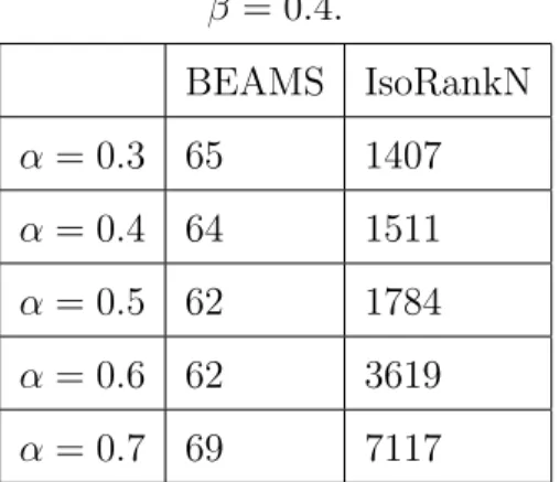
Table 4.1. Required CPU times in minutes for both algorithms executing on the IsoBase data for five networks. The BEAMS algorithm is executed with

the parameter setting of β = 0.4. . . 33

Table 5.1. Analysis of Output Clusters . . . 36

Table 5.2. Biological Significance Evaluations. . . 38

Table 5.3. Analysis of Output Clusters for CG Network Family. . . 44

Table 5.4. Analysis of Output Clusters for DMC Network Family. . . 45

Table 5.5. Analysis of Output Clusters for DMR Network Family. . . 46

Table 5.6. Functional Consistency Evaluation for the Alignment of CG Network Family. . . 47

Table 5.7. Functional Consistency Evaluation for the Alignment of DMC Network Family. . . 48

Table 5.8. Functional Consistency Evaluation for the Alignment of DMR Network Family. . . 49

(13)

1. INTRODUCTION

This introductory chapter is divided into four sections to provide better understanding of the biological background of the thesis. We first start by giving information about genes, gene products, their functions and sequence alignment. Then, we give information about the functional orthology of genes and proteins and we continue by explaining protein interaction networks. In the last section, network alignment is introduced to the reader and existing alignment algorithms are summarized for a better understanding of global network alignment problem.

1.1. Genes, Proteins and Comparative Genomics

Every living organism is made of cell or cells and all living organisms carry out count-less different biological activities during their lifetime. Most of these biological activities take place inside the cells and these cellular processes are always mediated by some specific molecules and their interactions with other molecules. In particular, proteins and their inter-actions are at the core of many cellular processes and these proteins are mostly synthesized within the cells of organisms.

The information to synthesize such proteins is mostly inherited from the ancestors of the cell and it is part of the genetic information that is handed down from generation to generation through their genomes. DNA molecules in genomes store this information in a chemical code with its chemical building blocks and the interpretation machinery of this code is essentially the same for every species [2]. According to the central dogma of biology, chemical code of the needed information is first transcribed into a chemically related set of molecules, messenger RNA (mRNA) and then, this coded information in mRNA is translated into a chemically related protein molecule in ribosome, a special organelle of the cell. The

(14)

information-carrying transcribed parts of the DNA molecules are called as genes and thereby proteins are considered as the products of their coding genes.

Amino-acids are the fundamental building blocks of proteins and every protein has an amino-acid sequence which is determined by the chemical code sequence of its coding gene. The amino-acid sequence and the folding of protein determines its specific three dimensional structure and this structure lies at the core of determining its interactions and function within the cell.

Breakthrough advances in sequencing technology of genomes and proteins resulted in huge amount of fruitful sequence data of genomes and proteins for many species. Due to this progress, a new field of study, comparative genomics was born and it aims to provide insights about the evolutionary and functional mechanisms on genomes by comparing sequence data of different genes and gene products that are from different species. As mentioned by Fang et al., all species originates from a common ancestor and these variations are because of the natural selection and being exposed to different complicated environmental changes. They continue by stating, with the field of comparative genomics, divergence of species from the common ancestor can be deciphered by comparing genomes of different organisms and, evolutionary processes such as gene deletion, gene speciation, gene duplication and horizontal gene transfer cause additional complexity for current comparisons [3]. Therefore, these complexities have forced researchers to develop different aspects for analyzing the data which is highly increasing in quantity and quality. So far, there have been many breakthrough progresses and many tools have been created for such comparisons. For example, ”Basic Local Alignment Search Tool (BLAST)” [4] is one of the most important tools that is used for measuring how similar two genes and two gene products are in their sequences.

(15)

1.2. Functional Orthology of Genes and Proteins

Evolutionary processes on genomes cause speciation, duplication and deletion of genes and that is the reason why species have different DNA sequences in their genomes despite the origination from a common ancestor. If two genes share a common ancestral gene, they are called as homologs and there are two types of homologous genes. If these genes belong to the different species they are called as orthologs and otherwise called as paralogs [5]. In other words, if two genes in different species have evolved through speciation processes they become orthologous and if two genes from the same specie have evolved through duplication processes they become paralogous [5]. Whether they are paralogous or orthologous, homologous genes are mostly similar to each other in their sequences.

In comparative genomics, accurate orthologous gene identification bears a crucial im-portance for many other research areas such as gene function prediction, phylogenetic anal-yses, and genomic context analyses [5] and there is a large variety of proposed orthologs prediction methods in literature [6, 7, 8, 9, 10, 11, 12, 13]. Orthologous genes and proteins are also analyzed to identify whether they share the same function in their cellular pro-cesses. Generally it is assumed that orthologous proteins are functionally related but they need further analyses to identify their functional orthology.

Defining a function for proteins is still an extensively studied area of proteomics science and sequence alignment tools and interaction data of proteins are intensively used in this area. Accurate function prediction for a protein can only be achieved by biochemical and structural studies, however, due to the high quantity of proteins, it is impossible to perform such studies for every protein in all species. For this reason, development of reliable computational methods for protein function prediction bears a crucial importance to progress in genomics science. So far developed computational methods for such predictions mostly rely on the sequence alignment and interaction data of proteins and they are proven to be reliable in

(16)

many ways. Besides, representing the interaction data of proteins as networks comes in handy for such function prediction studies.

1.3. Protein-Protein Interaction (PPI) Networks

As mentioned before, cellular activities of all organisms are mostly mediated by pro-teins and their interactions. Technological advances, several high throughput measurement techniques and computational methods enabled to discover these protein-protein interac-tions (PPIs) for many species and these interacinterac-tions are at the center of many researches in many areas. According to Singh et al. [14], ”the data from these techniques, which are still being perfected, are being supplemented by high-confidence computational predictions and analyzes of PPIs [15, 16, 17]”. For better analysis and representation, many complex sys-tems in biology such as PPIs, metabolic processes, gene regulations and signal transductions are usually represented by networks and structural information of PPI networks for many species are becoming increasingly complete and accurate with those techniques. With the availability of these networks, new area for systematic studies of PPI networks was born and especially, cross-species network comparisons have taken a considerable interest from many researchers. In many computational comparison studies, these networks are implemented with graphs where nodes represent the proteins and the edges correspond to interactions between pairs of proteins.

Network comparison can provide valuable insights about the structural and organi-zational features of PPI networks [18] and by discovering network similarities of different species, valuable insights can be developed about the evolution, cellular biology and maybe diseases. For these reasons, as mentioned by Sharan and Ideker, three types of network com-parison methods has been suggested in general and these methods are network integration, network querying and network alignment [1].

(17)

Network integration is the study of comparing PPI network of a specie with other net-works of the same specie. This other compared network can be metabolic, signal transduc-tion or gene regulatory network and by this method it is aimed to discover the interrelatransduc-tions within the specie which can also result in function prediction for the proteins in the PPI net-work [19]. Furthermore, netnet-work querying studies aim to find subnetnet-works in a PPI netnet-work that is similar to the desired subnetwork whether from the same specie or different species and by this querying, it is aimed to develop knowledge about the evolutionary processes as it is mentioned in such articles [20, 21, 22, 23, 24, 25, 26]. Network alignment, which is also the main topic of our interest in this thesis, is explained in more detail in the next section.

1.4. Network Alignment of PPI Networks

Network alignment is the study of comparing two or more networks to identify similar or dissimilar regions across given networks. Network alignment of PPI networks is a crucially important study area in comparative genomics since it provides a better understanding and gives valuable insights in many areas, such as functional module conversation across species, functional orthologous proteins identification, prediction of homologous proteins and creation of phylogenetic relationships between different organisms. For such different purposes, two different network alignment type exists which are local network alignment and global network alignment. Additionally, if alignment is performed only with two networks it is named as pairwise alignment but if performed with more networks, it is named as multiple alignment. Figure 1.1 illustrates the network alignment problem.

As mentioned by Singh et al., whether it is local or global, network alignment algo-rithms generally aim to reveal one or more common subgraphs across the graphs of given input networks and the uniformity of these graphs make way for conserving edges of these subgraphs. They continue by stating that, this conservation leads to a mapping between the nodes (proteins) from different networks but the difficulty is to create such mappings

(18)

Figure 1.1. Visual description of network alignment problem (taken from [1]).

which are evolutionarily related [14]. Therefore, network alignment algorithms do not only deal with the network topologies of input networks to decide alignments, they also consider evolutionary relations of proteins such as their sequences since sequence similarities could represent evolutionary relations.

Additionally, alignment algorithms may also differ with respect to the types of map-pings they provide. One-to-one alignment approaches aim to generate alignments where the output alignment either maps a protein in a network to exactly one protein from one of the networks or leaves the protein unmapped [14, 27, 28]. One-to-many alignments have been proposed for the global alignment of other biological networks including metabolic pathways, where each metabolic reaction in a pathway is mapped to a subset of reactions from another pathway [29, 30]. Finally, for many-to-many alignments the goal is to extract clusters of proteins where each cluster may include any number of proteins from the input networks [31, 32]. The proteins mapped to the same cluster as a result of the alignment are all expected to compose a functionally orthologous group. Note that among all three

(19)

versions of the network alignments, the many-to-many version is the most general. Further-more, as far as constraints from evolutionary molecular biology are concerned, it provides a more intuitive definition; the evolutionary distance between organisms under study may have large variations, leading to different numbers of proteins functioning similarly when considered in different networks.

In the following subsections, we continue by giving more detail about local and global network alignments.

1.4.1. Local Network Alignment

Local network alignment aims to discover highly similar structured subgraphs in given network graphs and it is performed for detecting similar functional modules in different species. At the early stages of network alignment algorithms, instead of global alignment al-gorithms, many local alignment algorithms have been developed and proposed. For example, NetworkBLAST [33] and PathBLAST [21] adapted the underlying ideas of BLAST sequence alignment algorithm; Graemlin [34] used protein modules for producing alignments; Berg and Lassig [35] has used Bayesian approach; MaWish [36] used evolution based scoring and Narayanan and Karp [37] performed a graph matching algorithm. However, Singh et al. states that, all these algorithms mostly rely on sequence similarities of proteins to reduce the complexity of problem so that they suffer from not considering network topologies in a significant level [14].

The outcomes of local network alignment algorithms provide clues about the functions of proteins by having many proteins of the same known function in the same detected common subgraph and in such situations, it is expected that remaining functionally unknown proteins of that subgraph have the same function as the rest.

(20)

1.4.2. Global Network Alignment

Informally, global alignment of multiple PPI networks is the problem of generating functional orthologous disjoint protein clusters through given networks. Since functional orthology is both about the interactions and sequences of proteins, global alignment seeks to create any kind of mapping between all proteins of given networks that will conserve the network topology and ensure the mapped proteins are highly sequence similar to each other. Zaslavskiy et al. states that, it is a more challenging problem than local alignment from a computational point of view since it searches for the best global mapping solution among all global possibilities [38]. They continue by stating, global alignment problem can also be considered as the problem of finding weighted graph matching between given PPI network graphs [38].

For all global network alignment algorithms, integration of network topology and se-quence similarities has a crucial role. Alada˘g and Erten states that, ”Network alignment algorithms on the other hand incorporate the interaction data as well as the evolutionary re-lationships represented possibly in the form of sequence data. Based on the assumption that the interactions among functionally orthologous proteins should be conserved across species, such incorporation is usually achieved by aligning proteins so that both the sequence simi-larities of aligned proteins and the number of conserved interactions are large” [38].

Lately, global alignment problem has taken considerable interest and many algorithms are proposed for the problem solution. Some of them are GA [38], NATALIE [39], Ne-tAlignBP, NetAlignMR [40], Graemlin [34], IsoRank [14], IsoRankN [32], MI-GRAAL [41] and variants [42], algorithm of Shih and Parthsarathy [37] and SPINAL [28]. Among all these existing algorithms, only IsoRankN algorithm is introduced in this thesis since it is the latest and so far best algorithm about global many-to-many alignment of multiple protein interaction networks.

(21)

IsoRankN algorithm generates the many to many clusters of global alignment results in two phases. In the first phase, it calculates a functional similarity score for each cross-species protein pairs, where it balances the the topological similarity and sequence similarity of the proteins with a user defined value α. Functional similarity score generation is performed by the original IsoRank algorithm and it uses a spectral graph theory for these calculations. Then, IsoRankN constructs a similarity graph with these scores and it performs a star aligned approach on this graph. After the creation of stars which is based on generated similarity scores, it performs spectral partitioning method on generated stars to decide final clusters.

1.5. The Scope and Contribution of the Thesis

The focus of this thesis is on global many-to-many alignment of multiple PPI networks. We first provide a formal combinatorial definition of the problem and it is the first formal definition in the literature. We proceed with proving its computational intractability even in a quite restricted case. We next provide a general framework for the problem, where we decompose the original problem into two subproblems; that of backbone extraction and backbone merging. Informally, each backbone in this framework corresponds to a closely related central group of proteins, at most one from each network. Once all the backbones are determined, the latter subproblem involves merging together the backbones with higher chances of coexistence in a cluster of orthologous proteins. We provide heuristic methods for both subproblems which together form our proposed algorithm based on backbone extraction and merge strategy, BEAMS. We experimentally evaluate the algorithm with regards to several biological significance metrics proposed in literature and compare it against a state-of-the-art and one of the most popular global many-to-many alignment methods, IsoRankN. The experimental results indicate that BEAMS alignments provide more consistent clusters than those of IsoRankN. Furthermore, considering the heavy computational load of the problem, the exceptional running time of BEAMS as compared to that of IsoRankN is a further improvement resulting from the provided framework and the algorithm.

(22)

2. METHODS AND ALGORITHMS

In this chapter, we first define the problem of global many-to-many alignment of mul-tiple PPI networks as an optimization problem. Later on, we propose a new heuristic algo-rithm for the solution. Proposed algoalgo-rithm is named as BEAMS after its method Backbone Extraction And Merging Strategy which will be explained in following sections.

2.1. Problem Definition

Although the one-to-one version of the problem has been formally defined in previous work [28], no formal combinatorial definition exists for the many-to-many version of the alignment problem apart from parameter learning based definitions [34]. We first provide a formally defined optimization goal for the problem that captures the essence of the informal definition provided in the Introduction. The definition is based on an intuitive generalization of the global one-to-one network alignment problem definition provided in [14, 28].

Let G1(V1, E1), G2(V2, E2), . . . , Gk(Vk, Ek) be the input PPI networks where Gi

cor-responds to the ith _{PPI network and} _V

i, Ei denote respectively the vertex set (proteins)

and the edge set (interactions) of Gi. Let S indicate the edge-weighted complete k−partite

similarity graph where the ith _{partition of} _{S is V}

i and each edge (u, v) in S is assigned a

positive real weightw(u, v). This weight corresponds to the sequence similarity score s(u, v) betweenu and v, usually assumed to be the Blast bit score of u and v, where u ∈ Gi,v ∈ Gj

and i 6= j. Let Sβ be a subgraph of S with the same set of vertices. Sβ represents a filtered

version of the similarity graphS, so that only edges between pairs of proteins with relatively high sequence similarity are retained. For a fixed Sβ, the global many-to-many alignment

(23)

clusters CL = {Cl1, Cl2, . . . , Clm} that maximizes the following alignment score:

AS(CL) = α × CIQ(CL) + (1 − α) × P

∀Cli∈CLICQ(Cli)

|CL| (2.1)

Hereα is a real number between 0 and 1. It is a balancing parameter that determines the contribution weight of network topology as compared to homological similarity in the construction of output alignments. Each cluster Cli is defined to be a complete c−partite

subgraph ofSβ where 1< c ≤ k. A set of clusters CL is maximal if no additional clusters can

be added to CL, that is no further complete c−partite subgraph remains in Sβ. Note that

maximizing theAS score does not automatically guarantee the maximality of the output set of clusters.

CIQ(CL) denotes cluster interaction quality and is a measure of interaction conser-vation between all cluster pairs in CL. Let EClm,Cln denote the set of all PPI edges with

endpoints in distinct clusters Clm, Cln. We define a conservation score for each such edge

(u, v), denoted with cs(u, v). Let sm,n denote the number of PPI networks shared by the

vertices inClm, Clnand lets0m,nbe the number of distinct PPI networks containing the edges

inEClm,Cln. We assign cs(u, v) = 0 if s0m,n = 1 and cs(u, v) = s0m,n/sm,n otherwise. This is a

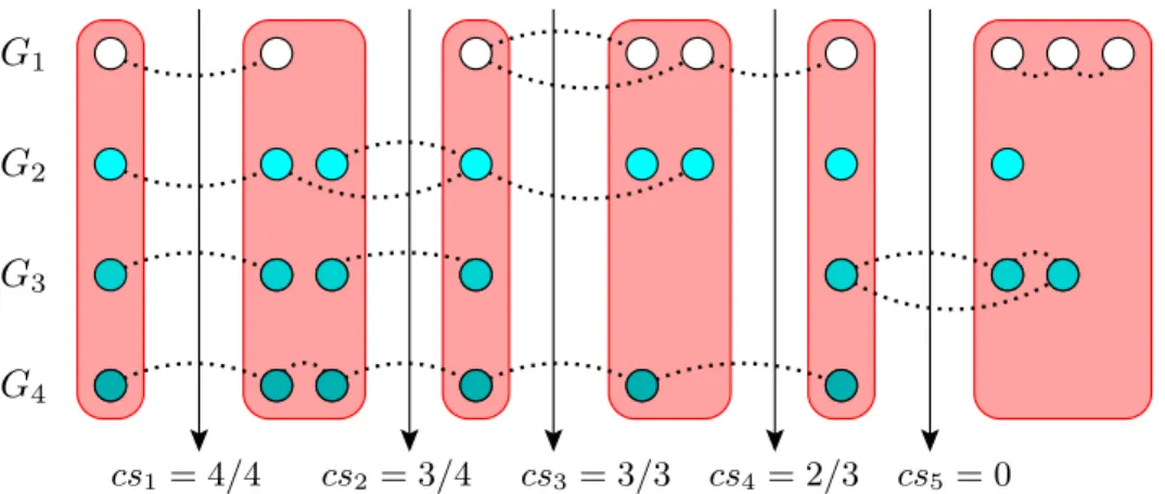
generalization of edge conservation definition of pairwise network alignments. Note that for pairwise alignments edge conservation is assigned a binary value, that is a PPI edge in one network is either conserved in the other network or not. However for multiple alignments the employed definition may assign rational conservation values. We formally define CIQ(CL) as follows: CIQ(CL) = P ∀Clm,Cln P ∀(u,v)∈EClm,Clncs(u, v) P ∀Clm,Cln|EClm,Cln| (2.2)

(24)

cs1= 4/4 cs2= 3/4 cs3= 3/3 cs4= 2/3 cs5= 0

G1 G2 G3 G4

Figure 2.1. Conservation scores on a sample alignment covering all notable cases. For a sample ciq calculation, see Figure 2.1. Note that, rectangular groups represent the clusters of the alignment. The dotted edges represent the protein-protein interactions. Proteins of each PPI network are drawn at separate horizontal layers. The CIQ score for this alignment is (4 × 4/4 + 4 × 3/4 + 4 × 3/3 + 2 × 2/3 + 0)/16 = 0.771.

In Equation 2.1, ICQ(Cli) stands for the internal cluster quality of a given cluster

Cli and is a measure of sequence similarities of involved proteins. Let wmax(u) denote the

maximum weight of any edge incident on u in Sβ. Denote the edge set of Cli with E(Cli).

ICQ(Cli) is defined as follows:

ICQ(Cli) =

P

∀(u,v)∈E(Cli)

w(u,v)2 wmax(u)×wmax(v)

|E(Cli)|

(2.3)

2.2. BEAMS Algorithm

We first show that for a fixedSβ, the global many-to-many network alignment problem

is computationally intractable. Due to clarity considerations we leave the proof to the Chapter 3.

(25)

even for the restricted case where two PPI networks are aligned and all edge weights in Sβ

are equal.

Considering this NP-hardness result, it is necessary to devise efficient heuristics for the problem. Regarding the cluster definition of Equation 2.1 we make the following observation. Each cluster Cli which is a complete c−partite graph, can be subdivided into a set of ni

disjoint cliques, where ni denotes the size of the maximum partition of Cli. In fact, ni

is the minimum possible size for such a set and each clique in the set has size c0 _where

1 ≤ c0 ≤ c. Therefore we view the original alignment problem of being composed of two subproblems: backbone extraction and backbone merging. A backbone is defined as a clique in Sβ and a set of appropriate backbones together form a cluster. The first subproblem is

that of extracting a minimal set of disjoint cliques from Sβ which coversSβ completely and

that maximizes the alignment score AS when each nontrivial clique of size greater than one is considered a cluster in the definition of Equation 2.1. The set is minimal in the sense that no output pair of cliques can be merged together to form a larger clique. Informally, each backbone corresponds to an orthologous set of proteins with at most one protein from each of the input networks. Thus the backbone extraction problem can actually be viewed as the global one-to-one alignment of multiple networks. A group of backbones is called mergeable if their union provides a valid cluster, that is a complete c− partite graph. We define the second subproblem as finding a minimal set of mergeable backbone groups such that no further mergeable group remains and that maximizes the resulting AS score when each mergeable backbone group is considered a cluster in the definition of Equation 2.1. Note that a mergeable group represents a cluster of proteins that are highly homologous since every pair of proteins from different networks are connected by large weight edges in the filtered similarity graph Sβ. Thus imposing the constraint that no further merging can be done on

the set implies the intuition that no two pairwise homologous clusters should be part of the output alignment separately. We show that even these subproblems are computationally hard and we provide efficient heuristics for each one. In what follows, we first present the

(26)

details of Sβ construction, then proceed to provide descriptions of the two main steps of the

BEAMS algorithm.

2.2.1. Construction of Sβ

Considering the sizes of the networks under consideration and the fact that multiple networks constitute the study subject, a suitable filtration on the complete sequence similar-ity graphS is necessary for mainly two reasons. Firstly, even the suboptimal polynomial-time heuristic algorithms require large amounts of computational power as the size ofS increases. Furthermore, taking into account the complete graph S may lead to incorrect alignments as far as biological significance measures are concerned. Most pairs of proteins from different networks do not bear any significance in terms of sequence similarity scores and employing an alignment with the unfiltered similarity graph S may align proteins with almost no ho-mological similarity. As the evolutionary distance between pairs of input networks might be quite different, we employ a relative filtration that takes into account the relative dif-ferences in sequence similarities of pairs of networks. For some user-defined threshold β, we construct the filtered similarity graph Sβ, so that each edge (u, v) is removed from S if

w(u, v) < β × max(u, v), where max(u, v) denotes the maximum of w(u, v0) or w(u0, v) for any u0_{, v}0 _{from the networks of} _{u and v respectively.}

2.2.2. Backbone Extraction

Regarding the first subproblem defined within the BEAMS framework, we show that the backbone extraction problem is NP-hard even for quite a restricted case. The full proof can be found in the Chapter 3.

Proposition 2.2.2. For all values of α 6= 0, the backbone extraction problem is NP-hard even for the restricted case where two PPI networks are aligned and all edge weights in Sβ

(27)

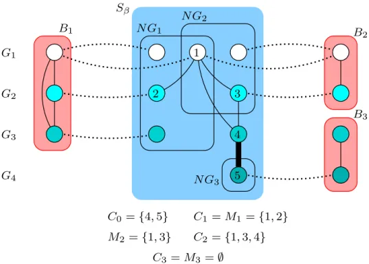
Sβ N G1 N G2 2 3 4 5 G2 G3 G4 G1 1 C0={4, 5} C1= M1 ={1, 2} M2 ={1, 3} C2={1, 3, 4} B3 B2 C3 = M3=∅ N G3 B1

Figure 2.2. Sample neighborhood graph construction and candidate generation for a small instance.

Since the backbone extraction problem is NP-hard, we devise an iterative greedy heuris-tic that runs in polynomial time assuming the number of networks under consideration is con-stant. Our algorithm employs concepts related to maximum edge weighted cliques (MEWC), candidate generation based on neighborhood graph constructions, and a greedy selection heuristic aiming to optimize the AS score. The pseudocode is shown in Algorithm 1.

We start with an empty backbone set and a candidate set that consists only ofC0which

is the MEWC of Sβ. The jth iteration of the main loop of the algorithm consists of four

main steps: Selecting a new backbone Bj among already existing j candidates, removing

the backbone from Sβ, generating the new candidate Cj, and finally updating all existing

candidates. The first step simply involves selecting the new backbone as the candidate providing the maximum AS score when considered together with all existing backbones. Each candidateCj is defined with respect to an already existing backboneBj other than the

(28)

special candidate C0 which is updated throughout iterations as Sβ is updated. To generate

a new candidate Cj via the function call Generate Cand(Sβ, Bj), we first construct the

neighborhood graph of Bj, which is the induced subgraph in Sβ of the set of PPI neighbors

of all the nodes in Bj. If the neighborhood graph does not contain any Sβ edges, then the

candidate Cj is empty. Otherwise, we find the MEWC, Mj, of this neighborhood graph and

we generate Cj by constructing the G-MEWC of Mj in Sβ. Here G-MEWC corresponds

to generalized MEWC which is defined as the maximum edge weighted clique in Sβ that is

required to include all the nodes of Mj; see Figure 2.2 for a sample neighborhood graph

construction and candidate generation on a small instance. In Figure 2.2, the dotted edges represent protein interactions and each network is drawn at a separate horizontal layer. Edges between different layers represent Sβ edges. Besides, the bold Sβ edge between 4 and

5 represents high homological similarity between the corresponding proteins. Candidates are generated with respect to Sβ and backbonesB1, B2, and B3.

Note that on top of the interaction conservation advantages brought by neighborhood graphs, constructing the MEWC of the neighborhood graph guarantees a highly similar backbone candidate as far as homological sequence similarities represented by Sβ edges are

concerned. The G-MEWC construction on the other hand, is a precautionary measure to enable possible extensions of a candidate towards networks other than those of its respective backbone. As the last step within an iteration, we generate each candidate anew, again with respect to its corresponding backbone and the updated Sβ, if it shares any nodes with

the new backboneBj. The iterations continue until Sβ contains only isolated nodes, that is

those of degree zero.

2.2.2.1. Computing Generalized MEWC. We employ a branch-and-bound type algorithm to find the generalized maximum edge weighted clique of Sβ that is required to contain a

given set of nodes, Mj. Note that assigning Mj = ∅, the problem reduces to that of finding

(29)

As is the case with usual branch-and-bound type algorithms, we traverse the search tree T in a depth first manner. Each node at level-i of T represents a clique of size i + |Mj|

in Sβ, that must include nodes in Mj. During the traversal, for each traversed node η =

{u1, . . . , ui+|Mj|} of T representing a clique containing nodes u1, . . . , ui+|Mj|, we store the

neighborhood set of η, denoted with Nη which contains nodes that are in the common Sβ

neighborhood of nodes u1, . . . , ui+|Mj|. The total edge weight of η is denoted with EW (η).

Let Rep(Nη) denote the set of partition numbers of Sβ (the set of PPI networks) that has

a node in the set Nη. Throughout the traversal, we store the best node of the search,

denoted with bestη and its weight with EW (bestη). To complete the description of the

algorithm, we need only to specify the rules for branching and the bound formulation of the search. An upper bound for the potential weight of a node η in T is assigned to, EW (η) +P

∀ut∈η

P

∀r∈Rep(Nη)wmax(ut, r) + P Wmax(Nη), wherewmax(ut, r) denotes the weight

of the maximum weighted edge between ut and any node in the rth partition of Sβ, and

P Wmax(Nη) represents the maximum potential weight of a possible clique inNη. Formally,

P Wmax(Nη) is defined as the sum of the edge weights of the |Rep(Nη)|×(|Rep(N₂ η)|−1) heaviest

edges ofSβ. If the defined potential weight of a nodeη is greater than EW (bestη) we branch

at node η, which implies creating a new node η0 at the next leveli + 1, where η0 = {u1, . . . ,

u_i+|M_j_|, u_i+|M_j_|+1} such that u_i+|M_j_|+1 ∈ Nη.

2.2.3. Backbone Merging

We previously defined the backbone merging problem as finding a minimal set of merge-able backbone groups that maximizes the resulting AS score. With regards to the second main step of the BEAMS algorithm, we first state the following proposition about the com-putational complexity of the corresponding problem. The full proof can be found in the Chapter 3.

Proposition 2.2.3. For α 6= 0, the backbone merging problem is NP-hard even for the restricted case where two PPI networks are aligned and all edge weights in Sβ are equal.

(30)

We provide an iterative greedy heuristic for the backbone merging step. Let M B denote the set of mergeable backbone groups. Initially M B contains all backbones provided by the first backbone extraction step. It is updated at every iteration of the algorithm by a greedy selection strategy which, similar to the backbone extraction step, employs a candidate generation and selection idea. At each iteration we construct all pairs of mergeable groups in M B which all together provide the set of all candidates of that iteration. For each candidate we compute the AS score of M B considering the candidate pair as a single group. Note that some groups in M B may consist of a single node. Such groups are excluded from the AS score computations. We then select the candidate which provides the maximum score and updateM B by merging the pair. The algorithm stops when no mergeable pair remains which provides a minimal setM B. We finally remove groups with a single node and provide the resulting set as the output set of clusters. A full discussion of several implementation details regarding this step and the algorithm as a whole are left to the Chapter 4.

(31)

Algorithm 1 EXTRACT BACKBONES 1: Input: Sβ, G1, G2, . . . , Gk, α

2: Output: Set of backbonesB = {B1, B2, . . . , Bn}

3: B = ∅; C = ∅

4: //Initial candidate

5: C₀ =M EW C(Sβ); C = C ∪ {C0}

6: repeat

7: B_new =Select Cand(C, B); B = B ∪ {Bnew}

8: Remove Bnew fromSβ

9: //Generate new candidate

10: C_new=Generate Cand(Sβ, Bnew);C = C ∪ {Cnew}

11: //Update each candidate in C 12: for all Ci ∈ C do 13: if Ci∩ Bnew 6= ∅ then 14: if i == 0 then 15: C₀ =M EW C(Sβ) 16: else 17: C_i =Generate Cand(Sβ, Bi) 18: end if 19: end if 20: end for

21: until Sβ contains only isolated nodes

22: //Each isolated node is a backbone itself 23: for all nodesu ∈ Sβ do

24: B_new = {u}; B = B ∪ {B_new} 25: end for

(32)

3. NP-HARDNESS PROOFS

In this chapter, we provide the NP-hardness proofs of the propositions in Section 2. The following propositions correspond in the same order to Propositions 2.1, 2.2, and 2.3. All the proofs are based on reductions fromM onotone 1in3SAT which is a restricted version of the 3SAT problem [43]. In Monotone 1in3SAT exactly one literal in each clause is required to be true and none of the clauses contains negated literals.

3.1. NP-Hardness Proof of Global Many-to-Many Alignment Problem

Proposition 3.1.1. For all α 6= 0, the global many-to-many alignment problem is NP-hard even for the restricted case where two PPI networks are aligned and all edge weights in Sβ

are equal.

Proof. Given a Monotone 1in3SAT instance Φ, we show how to construct an instance of the global many-to-many alignment problem that consists of two interaction networks G1, G2

and Sβ the filtered sequence similarity graph. The variable and the clause gadgets are as

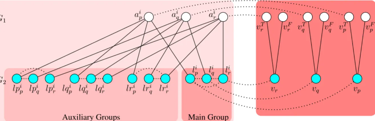
shown in Figure 3.1. Note that each lp node in the auxiliary group is connected to all 6 of the lq and lr nodes of the auxiliary group, each lq node is connected to all 6 of the lp and lr nodes, and finally each lr node is connected to all 6 of the lp and lq nodes. These PPI interactions are not shown in the figure for clarity. The variable gadget corresponding to a variablexp consists of two nodesvpT andvpF inG1, and a single nodevp inG2. Corresponding

to a clause ci = (xp ∨ xq∨ xr) of Φ there are three nodes aip, aiq, air in G1. In G2 12 nodes

are created for the same clause. The nodes li

p, liq, lri make up the main group. Additionally

there are three auxiliary groups, one for each literal in ci. The nodes lpip, lpiq, lpir make up

the auxiliary group for p; lqi

p, lqiq, lqir make up the auxiliary group for q; lrip, lrqi, lrri make up

(33)

Main Group Auxiliary Groups vT p vpF vT q vqF vT r vFr vp vq vr ai p air li p liq lir lpi p lpiq lpir lqpi lqqi lqri lrpi ai q lri q lrri G1 G2

variable gadgets for xp, xq, xr of Proposition 3.1.1.

between its own nodes. In the clause gadget the main group is a K3 in G2. The auxiliary

groups altogether is almost a K9 in G2, except the auxiliary group of p has a missing edge

between lpi

q and lpir, the auxiliary group of q has a missing edge between lqpi and lqir, and

finally the auxiliary group of r has a missing edge between lri

p and lriq. With regards to the

edges between variable gadget nodes and clause gadget nodes, each node vT

p is connected in

G1 to every node ajp for every clause cj such that xp ∈ cj. Similarly in G2, the node vp is

connected to every nodelj

p such thatxp ∈ cj for some clause cj. Regarding similarity edges,

there are edges (vp, vpT), (vp, vpF) in the variable gadget. In the gadget for clause ci, aip is

connected to li

p, lpip, lqpi, lrpi;aiq is connected tolqi, lpiq, lqiq, lriq;air is connected tolri, lpir, lqir, lrir

in the similarity graph. For simplicity we call Sβ edges incident on a main group node a

main group edge and those incident on an auxiliary group node an auxiliary group edge. All similarity graph edges have equal weight.

We show that Φ is satisfiable if and only if the constructed graph admits a global many-to-many alignment with an AS score of 1. Assume Φ is satisfiable. From the variable gadget of a variablexp we choose (vpT, vp) as a cluster if xp is assigned True in Φ and (vpF, vp)

if it is assigned False. For a clause gadget corresponding to ci = (xp ∨ xq ∨ xr), without

(34)

(ai

r, lpir). Note that the nodes aiq, air are clustered with their corresponding nodes from the

auxiliary group of p. The provided clustering is a valid alignment according to the problem definition provided in the section 2.1. We show that with such a clustering the AS score is 1. The ICQ score of each cluster is exactly one since each sequence similarity edge is assumed to have equal weight. We only need to prove that the CIQ score of the output clusters is exactly 1. Note that this corresponds to a cluster selection where the interactions between all cluster pairs are conserved. We only need to show this for a pair that consists of a cluster from a clause gadget and a cluster from a variable gadget, since the clause clusters are chosen so that no PPI edge exists between any pair of clause clusters, and the variable gadget itself contains a single cluster. Both G1, G2 PPI edges connecting to the

cluster (ai

p, lpi) are conserved sinceaip is connected to vpT, lip is connected to vp, and (vTp, vp)

is one of the constructed clusters. The clusters (ai

q, lpiq), and (air, lpir) do not have PPI edges

to variable gadget clusters; (vF

q, vq), (vFr, vr) are their variable gadget clusters and no edge

exists between the pairs ≺ai

q, vqF ≺air, vrF, ≺lpiq, vq, and ≺lpir, vr.

For the reverse direction we show that the existence of a legal alignment withAS score 1 implies the satisfiability of Φ. If such an alignment exists then it must be the case that its CIQ score is also 1, that is every edge between any pair of clusters in the alignment must be conserved. Every G1 node in a clause gadget is neighbors in the similarity graph with nodes

that have a single similarity edge which implies that every G1 node must be involved in a

cluster by the maximality property of a legal alignment. Since the G1 nodes in the clause

gadget do not have any common similarity graph neighbors this further implies that each one must be in a separate cluster and that for every clause gadget there must exactly be three disjoint clusters. We first show that one of these clusters is a main group edge and the other two are auxiliary group edges. Furthermore the auxiliary group edges are incident on nodes that belong to the auxiliary group of the node that the main group edge is incident on.

(35)

Note that there are no three auxiliary group nodes that are pairwise disjoint in G2.

This implies that one of the clusters must involve a main group node for otherwise there would be a G2 edge that is not conserved in G1. Without loss of generality let lip be that

node for the gadget corresponding to the clause ci = (xp∨ xq∨ xr). The clusters of aiq and

ai

r can not include any main group node since that would introduce a nonconserved edge.

Their clusters must then respectively be (ai

q, lpiq), (air, lpir), since among the similarity graph

neighbors of ai

q, air the only auxiliary group nodes that are disjoint in G2 are lpiq and lpir,

and including any other node in the clusters would introduce a nonconserved edge. Note thatlpi

q, lpir are PPI neighbors inG2 with every other node among the auxiliary group. This

implies that the cluster of li

p must be (aip, lpi) since including any other auxiliary group node

that are neighbors ofai

p in the similarity graph would introduce a nonconserved edge.

For the truth assignment ofφ we assign every literal that corresponds to a main edge cluster in a clause gadget to True and every literal that corresponds to an auxiliary edge cluster to False. Thus obviously only one literal per clause is assigned True. We finally need to show that this assignment is a valid assignment in the sense that a variable assigned to True in some clause gadget is not assigned to False anywhere else and vice versa. Let xp be

a variable assigned True due to the main edge cluster selection in a clusterci. It must be the

case that in the variable gadget corresponding to xp the node vTp must belong to a cluster,

for otherwise there would be a nonconserved PPI edge between li

p and vp. This implies xp

can not be assigned False anywhere else due to auxiliary edge clustering, since no auxiliary group nodes are connected to vp in G2 and there would be a nonconserved edge.

3.2. NP-Hardness Proof of Backbone Extraction Problem

Proposition 3.2.1. For all values of α 6= 0, the backbone extraction problem is NP-hard even for the restricted case where two PPI networks are aligned and all edge weights in Sβ

(36)

G

2

G

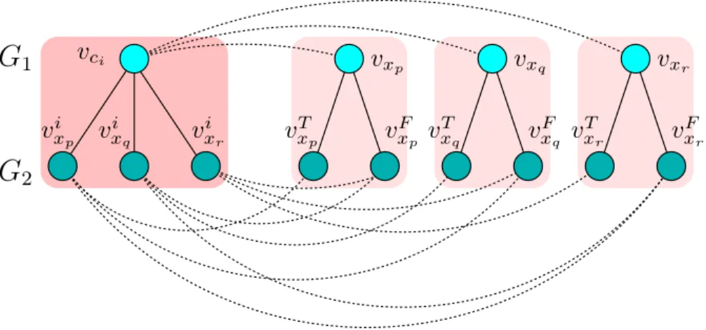
1 vci vi xp v i xq v i xr v T xp vxp vF xp v T xq vxq vxr vF xq v T xr v F xr

Proof. Given a Monotone 1in3SAT instance Φ, we show how to construct an instance of the backbone extraction problem that consists of two interaction networks G1, G2 and Sβ the

filtered sequence similarity graph; see Figure 3.2 for the construction of clause and variable gadgets. For each clause ci of Φ we create a clause node vci in G1. Additionally, for each

variable xp of Φ we create a variable node vxp in G1. For a clause node vci where ci =

(xp∨ xq∨ xr), we create three PPI edges (vci, vxp), (vci, vxq), (vci, vxr) in G1. Corresponding

to each clause node vci of G1 we create three nodes v i xp, v

i xq, v

i

xr in G2. We call these nodes

clause nodes ofG2. Also for each variable nodevxp ofG1 we create two variable nodesv T xp, v

F xp

inG2, each of which is called a literal node ofG2. Each nodevxipofG2is connected with three

PPI edges with vT xp, v

F xq, v

F

xr inG2. The filtered similarity graph Sβ is constructed as follows.

We add three edges betweenvci of G1 and each of its corresponding clause nodes inG2, that

is vi xp, v

i xq, v

i

xr. Additionally we add two similarity graph edges between each variable node

vxp of G1 and the literal nodes v T xp, v

F

xp of G2. Note that all the sequence similarity edges

are assumed to have equal weight. We show that Φ is satisfiable if and only if the AS score of the optimum solution to the backbone extraction problem on the instance G1, G2, Sβ is

exactly 1. Assuming Φ is satisfiable the backbone involving a clause node vci of G1 is the

edge (vci, v i

xp) where xp is the true literal in ci and the backbone involving a variable node

vxt of G1 is the edge (vxt, v T

xt) if xt is assigned True in Φ and it is the edge (vxt, v F xt) if it

(37)

is assigned False in Φ. We show that this assignment of backbones provides a legal output for the backbone extraction problem and that its AS score is 1. It is easy to see that the assignment is legal since the output set of backbones is a minimal disjoint set of cliques. The ICQ score of each backbone is exactly one since each sequence similarity edge is assumed to have equal weight. We only need to prove that theCIQ score of the output backbones is exactly 1. Note that this corresponds to a backbone selection where the interactions between all backbone pairs are conserved. For a backbone (vci, v

i

xp) assigned by the construction, we

show that every edge incident on the backbone be it in G1 orG2 is conserved. The nodevci

is connected to vxp, vxq, vxr in G1 and the node v i xp is connected to v T xp, v F xq, v F xr inG2. Since each of (vxp, v T xp), (vxq, v F xq), (vxr, v F

xr) is also selected as a backbone every edge involving vci

and vi

xp is conserved. Note that considering only the backbones involving clause nodes of

G1, G2 is sufficient since there are no PPI edges between any variable node pair of G1 and

the same is true for any literal node pair of G2.

For the other direction, we show that if there exists a legal backbone extraction that provides an AS score of 1, then we can find an assignment of variables that gives rise to a satisfiable assignment of Φ that is valid with respect to the definition of Monotone 1in3SAT. First we note that every node inG1 must be involved in a backbone due to the full-coverage

condition in the definition of a legal backbone set. Furthermore this backbone cannot be a trivial backbone containing only the node itself for otherwise the backbone set would not be minimal; a clause node in G1 is connected to three nodes from G2 in Sβ which have no

other similarity edges and similarly a variable node in G1 is connected to two nodes from

G2 inSβ which also have no other similarity edges. Given the output backbone set, for each

backbone (vci, v i

xp) involving a clause node of G1 we assign xp True and xq, xr False. First

we show that with this assignment every variable xp is assigned either True or False.

We start by showing that a variable assigned True by a backbone assignment must not be assigned False by the rest of the backbone assignments. In addition to clauseci, letcj be

(38)

another clause containing variable xp. Assuming (vci, v i

xp) is a backbone, we need to show

that (vcj, v j

xp) is also a backbone and thus its assignment of xp does not conflict with that

of the former backbone. We show that the backbone (vci, v i

xp) implies that (vxp, v T

xp is also a

backbone. The variable nodevxp has two candidates for a nontrivial backbone, (vxp, v T xp) and

(vxp, v F

xp). Thus (vci, vxp) is a PPI edge in G1 that must be conserved and this conservation

is only possible by selecting the former backbone candidate sincevi

xp is connected only tov T xp

with a PPI edge inG2. The existence of the backbone (vxp, v T

xp further implies the existence

of the backbone (vcj, v j

xp). This follows from an argument similar to the one above. The

clause nodevcj has three candidates for a nontrivial backbone among which (vcj, v j

xp) has to

be selected as onlyvj

xp has a PPI edge withv T

xp inG2 that conserves the edge (vcj, vxp). Next

we show that a variable assigned False by a backbone assignment must not be assigned True by the rest of the backbone assignments. Assuming (vci, v

i

xq) is not a backbone, we need to

show that there exists no other backbonevcj, v j xq. If (vci, v i xq) is not a backbone (vxq, v F xq must

be a backbone. This follows from the fact that (vci, vxp or (vci, vxr) must be a backbone and

both of vxp, vxr are connected to v F

xq rather than v T

xq in G2. The existence of the backbone

(vxq, v F

xq) implies the nonexistence of (vcj, v j

xq) since there exists no PPI edge (v j xq, v

F

xq) in G2

to conserve the PPI edge (vcj, vxq) of G1. Finally due to the truth value assignment rule,

it is obvious that for each clause exactly one literal is assigned True which implies a valid satisfiable Monotone 1in3SAT instance.

3.3. NP-Hardness Proof of Backbone Merging Problem

Proposition 3.3.1. For all values of α 6= 0, the backbone merging problem is NP-hard even for the restricted case where two PPI networks are aligned, all backbones are 2-cliques and all edge weights in Sβ are equal.

Proof. We similarly construct a reduction from the Monotone 1in3SAT problem. For a given Monotone 1in3SAT instance Φ we provide the construction ofG1, G2,Sβ and the backbone

(39)

bxp bxp bxp b T xp b F xp b T xp b F xp bT xp b F xp axp a T xp a T xq aF xp axq a F xq axr a T xr a F xr ai xr aci a i xq ai xp bci b i xp b i xr bi xq G2 G1

set B. For each variable xp of Φ three nodes axp, a T xp, a

F

xp are created in G1. Corresponding

to each clause ci = (xp ∨ xq∨ xr) we create four nodes aci, a i xp, a

i xq, a

i

xr. The edge set of G1

consists of edges (aci, axt) for each clauseci, where xtis a literal in ci. The node set ofG2 is

similar to that of G1, that is for each variablexp three nodesbxp, b T xp, b

F

xp and for each clause

ci four nodes bci, b i xp, b i xq, b i

xr are created. Regarding the edges of G2, for each clause ci, we

add the edge (bi xt, b

T

xt) for each literal xt ∈ ci and the edge (b i xt, b

F

xw) for each literal pair

xt, xw ∈ ci and xt 6= xw. For each clauseci, we add the following similarity edges: (aci, bci)

and for eachxt∈ ci, (aci, b i xt), (a i xt, bci), (a i xt, b i

xt). For each variablexpthe following similarity

edges are added: (axp, bxp), (axp, b T xp), (axp, b F xp), (a T xp, bxp), (a T xp, b T xp), (a F xp, bxp), (a F xp, b F xp). We

assign a similarity score of 0.5 for each similarity edge. Finally the backbone set B consists of single edges. For each clause ci we have four backbones denoted with clause backbones:

(aci, bci) and (a i xt, b

i

xt) for eachxt ∈ ci. For each variablexp we have three backbones denoted

with literal backbones: (axp, bxp), (a T xp, b T xp), (a F xp, b F

xp). Note that this backbone set includes

all nodes from the input networks and it is minimal, that is no pair of backbones can be merged together to form a larger clique. The construction is illustrated in Figure 3.3.

A key observation is that the maximumCIQ score attainable in any backbone merging of such an input instance is 0.5. This is due to the fact that the cluster backbone (aci, bci)

(40)

can only be merged with only one of (ai xt, b

i

xt) for some xt ∈ ci which further implies that

two backbones in the clause gadget can not be merged with any other backbones. Six G2

edges are incident on those two backbones and none of them can be conserved due to lack of G1 edges incident on them and at most 6 PPI edges out of all 12 in the gadgets involving a

clause and all its literals can be conserved. Thus the maximum AS score achievable in any alignment is 0.5.

We show that Φ is satisfiable if and only if the constructed instance has a back-bone merging that provides a legal alignment with maximum score of 0.5. Assume Φ has a satisfying assignment. For each clause ci, the clusters resulting from mergings is

as {{(aci, bci), (a i xp, b i xp)}, {(a i xq, b i xq)}, {(a i xr, b i

xr)}} where each set in this multiset represents

a set of merged backbones into a cluster and xp is the only variable assigned True in

ci. The clusters resulting from backbone merging in the corresponding variable gadgets

is as {{(axp, bxp), (a T xp, b T xp)}, {(a F xp, b F

xp)}} for the True literal xp and {{(axq, bxq), (a F xq, b F xq)}, {(aT xq, b T xq)}}, and {{(axr, bxr), (a F xr, b F xr)}, {(a T xr, b T

xr)}} for the False literalsxq, xr. Note that

with the provided mergings, the resulting clusters conserve 6 out of all 12 PPI edges from G1, G2between the clusters, when clusters related to a single clause and its variables are

con-sidered. Since every variable has the same truth value assignment in all the clauses, the AS score of the constructed alignment is exactly 0.5, the maximum possible score. Furthermore it is easy to verify that the provided alignment is legal with respect to the main problem definition; each cluster is a complete c−partite subgraph of Sβ for 1< c ≤ 2 and the set of

clusters is maximal, that is no further complete c−partite subgraph remains in Sβ.

For the reverse direction, assume we have a legal alignment withAS score 0.5. In any legal alignment, it should be that for a cluster ci = (xp∨ xq∨ xr), any backbone merging

must include three resulting clusters: {(aci, bci), (a i xt, b

i

xt)} for some xt ∈ ci and {(a i xw, b

i xw)}

for xw ∈ ci and xw 6= xt. We construct a truth value assignment for Φ by considering

(41)

two variables to False. We show that this is a legal Monotone1in3SAT assignment and it evaluates to True.

Since for each cluster exactly one variable is assigned True, it easy to verify that the provided assignment of truth values makes Φ True. It remains to show that this assignment is legal in the sense that a variable xt assigned True due to a clause

gad-get must be assigned True in every clause gadgad-get. As both the AS score and the ICQ score of the alignment is 0.5, it should be that the CIQ score is also 0.5. This im-plies that for every clause gadget and the gadgets involving its variables exactly 6 out of all 12 edges must be conserved, that is all three G1 edges involved in the gadgets must

be conserved. Given a clause ci = (xp ∨ xq ∨ xr), without loss of generality let xp be

the variable involved in merging for the clause gadget of ci, that is the clusters

result-ing from mergresult-ing is as {{(aci, bci), (a i xp, b i xp)}, {(a i xq, b i xq)}, {(a i xr, b i

xr)}}. All three G1 edges

incident on the first cluster must be conserved. To conserve the edge (aci, axp) the

clus-ters resulting from mergings in the variable gadget of xp must be {{(axp, bxp), (a T xp, b T xp)}, {(aF xp, b F

xp)}}. To conserve the edge (aci, axq) the clusters resulting from mergings in the

variable gadget of xq must be {{(axq, bxq), (a F xq, b F xq)}, {(a T xq, b T

xq)}}. Finally, to conserve the

edge (aci, axr) the clusters resulting from mergings in the variable gadget of xr must be

{{(axr, bxr), (a F xr, b F xr)}, {(a T xr, b T

xr)}}. We show that for any clause cj such that xp ∈ cj, it

must be that xp is the variable involved in merging for the clause gadget of cj, that is

the resulting three clusters of cj’s gadget must be {(aci, bci), (a i xp, b i xp)} and {(a i xw, b i xw)} for

xw ∈ ci and xw 6= xp. Assume for the sake of contradiction, xp is not involved in merging

for the gadget of cj, that is one of the resulting three clusters is {(aci, bci), (a i xw, b

i

xw)} for

some xw ∈ cj and w 6= p. Then it is impossible to conserved the edge (acj, axp) incident on

the cluster {(axp, bxp), (a T xp, b

T

xp)} since the cluster is incident on only one G2 edge which is

(bi xp, b

T

(42)

4. IMPLEMENTATION DETAILS AND RUNNING TIME

ANALYSIS

We provide a discussion of BEAMS in terms of its running time requirements and describe implementation details when necessary. The initial preprocessing step of Sβ

con-struction is trivial and requires O(|E|) time where E represents the set of edges in the k−partite graph S.

With regards to the running time analysis of the backbone extraction step described in pseudocode in Algorithm 1 of the Chapter 2, we first provide a description of our im-plementation of finding the generalized maximum edge weighted clique, G-MEWC. Since the input to the G-MEWC algorithm changes throughout the execution of the algorithm we provide a description of the algorithm on a general k0_{−partite graph G}0 _{= (V}0_{, E}0_{) and a}

givenM which denotes the set of nodes required to be in the output maximum edge weighted clique. As a preprocessing step of the G-MEWC algorithm, for each node ut ∈ V0, we first

compute and store wmax(ut, r) for each 1 ≤ r ≤ k0 edges. The preprocessing also includes

the computation of the sum of the weights of the largest r×(r−1)₂ edges. All this information is then employed to speed up the bound calculations; when computing an upper bound for the potential weight of a nodeη of the branch-and-bound tree this preprocessed data is used rather than computing it repeatedly for each tree node. The only remaining information during a bound phase of a nodeη is the common neighborhood of all the nodes stored at η which is computed employing the neighborhood information of η’s parent in the tree. This requires O(∆) time, where ∆ denotes the maximum degree of any node in G0_{. The number}

of nodes of the branch-and-bound tree is bounded by O(|V0|k0

) if M = ∅ and O(∆k0_−|M|

) otherwise, since the common neighborhood ofM can be of size at most ∆. The total running time of G-MEWC is then O(∆|V0|k0

) if M = ∅ and O(∆k0_−|M|+1

) otherwise. Note that the former version of G-MEWC is denoted with MEWC in Algorithm 1.

(43)

Let V denote the set V1 ∪ . . . ∪ Vk. The running time of Algorithm 1 is dominated

by the time spent in the main repeat loop of lines 6 through 21. Note that the number of iterations of the loop is O(|V |), since the maximum number of output backbones can be at most |V |, each iteration finds a new backbone, and the iterations continue until no new backbones remain. The function Select Cand at line 7 finds the candidate that scores the best when considered with the already existing backbone set. Both the new ICQ and the CIQ scores are calculated by computing the contribution of the new backbone and combining this contribution with the existing values. To compute the contribution of theICQ score of a given candidate with the existing backbones requiresO(k2_{) time, whereas the contribution}

to the CIQ score is computed in time O(k2_∆

max), where ∆max is the maximum degree of

any node in V in its respective PPI network. Since the number of candidates at a specific iteration is bounded by O(|V |), the running time required by line 7 is O(|V |k2_∆

max). For

theGenerate Candidate function calls of lines 10 and 17, one call to MEWC is made on the neighborhood graph of the input backbone and one call to G-MEWC is made on Sβ with

the set M containing at least two elements. Note that the size of the neighborhood graph is at most k∆max. The total running time of these two calls is O(∆(k∆max)k+ ∆k−1), where

the first term indicates the time required for the first call and the second term stands for the running time of the second call. Hereinafter ∆ denotes the maximum degree of any node in Sβ, since ∆ gets its maximum value when G-MEWC is called on Sβ. For the calls at

line 15 the set M is empty, thus each call requires the heavier version of G-MEWC, namely MEWC on Sβ which requires running timeO(∆|V |k). Therefore to speed up the algorithm,

we do not actually compute MEWC at each execution of line 15, but rather employ some preprocessing and proceed with updates when necessary. As a preprocessing, the G-MEWC is initially computed for M = {u} for each node u in V and all these G-MEWC sets are stored in a list which requiresO(|V |∆k_{) time in total. At each iteration two main operations}

regarding line 15 are implemented: f ind max and update. The former finds the maximum weighted G-MEWC stored in the current list, whereas the latter recomputes G-MEWC of the nodes in the list that contain nodes already assigned to some backbone. Since each

(44)

iteration of the repeat loop assigns at most k nodes to a new backbone, these nodes can be part of at mostk∆ G-MEWC sets. Thus all the updates at a specific iteration of the repeat loop requires O(k∆) updates each of which requires O(∆k_{) time. In total the running time}

required by line 15 is then bounded by O(|V | + k∆k+1_{)). Note that line 15 is executed only}

once for the update of C0 within the for loop of lines 12 through 20. However line 17 is

executedO(|V |) times since the number of candidates at a specific iteration can be at most |V |. Thus the total running time of the main repeat loop and in turn that of the whole Algorithm 1 is O(|V |2_∆(k∆

max)k+ |V |2∆k−1+ |V |k∆k+1). Assuming ∆max =O(∆) and k

a small constant, which usually is the case for the PPI networks under study, the running time is O(|V |2_∆k+1_).

For the second main phase of BEAMS which consists of backbone merging, assume a backbone list M B is given. We treat M B as a cluster list, iteratively update it, and finally the list remaining at the end of this phase becomes the set of output clusters. First a list of all mergeable pairs of backbones, CM B is constructed. Note that this is done only once,

at the beginning of this phase. Next we iteratively select the best pair from CM B, one that

provides the bestAS score with the rest of the clusters in M B, remove the pair from M B, insert the merged pair back into M B, and update CM B by removing the two candidates

corresponding to the merged pair from CM B and inserting their intersection back into CM B.

Throughout iterations the most time consuming task is that of computing the best pair in CM B. LetCmaxdenote the size of the maximum cluster output by the algorithm. Computing

theICQ contribution of a single candidate requires time O(|Cmax|2). The CIQ contribution

can be computed in timeO(|Cmax∆max|), since this is an upper bound on the total number of

PPI edges incident on the nodes of a candidate. Thus a single execution of this step requires O(|V |2_|C

max|2 + |V |2|Cmax|∆max) time since the number of candidates at each iteration is

bounded by O(|V |2_{). There are} _{O(|V |) iterations in total. Thus the total running time is}

bounded by O(|V |3_C

max|2+ |V3||Cmax|∆max). Note that Cmax is usually a small constant.