Concurrent design of energy management and vehicle stability control algorithms for a parallel hybrid vehicle using dynamic programming

CONTROL ALGORITHMS FOR A

PARALLEL HYBRID VEHICLE USING

DYNAMIC PROGRAMMING

a thesis

submitted to the department of mechanical

engineering

and the graduate school of engineering and science

of bilkent university

in partial fulfillment of the requirements

for the degree of

master of science

By

Halil ˙Ibrahim Dokuyucu

August, 2012

I certify that I have read this thesis and that in my opinion it is fully adequate, in scope and in quality, as a thesis for the degree of Master of Science.

Asst. Prof. Melih C¸ akmakcı (Advisor)

I certify that I have read this thesis and that in my opinion it is fully adequate, in scope and in quality, as a thesis for the degree of Master of Science.

Asst. Prof. ˙Ilker Temizer

I certify that I have read this thesis and that in my opinion it is fully adequate, in scope and in quality, as a thesis for the degree of Master of Science.

Prof. Dr. Hitay ¨Ozbay

Approved for the Graduate School of Engineering and Science:

Prof. Dr. Levent Onural Director of the Graduate School

MANAGEMENT AND VEHICLE STABILITY

CONTROL ALGORITHMS FOR A PARALLEL HYBRID

VEHICLE USING DYNAMIC PROGRAMMING

Halil ˙Ibrahim Dokuyucu M.S. in Mechanical Engineering Supervisor: Asst. Prof. Melih C¸ akmakcı

August, 2012

Concurrent design of controllers for a vehicle equipped with a parallel hybrid pow-ertrain is studied. Our work focuses on simultaneously solving two automotive control problems, energy management and vehicle stability, which are tradition-ally considered separately. The optimal actions for the controllers are obtained by applying dynamic programming using pre-determined drive cycles. By ana-lyzing these actions rule-based controllers are designed so that the results can be implemented on real vehicle controllers. These control algorithms calculate the desired values for the state-of-charge and the wheel slip for the vehicle and this information together with the actual data are used to supervise the subsystem controllers. Our control strategy is based on minimizing the fuel consumption and the wheel slip concurrently. The controller design problems are solved separately also and compared to the concurrent solution. Results show that promising ben-efits can be obtained from the concurrent approach for designing hybrid vehicles which display better fuel economy and vehicle stability.

Keywords: Concurrent Controllers, Hybrid Electric Vehicles.

¨

OZET

PARALEL H˙IBR˙ID ARAC

¸ LAR ˙IC

¸ ˙IN ENERJ˙I

Y ¨

ONET˙IM˙I VE ARAC

¸ DENGE KONTROLC ¨

U

ALGOR˙ITMALARININ ES

¸ ZAMANLI OLARAK

D˙INAM˙IK PROGRAMLAMA YARDIMIYLA

TASARLANMASI

Halil ˙Ibrahim Dokuyucu Makina M¨uhendisli˘gi, Y¨uksek Lisans Tez Y¨oneticisi: Asst. Prof. Melih C¸ akmakcı

A˘gustos, 2012

Paralel hibrid ara¸cların kontrolc¨ulerinin e¸s zamanlı tasarlanması ¨uzerine ¸calı¸sılmı¸stır. C¸ alı¸smamız esas olarak, geleneksel olarak ayrı ele alınan enerji y¨onetimi ve ara¸c denge kontrolc¨u algoritmalarının e¸s zamanlı olarak tasarlanması ¨

uzerine yo˘gunla¸smı¸stır. Optimum sonu¸clar dinamik programlama kullanılarak ¨onceden belirlenen s¨ur¨u¸s ¸cevrimlerinde elde edilmi¸stir. Bu sonu¸cların analiz edilmesiyle ger¸cek ara¸c kontrolc¨ulerine uygulanabilecek kurala dayalı kontrolc¨uler tasarlanmı¸stır. Kontrolc¨uler, ara¸c i¸cin istenen batarya ¸sarj durumu ve ara¸c tek-erle˘gi kaymasını hesaplamakta ve hesaplanan bu de˘gerler ile ger¸cek batarya ¸sarj durumu ve ara¸c tekerle˘gi kayma de˘gerlerini kullanarak alt sistem kontrolc¨ulerini g¨ozetmektedir. Kontrol stratejimizin hedefi, ara¸c yakıt t¨uketimi ve ara¸c tekerle˘gi kayma de˘gerlerinin minimize edilmesi olarak belirlenmi¸stir. Kontrol problemleri ayrı olarak da ¸c¨oz¨ulm¨u¸s olup e¸s zamanlı olarak ¸c¨oz¨ulen kontrolc¨u ile kar¸sıla¸stırma yapılmı¸stır. Elde etti˘gimiz sonu¸clar e¸s zamanlı kontrolc¨uler yakla¸sımının daha iyi hibrid ara¸cların tasarlanmasında faydalar sa˘glayabilece˘gini g¨ostermektedir.

Anahtar s¨ozc¨ukler : E¸s Zamanlı Kontrolc¨uler, Hibrid Elektrik Ara¸clar. iv

First, I would like to thank my advisor Asst. Prof. Melih C¸ akmakcı. He was very helpful and kind during my graduate studies. He took a great role in this thesis. I would also like to thank our department chair Prof. Dr. Adnan Akay. He gave us great support in our academic research.

I would like to thank all the people from the Department of Mechanical Engi-neering at Bilkent University for the great environment of academic life.

Finally I would like to thank my family. They always believed in me and gave their very special support.

Bilkent, August 2012 Halil ˙Ibrahim Dokuyucu

Contents

Acknowledgements v

List of Figures ix

List of Tables xii

1 Introduction 1

1.1 Motivation . . . 1

1.2 Background . . . 2

1.3 Objectives and Problem Statement . . . 5

1.4 Contributions . . . 6

2 Parallel Hybrid Electric Vehicle Model 7 2.1 Parallel Hybrid Electrical Vehicle . . . 13

2.2 Simplified Model Used In Dynamic Programming . . . 15

2.2.1 Vehicle Dynamics Model . . . 16

2.2.2 Powertrain Model . . . 18

2.2.2.1 Transfer Case Model . . . 18

2.2.2.2 Engine Model . . . 20

2.2.2.3 Battery Model . . . 20

2.2.2.4 Electric Motor Model . . . 21

2.2.2.5 Gearbox Model . . . 22

2.3 Complex Nonlinear Model Used In Simulations . . . 23

2.3.1 Vehicle Dynamics Model . . . 23

2.3.2 Powertrain Model . . . 26

2.3.2.1 Transfer Case Model . . . 26

2.3.2.2 Engine Model . . . 26

2.3.2.3 Battery Model . . . 27

2.3.2.4 Electric Motor Model . . . 29

2.3.2.5 Gearbox Model . . . 29

3 Dynamic Programming 32 3.1 Dynamic Programming Overview . . . 32

3.2 Problem Formulation . . . 33

3.3 Implementation in MATLAB . . . 34

3.4 Application to Automotive Control Problems . . . 37

3.4.1 The Concurrent Problem . . . 38

CONTENTS _viii

3.4.3 The Vehicle Stability Problem . . . 45

4 Controller Development 51 4.1 The Vehicle Stability Controller . . . 52

4.2 The Energy Management Controller . . . 56

4.3 The Concurrent Controller . . . 60

5 Conclusions and Future Work 68 5.1 Conclusions . . . 68

5.2 Future Work . . . 70

5.2.1 Real Time Application Aspects . . . 70

5.2.2 Improvement of The Problem Formulation . . . 73

Bibliography 76

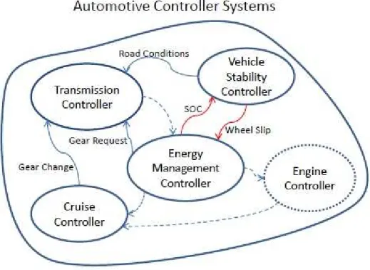
1.1 Automotive Controller Systems Network. . . 3

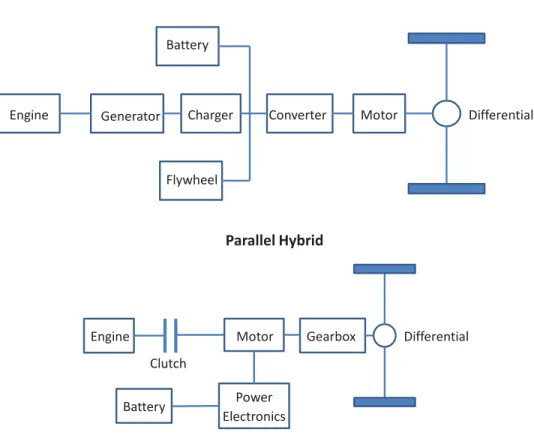
2.1 Series and Parallel Hybrid Vehicle Layouts. . . 8

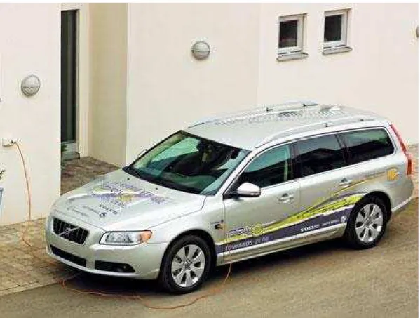
2.2 Volvo V70, a series hybrid vehicle offered by Volvo. . . 9

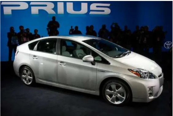
2.3 Toyota Prius, a parallel hybrid vehicle offered by Toyota. . . 10

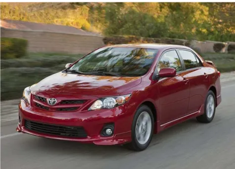
2.4 Toyota Corolla Equipped with VSC System. . . 11

2.5 Configuration of Parallel Hybrid Vehicle. . . 13

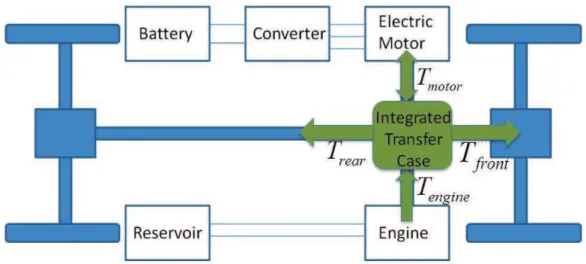
2.6 Integrated Transfer Case Unit. . . 14

2.7 Bicycle model used in [16]. . . 16

2.8 Simulation Model. . . 24

2.9 Vehicle Dynamics Model. . . 25

2.10 Inside the Transfer Case Block. . . 27

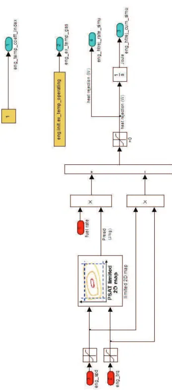
2.11 Thermal Model of the Engine. . . 28

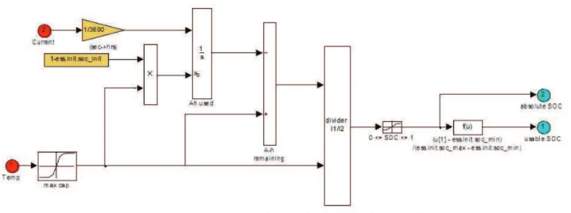
2.12 SOC Algorithm of the Battery Model. . . 29

2.13 Maximum Torque Selection of the Electric Motor. . . 30

LIST OF FIGURES _x

2.14 Speed Calculation of the Gearbox Model. . . 31

3.1 Graphical representation of linear interpolation [5]. . . 36

3.2 Interaction Between Control Problems. . . 39

3.3 FTP 75 Drive Cycle. . . 42

3.4 SOC Behavior of Energy Management Controller. . . 43

3.5 Optimal Operating Points of EM vs Concurrent Controllers. . . . 44

3.6 RRSR Behavior of Vehicle Stability Controller. . . 47

3.7 Optimal Operating Points of VSC vs Concurrent Controllers. . . . 48

3.8 Wheel Slip Comparison of Vehicle Stability and Concurrent Con-trollers. . . 49

3.9 Fuel rate comparison of concurrent and EM controllers. . . 50

4.1 Optimal Traces provided by DP process. . . 52

4.2 Wheel Slip Calculation of the Vehicle Stability Controller. . . 53

4.3 Control Signals of Vehicle Stability Controller. . . 54

4.4 Relationship Between Torque Demand and Wheel Slip. . . 54

4.5 Wheel Slip Behavior of the Vehicle with Vehicle Stability Controller. 55 4.6 Energy Management Controller Add-on Unit. . . 57

4.7 Relationship Between Torque Demand and SOC. . . 58

4.8 SOC Behavior of the Vehicle with Energy Management Controller. 59 4.9 Extracted rules for concurrent controller when wheel slip is high. . 61

4.10 Extracted rules for concurrent controller when wheel slip is low. . 62

4.11 SOC behavior of the concurrent controller. . . 63

4.12 Wheel Slip Behavior of the Concurrent Controller. . . 64

4.13 Fuel rate behavior of the concurrent controller with UDDS. . . 66

4.14 Fuel rate behavior of the concurrent controller with Indian Highway. 67 5.1 Controller Strategy Approach. . . 69

5.2 Signal Process of Concurrent Controller. . . 71

5.3 Signal Processing of the Concurrent Controller. . . 71

List of Tables

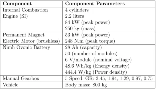
2.1 Vehicle Parameters. . . 12

2.2 Parameters of the Electric Motor. . . 22

3.1 Working Modes of Powertrain. . . 42

3.2 Working Modes of Powertrain. . . 47

3.3 Fuel Consumption and Wheel Slip Comparison over FTP75 Cycle. 48 4.1 Energy Management Controller Rules. . . 58

4.2 Critical Values of SOC and Wheel Slip. . . 60

4.3 Fuel Consumption and Wheel Slip Comparison over UDDS and Indian Highway. . . 66

Chapter 1

Introduction

1.1

Motivation

In parallel with the rapid increase in population around the world, the need for personal mobility and transportation has reached high levels. Although vehicles make our daily life easier, the pollution caused by them is one of the major problems of the big cities and has overall adverse effects to the environment [1]. Automotive companies try to find alternative ways of operating vehicles in cleaner and more efficient ways in order to cope with the strict environmental regulations by the governments. For this purpose engineers have been working on developing promising technologies such as hybrid electric and fuel cell vehicles. However these new vehicles usually result in more complex systems compared to the the vehicles equipped with a conventional powertrain and managing the complexity of such systems with improving the vehicle performance is an ongoing objective for researchers in the automotive field. For example by using hybrid powertrains, which combine two or more power sources in a single system, provides significant improvements in fuel efficiency and reduces the emissions until zero emission vehicle (ZEV) technologies are commercially feasible. However, the inclusion of the new power sources and the accompanying energy storage systems increase the complexity of the system extensively. The operation of today’s vehicles involves

many different controller systems working together with each other in an efficient manner. In Fig.1.1, examples of these controller systems are shown with possible interactions among each other. The principal contribution of this research is the development of a control method that uses the interaction between energy management and vehicle stability controllers. As the interaction between these two problems grows, significant improvements in terms of fuel consumption and wheel slip can be achieved when optimization problems of these controllers are solved concurrently. The strong interaction between the two control problems is presented in Chapter 3. Rules are extracted based on the optimal traces obtained in the Dynamic Programming, DP, process. Results show that when energy management controller is deciding on torque split ratio the information about wheel slip provides more efficient fuel consumption behavior. For instance, the energy loss caused by wheel slip is converted to usable energy by regenerative braking. In addition to this, information about energy management reduces wheel slip values of the vehicle.

1.2

Background

Traditionally, energy management strategies for hybrid electric vehicles are de-veloped considering powertrain dynamics only [9, 6, 4]. Our research shows the benefits of the interaction among the two controller problems which gives us better results when we consider vehicle stability when determining the energy management of the hybrid powertrain or vice versa. We propose concurrent de-sign of two controllers communicating with each other by means of controller area network (CAN) units.

DP is performed in order to obtain the optimal trace of controller outputs given the reference set-point data for the system [15]. The vehicle parameters in this model are updated according to a parallel hybrid vehicle configuration which we have also developed a complex and nonlinear simulation model based on actual vehicle data to be used in the controller development section of our research. Also vehicle longitudinal dynamics of our model is updated according to a bicycle

CHAPTER 1. INTRODUCTION ₃

model, which involves longitudinal dynamics only, including torque split device between front and rear axles in order to be used in developing vehicle dynamics controller algorithm.

There are many studies in literature on the design and performance of en-ergy management and vehicle dynamics controllers. In [8], optimal energy-management strategies for parallel hybrid powertrain of urban buses are studied. The parallel hybrid powertrain model is developed with a one way clutch and au-tomatic transmission. Heuristic control techniques such as logic threshold power split strategy is offered regarding the instantaneously optimized algorithm. The controller proposed in this research tries to minimize the fuel consumption of the vehicle and to make the state-of-charge (SOC) of the battery to stay balanced. The designed controller is mentioned in two steps. First, simple rules arranging the power split between the engine and the electric motor are embedded into the controller architecture and then instantaneously optimization algorithm is applied in order to maximize the controller performance.

Optimal control theory is used when developing the control strategy in the re-search presented in [6]. Two vehicle models are used in this study. First a general complex model is constructed in order to be used in the controller tests over predefined drive cycles. This model is simplified in order to be used in the optimization process. The optimal control theory is applied and an optimization algorithm is obtained. This algorithm is improved by integrating a more accu-rate battery modeling regarding long trips of the vehicle in which the battery may diverge from its nominal values. Computation time for the optimal solu-tion is tried to be reduced in this study. Adaptive control strategy is offered in [17]. Stochastic dynamic programming is used in the development of the control strategy and predictive algorithms are proposed in order to use the controller in real-time applications. The hybrid vehicle is modeled as a stochastic system and the powertrain operation is modeled as a stochastic process. The problem is formulated such that the controller decides on the power split between the engine and the electric motor under the uncertainty conditions. The Markov De-cision Process is used to solve the stochastic problem. The controller results are compared to the ones using the rule-based algorithms.

CHAPTER 1. INTRODUCTION ₅

A vehicle stability enhancement control algorithm is proposed in [9]. The vehicle is modeled as a four-wheel drive hybrid electric vehicle in which there exist two separated electric motors at the rear and the front axles. The benefits of elimi-nating the transfer case unit which splits the total torque between the rear and the front axles are obtained by using separated electric motors. The rear axle is driven only by the electric motor whereas the front axle is driven by both the engine and the electric motor. In the proposed system rear motor control and electrohydraulic brake control is used in order to enhance the vehicle stability during cornering. Also regenerative braking is used in order to improve the fuel economy of the vehicle. Fuzzy logic rules are generated in the proposed control algorithm.

In the thesis presented in [16], simultaneous controller optimization of traction controller for electric vehicles is proposed. Magic Formula is used when modeling the tire longitudinal force which is a function of wheel slip. The controller problem is formulated including continuous and discrete optimization variables so that a genetic algorithm using mixed encoding is proposed in the control strategy development. The optimization process is performed in order to minimize the energy consumed and completion time of a specified drive cycle which has varying surface conditions in the sense of coefficient of friction.

Several methods are offered for developing control strategies of energy manage-ment and vehicle stability controllers. In this thesis we have chosen rule based controllers including optimization by using dynamic programming for our control strategy due to its simplicity and successful examples in many areas.

1.3

Objectives and Problem Statement

In the thesis presented here, the main objective is to show the possible benefits of considering the interaction between the two controllers working in the same physical plant during the design phase. Rule extraction methods are used to obtain nearly optimum hybrid electric vehicle control algorithms compared to

the optimum ones obtained by DP.

Although communication of different controllers via CAN units in vehicle control architecture is well known in literature, our method differs by proposing the problem definition in which we show the interaction between the two control problems by means of the parameter’s selection, i.e. state variables of concurrent controller problem are used in the constant parameters set when defining the single controller problems.

1.4

Contributions

The contributions of this thesis can be listed as follows:

1. An analytical method of solving two automotive control problems concur-rently via DP and developing rule based control algorithms based on the optimal traces gained in DP.

2. A DP for obtaining the optimal traces of the vehicle stability controller and showing that DP works properly in applications of long drive cycles, in contrast to other studies using short profiles with constant road conditions, which have varying road conditions.

3. The integration of a wheel slip model into the hybrid powertrain simulation model which is based on actual vehicle data. Wheel slip and SOC signals network providing the communication between the two control algorithms.

Chapter 2

Parallel Hybrid Electric Vehicle

Model

Hybrid electric vehicles can be classified in two basic powertrain configurations: series hybrid and parallel hybrid. Other configurations which combine series and parallel hybrid features in one powertrain can also be defined. In Fig.2.1, both series (right) and parallel (left) hybrid layouts are described.

In series hybrid vehicles the energy for the electric motor is generated by the engine. The electric motor provides the propelling of the vehicle. As there is no mechanical coupling between the engine and the wheels the optimal operating range of the engine for fuel economy can be achieved most of the time. On the other hand the energy conversion steps between the engine, the electric motor and the wheels result in energy losses of the powertrain. The series hybrid is more efficient during urban driving conditions where the engine speed is expected to vary most of the time. In Fig.2.2, a series hybrid vehicle introduced by Volvo in 2012 is shown. This is a plug-in series model which the battery of the vehicle can be charged off duty by plugging it into any electric source. In the low states of the battery the engine starts to provide power for the vehicle.

In parallel hybrid vehicles the engine and the electric motor are both coupled with the wheels. This coupling is provided by the series of clutches and geartrain,

Series Hybrid

Engine Generator Charger Converter Motor

Battery Flywheel Differential Parallel Hybrid Differential Engine Motor Clutch Battery Power

CHAPTER 2. PARALLEL HYBRID ELECTRIC VEHICLE MODEL ₉

Figure 2.2: Volvo V70, a series hybrid vehicle offered by Volvo. Available from http://www.carpages.co.uk/volvo/volvo-25-09-09.asp.

popularly termed as the power split hardware. They provide the propelling of the vehicle and also assist each other. In low torque demands of the driver the engine has the option to work in high torque level which is more efficient. The extra energy is used to charge the battery and used later. The electric motor has the capability of working as a generator in the braking mode of the vehicle by regenerative braking. The fuel economy benefits of the parallel hybrid configuration are achieved mostly in highway driving conditions. In Fig 2.3, one of the most recognized parallel hybrid electric vehicles commercially available today, Toyota Prius is shown. Toyota introduced the first generation of Prius in 2003. In Toyota Prius continuously variable transmission (CVT) is used in the torque coupling mechanism of the engine and the electric motor as well as in the mechanism of torque transfer to the wheels. Toyota promises to achieve 3.7

and 4.7 [L/100 km] fuel economy values in urban and highway driving conditions respectively. Also 1748 [kg/year] carbon dioxide (CO2) emission is achieved.

Figure 2.3: Toyota Prius, a parallel hybrid vehicle offered by Toyota. Available from http://www.mibz.com/10064-kbbs-green-cars-list-vw-golf-tdi-chevy-tahoe-hybrid-and-others.html.

By definition it is in fact possible to use a parallel hybrid vehicle in series hybrid mode [12]. Researchers try to benefit from the advantages of series and parallel hybrid powertrains at the same time by designing new hybrid powertrain config-urations in which series and parallel hybrid mode is selected by the driver due to the driving condition. When the driver selects the city driving mode the power-train works as a series hybrid and parallel hybrid is activated by the selection of highway driving mode. Seven different parallel hybrid powertrain configurations were studied during the design stage of GM Parallel Hybrid Truck explained in [7]. The design objectives are examined on all powertrain configurations and one specific configuration which shows the best performance is selected.

Vehicle stability control systems are first introduced in the late 1980s by BMW in the name of Electronic Stability Control (ESC). This control system uses the

CHAPTER 2. PARALLEL HYBRID ELECTRIC VEHICLE MODEL ₁₁

Figure 2.4: Toyota Corolla Equipped with VSC System. Available from http://www.autoreview2u.com/toyota-corolla-2011-with-new-interior-car-design/.

engine torque delivery system by reducing the torque provided by the engine in critical conditions. The vehicle stability control systems were taken into account by the automotive producers and rapidly commercialized since then.

In Fig.2.4 new model of Toyota Corolla which uses the latest vehicle stability con-trol (VSC) system developed by Toyota is shown. Skidding condition is detected by the skid sensors of the vehicle and braking or accelerating command is sent through the wheels which need to be adjusted. VSC system also shows control actions during the cornering maneuvers of the vehicle. It prevents the vehicle to get into understeer or oversteer situations.

For the research presented here, we have chosen to work on the parallel hybrid powertrain configuration because of its generality. Since we are studying the coupling effects between energy management and vehicle stability controllers we expect that our results will be more general when the parallel hybrid powertrain configuration is chosen. To this end, we developed a parallel hybrid powertrain

Table 2.1: Vehicle Parameters. Component Component Parameters Internal Combustion 4 cylinders

Engine (SI) 2.2 liters

84 kW (peak power) 250 kg (mass)

Permanent Magnet 53 kW (peak power) Electric Motor (brushless) 248 N.m (peak torque) Nimh Ovonic Battery 28 Ah (capacity)

50 (number of modules) 6 V/module (nominal voltage) 48.6 Wh/kg (Energy density) 444.4 W/kg (Power density)

Manual Gearbox 5 Speed, GR: 3.45, 1.94, 1.29, 0.97, 0.75 Vehicle Body mass: 800 kg

model in Simulink based on actual vehicle data and a typical powertrain config-uration. This is a complex nonlinear plant model based on empirical data from actual vehicles driven by realistic control algorithms which we used as our verifi-cation model as our rule-based vehicle control strategy is developed. This model is presented in section 2.3.

For the DP procedure, a simplified model based on [15] is developed using our complex simulation model vehicle parameters. Longitudinal dynamics of the vehicle are modeled using the bicycle model ignoring the lateral dynamics and the transfer case model in [9] is used to distribute the total torque between front and rear axles. Vehicle component parameters used for our research for both the complex nonlinear and the simplified models are given in Table 2.1. The simple model is suitable for studying both the energy management and vehicle stability problems.

CHAPTER 2. PARALLEL HYBRID ELECTRIC VEHICLE MODEL ₁₃

Figure 2.5: Configuration of Parallel Hybrid Vehicle.

2.1

Parallel Hybrid Electrical Vehicle

We used a typical parallel hybrid electric vehicle configuration with an integrated transfer case as shown in Fig.2.5. The power provided by the electric motor and the power provided by the engine are mechanically coupled in the integrated transfer case unit.

Typical transfer case units split the power between the rear and the front axles. We also integrated the power split mechanism between the electric motor and the engine into the transfer case unit. Total torque demand of the vehicle is met by the electric motor and the engine. Torque Split Ratio (TSR) is the control signal which determines the power split between the electric motor and the engine. Lower level clutch and gearbox control dynamics which handles the transients of the integrated transfer case is assumed to be negligible. That is for example it is assumed that coupling is achieved with no delays.

The integrated transfer case unit also distributes the total power between rear and front axles. Torque Split Factor (TSF) is the control signal which determines the power split between rear and front axles. The torque split between rear and front axles is used to provide vehicle stability during acceleration and braking. In the integrated transfer case unit total torque is mechanically split and transferred to

Figure 2.6: Integrated Transfer Case Unit.

both axles. The physical plant of the integrated transfer case is complicated and has some energy losses during its operation. In Fig.2.6, the integrated transfer case and power split mechanisms are explained.

As shown in Fig.2.6 there are two split mechanisms in the powertrain. Power split between electric motor and engine is determined by energy management controller and torque distribution between front and rear axles is determined by vehicle stability controller. In our proposed controller system the target split levels are controlled at the same time by the concurrent supervisory controller. The engine can operate in more efficient ranges with the help of the electric motor. At high loads the electric motor provides assistance to the engine whereas in low loads the engine can be shut off or works as a generator for the electric motor. In addition, the supervised distribution of the total torque provided to the wheels between the rear and the front axles by the transfer case reduces the wheel slip of the vehicle. Our powertrain model allows us to control the power split between the electric motor and the engine and torque distribution between the rear and the front axle at the same time.

CHAPTER 2. PARALLEL HYBRID ELECTRIC VEHICLE MODEL ₁₅

used here. One possible configuration is that the rear axle is propelled by the en-gine while the front axle is propelled by the electric motor. In this configuration, the power split decision between the engine and the electric motor needs to inter-act with the power split decision between the rear axle and the front axle in such a manner that control signals of the power split mechanisms are not separated from each other.

For another possible configuration, there are two electric motors mounted on each axles and the engine providing power for each axle. In this configuration, transfer case unit is used for only the power split of the engine between rear and front axles while two mechanical coupling units in each axle are needed for the power split mechanisms between the engine and the electric motor.

In our research, we use more general powertrain configuration rather than specific configurations. The results of our research presented in this thesis are generic enough so that they can be extended to specific powertrain configurations easily.

2.2

Simplified Model Used In Dynamic

Pro-gramming

Our simulation model is based on empirical data from actual vehicles which has many numbers of dynamic states and high level of complexity. This model is a useful tool for calculating the validity of the controllers using heuristic control techniques such as rule extraction [16].

As mentioned earlier dynamic programming (DP) is also used in the research pre-sented in this thesis. The performance of DP is highly related with the accuracy and the number of states of the model used for DP. Nonlinear models result in inaccuracy and the computation burden of the process is high.

For the DP procedure, a simple but functional mathematical model is preferred rather than a complex nonlinear model. The dynamic states of the complex nonlinear model are degraded based on the simplification methods introduced in

Figure 2.7: Bicycle model used in [16].

[15]. The simplified model is left with two dynamic states, namely SOC and the wheel slip. Based on the characteristics of the DP, which is explained in detail in Chapter 3, these dynamic states are used individually or together in the model. The components that take part in the simplified hybrid vehicle model are ex-plained in the sections 2.2.1-2.2.2.

2.2.1

Vehicle Dynamics Model

The vehicle dynamics are modeled using the bicycle model without the lateral dynamics. Dynamic weight transfer between front and rear axles is considered due to the vehicle acceleration. The model used in [16] is followed. The bicycle model used in this study is shown in Fig.2.7.

The inputs of the vehicle model are vehicle velocity, vveh, and vehicle acceleration,

aveh. Predetermined drive cycle data in forms of vehicle velocity and acceleration

CHAPTER 2. PARALLEL HYBRID ELECTRIC VEHICLE MODEL ₁₇

As this is a bicycle model including the longitudinal dynamics only, vehicle mass is modeled as the half of the total vehicle mass. At the contact points between tires and the road there are the reaction forces, Fz1 and Fz2, due to the gravitation, g:

Fg = mg = Fz1+ Fz2 (2.1) where Fz1 = mg l1 l , Fz2 = mg l2 l . (2.2)

Longitudinal tire forces are produced with propulsion or braking action of the vehicle. There is a linear relationship, shown in equation (2.3), between the tire normal forces, obtained in equation (2.2), and maximum tire longitudinal forces Fxi,max, which limits the tire friction forces. The road friction coefficient µ, is

assumed to be uniform. In equation (2.3), Fxi denotes the actual friction forces

between the tire and the road.

|Fxi| ≤ |Fxi,max| = µFzi for i = 1, 2 (2.3)

The drag force as a function of vehicle velocity, v, and drag coefficient, C, can be described as

Fdrag = Cv2. (2.4)

By using Newton’s second law we can find the relationship between the vehicle acceleration and the longitudinal tire force.

aveh =

Fx1+ Fx2

m = Fx

m (2.5)

where Fx is the net external longitudinal tire force and it is limited by the front

and rear maximum longitudinal tire forces as

|Fx| ≤ |Fx1,max| + |Fx2,max| = µ(Fz1+ Fz2) = µFg. (2.6)

With equations (2.5) and (2.6) we can obtain a limit for the acceleration. The condition for this limitation is given as

Before analyzing the tire normal forces the longitudinal dynamics can be written as a static system by considering d’Alambert’s Principle

Fx+ FL = 0 (2.8)

where FL denotes the inertial force associated with accelerating/decelerating

sta-tus of the vehicle in the above equation. By using equations (2.5) and (2.8) FL

is found as

FL = −maveh. (2.9)

Weight transfer under vehicle acceleration is modeled as Fz1 = Fg l − l1 l + FL× h l , (2.10) Fz2 = Fg l1 l − FL× h l (2.11)

where Fz1 and Fz2 denote the vehicle traction forces of the front and the rear

wheels respectively. Fg represents the weight of the vehicle and FL represents

the inertial forces of the vehicle. l is used for the distance between the axles of the vehicle whereas l1 is used for the distance between the center of gravity of

the vehicle and the front axle. h is used for the height of the center of gravity of the vehicle. In equations (2.10)-(2.11) first terms on the right hand represent the static weight distribution and second terms represent the dynamic weight distribution.

2.2.2

Powertrain Model

2.2.2.1 Transfer Case Model

As discussed before rear and front axle torque values can be different from each other while providing the vehicle traction stability. In order to distribute the torque between front and rear axles we need to use a mechanical accessory like a center differential. There exists complex transfer case models such as those used in [4] but for simplicity we used a zero order model as in [9]. The inputs of the

CHAPTER 2. PARALLEL HYBRID ELECTRIC VEHICLE MODEL ₁₉

model are the total torque produced, inertia, rotational speeds of the front and rear axles. The outputs are the torque values of front and rear axles.

Output torque is calculated as

Tout = ratio × Ti. (2.12)

Front and rear torque values are determined via factor of torque split, (K), as shown below:

Tout,f ront = Tout× Kf ront, (2.13)

Tout,rear = Tout× Krear. (2.14)

Factor of torque split, Krear, is a function of rear rotational speed ratio (RRSR),

ωratio,rear which is calculated as

ωratio,rear = 0.5 +

ωrear − ωf ront

0.5 × (ωrear+ ωf ront)

. (2.15) In equation (2.15), ωrear and ωf ront denote the rear axle and front axle

rota-tional speeds respectively. In practice, the control law uses wheel slip instead of ωratio,rear. It should be noted that wheel slip is a function of ωratio,rear:

wheel slip = ωratio,rear− 0.5. (2.16)

The function, f (ωratio,rear), is to be the control law of the vehicle stability

con-troller.

Krear = f (ωratio,rear) (2.17)

RRSR is the dynamic state of the model and it depends on the speed difference of front and rear axles. This ratio is the function of the wheel slip of the vehicle and the objective of the vehicle stability controller is to make the RRSR value at 0.5, i.e. zero slip.

The split factors of rear and front axles sum up to unity:

The output rotational speed is calculated as

ωin = ratio × ωout. (2.19)

ratio denotes the reduction in the transfer case model and it is unity, i.e. the rotational speeds of the electric motor and the engine are assumed to be the same.

The mean value of the rotational speeds of front and rear axles, ωout, which is

defined in equation (2.20), which appears in equation (2.19).

ωout =

(ωrear+ ωf ront)

2 (2.20)

2.2.2.2 Engine Model

A quasi-static model is used for the engine. The static map obtained from the actual vehicle data determines fuel consumption rate.

Quasi-static model consists of a steady state model to which an equivalent dy-namical model of the system is added. The output torque of the engine is modeled as

Tengine,out= Teng−

Ploss,eng

ωeng

. (2.21)

Here Ploss,eng represents the frictional losses of the engine. Ploss,eng is assumed to

be a constant average value whereas in complex model it is assumed to be varying with respect to the engine speed. Constant fuel rate is assumed during the idling.

2.2.2.3 Battery Model

The open circuit voltage of the battery,Voc, is governed as

Voc=

qbatt

Cbatt

CHAPTER 2. PARALLEL HYBRID ELECTRIC VEHICLE MODEL ₂₁

Here qbatt represents the charge of the battery. The capacitance of the battery,

Cbatt, depends on the internal temperature and current of the battery.

SOC of the battery is modeled as a normalized value, which represents the charge capacity of the battery

SOC = Voc− Vmin Vmax− Vmin

(2.23) where Vmin and Vmax represent the minimum and maximum allowable voltage

of the battery. These minimum and maximum values are selected as 250V and 400V respectively based on the electric motor used in the modeling.

The provided voltage of the battery can be shown as

Vout = Voc− ibattRbatt (2.24)

It should be noted that transients and thermal effects are neglected. So the only dynamic state is SOC value of the battery.

2.2.2.4 Electric Motor Model

Electric motor dynamics are faster than battery dynamics. The motor model developed does not have a dynamic state. The losses of the motor are taken into account considering the output torque and speed.

The power needed by the motor is a mapped function of output torque, Tmot, and

speed, ωmot

Pbatt = Pmap,motor(Tmot, ωmot). (2.25)

The maximum allowable current of the motor, imax,mot, limits the maximum

elec-tric power, Pmax,mot, supplied from the motor

Pmax,mot= imax,motVout. (2.26)

The mechanical torque limit of the motor, Tmax,mech , is given as

Table 2.2: Parameters of the Electric Motor. Parameter Value

imax,mot 475 A

Pmax,mot 53kW

ωmax,mot 8000 rpm

Here peak torque value of the motor, Tpeak(ωmot), and the continuous torque

value of the motor, Tcont(ωmot), are the mapped functions of rotational speed of

the motor, ωmot. The heat index HI appeared in the above equation arranges

the available torque between the peak and the continuous torques during its operation.

The maximum allowable electrical power available to the motor and the motor speed also limit the output torque. Maximum allowable output torque of the motor limited electrically, Tmax,elec, is

Tmax,elec = Pmap,motor−1 (Pmax,motor, ωmot) (2.28)

where P−1

map,mot represents the inverse map of the motor. In Table 2.2 limitation

parameters of the electric motor are given.

2.2.2.5 Gearbox Model

Gear ratio, GT, and loss terms, Tloss,gb, are considered when modeling the gearbox.

The torque passing through the gearbox, Tgb, can be described as

Tgb = GT × (Tout,tc− Tloss,gb) (2.29)

where Tout,tcrepresents the output torque of the transfer case. The gearbox losses,

Tloss,gb , are assumed to be constant.

Wheel torque, Twheel, is described with final drive ratio, gf, output torque of the

gearbox, Tout,gb, and loss terms of the final drive, Tloss,f d, included as

CHAPTER 2. PARALLEL HYBRID ELECTRIC VEHICLE MODEL ₂₃

2.3

Complex Nonlinear Model Used In

Simula-tions

In our controller development stage of research we developed a complex and non-linear simulation model in Matlab\Simulink environment based on actual data. For developing this model Autonomie simulation software which is based on the several actual vehicle and component tests of Argonne National Laboratory are taken as the reference point when developing our simulation model which is driven by realistic controllers. We configured our model by selecting the appropriate model blocks from the libraries of Autonomie. The original controller blocks are upgraded according to the control algorithms we developed which will be explained in detail in the controller development section.

In Fig.2.8, the high level model blocks representation of our complex nonlinear simulation model is given. Two power paths provided by the engine and the electric motor are separated. The total torque is obtained by summing up the torques provided by the engine and the electric motor. The total torque is then distributed to the rear and the front axles via the integrated transfer case unit. The model blocks of the rear and the front axles are separated from each other as shown in the above figure. The outputs of the powertrain are collected by signal processing blocks and feed the controller blocks.

2.3.1

Vehicle Dynamics Model

Vehicle dynamics model is separated to rear and front axle dynamics including the bicycle model ignoring the lateral dynamics. Vehicle dynamics model is di-vided into three subblocks, namely differential block, wheel block and axle block. Output torque of the transfer case is the input and the vehicle speed is the output of the vehicle dynamics model. The system is fed by the control signals of energy management and vehicle stability controllers. These signals are processed by the wheel model.

CHAPTER 2. PARALLEL HYBRID ELECTRIC VEHICLE MODEL ₂₅

In Fig.2.9, the model blocks providing the vehicle dynamics are shown. Since the vehicle longitudinal dynamics are modeled only steering angle is neglected in the wheel model. The tire forces generated by cornering are excluded in the model. It should be noted that control signals are used in the wheel models. In wheel model a feedback traction controller is embedded using the control signals. This traction controller will be explained in detail in section 4.3.

2.3.2

Powertrain Model

Powertrain model includes two power paths adding up in the transfer case. As this is a mathematical model summation is done before the gearbox block in our simulation model. Controller blocks feed the powertrain during its operation.

2.3.2.1 Transfer Case Model

The transfer case is modeled as having an input of the total output provided by the electric motor and the engine and giving an output of the distributed torque to the axles. Front and rear wheel speeds values drive the mechanism of determining the power split between rear and front axles.

Fig.2.10 shows the model block representation of the integrated transfer case unit. The weighted speed of the rear and the front axles is calculated by taking the mean value of the sum of the rear and the front axle speeds. Rear rotational speed ratio is calculated via a specific function. The rear and the front torque ratio values are calculated by a look-up table embedded into the integrated transfer case unit.

2.3.2.2 Engine Model

When modeling the engine Autonomie map functions are heavily used in calcu-lation steps of engine torque, fuel rate, exhaust emissions. Thermal model of the engine is also embedded in the engine model.

CHAPTER 2. PARALLEL HYBRID ELECTRIC VEHICLE MODEL ₂₇

Figure 2.10: Inside the Transfer Case Block.

In Fig.2.11, the model block representation of the thermal model of the engine is given. The heat rejection characteristics of the engine is calculated based on the actual values of the engine speed, the engine torque and the fuel rate.

2.3.2.3 Battery Model

Battery model consists of voltage and SOC calculation based on mapped func-tions. Temperature effects are also included in the model. SOC algorithm highly depends on the temperature effects of the battery.

The calculation process of SOC value of the battery is shown in Fig.2.12. A look-up table determines the maximum power capacity of the battery with respect to the temperature value of the battery. This maximum power capacity and the consumed power values are used in the calculation process of the SOC.

CHAPTER 2. PARALLEL HYBRID ELECTRIC VEHICLE MODEL ₂₉

Figure 2.12: SOC Algorithm of the Battery Model. 2.3.2.4 Electric Motor Model

Battery voltage is the main input to the electric motor model. Torque provided by the electric motor which is driven by the control signal of power split between the electric motor and the engine is the output. In Fig.2.13 the maximum torque selection model block is represented. Peak and continuous torque values for pro-pelling and the regenerative modes of the electric motor are determined based on the look-up tables using the actual speed of the electric motor. There is a switch mechanism between propelling and the regenerative modes based on the control signal of the electric motor. Heat index HI is calculated in subsystem using the actual and the continuous torque values of the electric motor. The maximum torque selection process decides on whether the torque is limited mechanically or electrically.

2.3.2.5 Gearbox Model

Gearbox model gets the gear number information from the original controller blocks of Autonomie including the gear shifting strategy. As the appropriate

CHAPTER 2. PARALLEL HYBRID ELECTRIC VEHICLE MODEL ₃₁

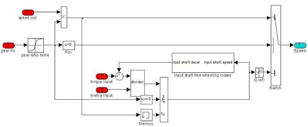
Figure 2.14: Speed Calculation of the Gearbox Model.

gear number is determined speed and torque calculation are done in the model. Gear table based on our vehicle parameters is entered into the model. Speed calculation process of the gearbox is shown in Fig.2.14. It should be noted that the free wheeling losses of the gearbox is modeled and used in the model when the gear number of the vehicle is zero.

Dynamic Programming

Dynamic Programming (DP) is a design optimization tool which can be applied to systems with defined design objectives. It is applied in a number of areas such as information theory, bioinformatics, computer science and control theory [3]. In control theory, DP is used for obtaining the optimal outputs of controllers to be designed [13].

3.1

Dynamic Programming Overview

Bellman’s principle of optimality constitutes the basics of DP. According to Bell-man’s principle, the optimality of subsequent control actions included in the main optimization problem should be validated on the entire space defined for the prob-lem with respect to the resulting state of the first decision of the sequence. This optimal behavior is independent of the initial conditions of the system [2]. The optimal trajectories of subproblems build up the optimal trajectory of the main problem. The performance of the DP process depends highly on the dynamic states defined for the problem. The number of the states directly affects the computation burden and the memory needed for the DP process.

CHAPTER 3. DYNAMIC PROGRAMMING ₃₃

3.2

Problem Formulation

In order to formulate the problem to be solved with DP, continuous time models should be discretized first as shown in (3.1).

xk+1 = f (xk, uk, k) (3.1)

Here xkrepresents the state vector of the system, ukrepresents the control actions

of the system and k represents the time instant of the DP process. After the model is discretized for numerical optimization, a general DP problem is stated [2, 5]:

A general DP problem

given an objective J, solve min J = N X k=0 L(xk, uk, k) (3.2) where xk+1 = f (xk, uk, k) (3.3) subject to x ∈ Xk ⊂ Rn, u ∈ Uk ⊂ Rm. (3.4)

In 3.2-3.4 N denotes the length of the drive cycle. L is defined as the cost function of a single subsequent stage whereas J represents the total cost of the system. Constraints on system states, Xk, and control actions, Uk, can also be defined as

shown in equation (3.4). The constraints of the system are stated as shown in equation (3.5).

Xk : xmin ≤ xk ≤ xmax (3.5)

Uk : umin ≤ uk ≤ umax

xmin and xmax represent the minimum and maximum allowable values of the

system states respectively. umin and umax represent the minimum and maximum

allowable values of the control actions respectively.

The general DP problem defined in equations (3.2)-(3.4) can be solved by numer-ical methods according to the Bellman’s principle of optimality [11].

In equations (3.6)-(3.7), Jk represents minimum cost function between the stage

k and stage N . The problem formulation is shown as if it is starting from the state of xk. Jk(xk) = _umin k,...,uN   N X j=k L(xj, uj, j)   = min uk  L(xk, uk, k) + min uk+1,...,uN   N X j=k+1 L(xj, uj, j)     (3.6) = min uk [L(xk, uk, k) + Jk+1(xk+1, k + 1)] where JN(xN) = min u(N )[L(xN, uN, N )] (3.7)

3.3

Implementation in MATLAB

In our research we used the DP algorithm outlined in [14] with appropriate mod-ifications based on our parallel hybrid vehicle model. In this section the DP algorithm in [14] is summarized. As the result of the research presented in [14] a generic Matlab function which solves deterministic optimization problems specif-ically for energy management strategy of parallel hybrid vehicles is developed. First the optimization problem is defined as outlined in equations (3.2)-(3.4). Continuous time model is discretized according to the equation (3.1).

Control policy, π, is defined as a function of control actions, µi,as

π = µ0, µ1, . . . , µN −1. (3.8)

The discretized cost function is rearranged as shown in equation (3.8) based on the control policy defined in equation (3.7) where initial state is defined as, x(0) = x0.

Jπ(x0) = gN(xN) + ϕN(xN) + N −1

X

k=0

hk(xk, µk(xk)) + ϕk(xk) (3.9)

In equation (3.9) gN(xN)+ϕN(xN) stands for the final cost in which an additional

penalty function is defined within as, ϕN(xN), which has an effect on the final

CHAPTER 3. DYNAMIC PROGRAMMING ₃₅

control actions of µk(xk). Another penalty function, ϕk(xk), which has an effect

on system state constraints.

An optimal control policy is defined as shown in equation (3.10). J0(x0) = min

π∈ΠJπ(x0) (3.10)

Here the control policy is minimized over a finite horizon. Π stands for the all possible control policies.

The DP algorithm calculates the optimal cost-to-go function at every stage going backwards based on the Bellman’s principle of optimality as discussed earlier.

Jk(xi) = min uk∈Uk h hk(xi, uk) + ϕk(xi) + Jk+1(Fk(xi, uk)) i (3.11) Linear interpolation is used to calculate the cost-to-go function, Jk+1(Fk(xi, uk)).

The interpolation procedure is represented graphically in Fig.3.1.

The optimal control signal map is obtained as the result of the discretized cost function defined in equation (3.8). The optimal trajectory of the controller is obtained using this optimal signal map during the forward simulation of the model. It should be noted that the optimal cost-to-go function defined in (3.10) is calculated on the discretized points of the specified state space. However the function Fk(xi, uk) which is included in the last term of the optimal

cost-to-go function is a continuous function. When the output of this function stays between any two nodes on the state space the optimal cost-to-go function should be calculated with suitable approximation methods. Linear interpolation is used for the control signal when actual state does not match the discrete points. Detailed description on how to use the “dpm function” which solves the dis-cretized optimal control problem is given in [14] and also in the appendix. The structure of the function is given as:

[res dyn] = dpm[f un, par, grd, prb, options]

Here f un stands for handling the dpm function, par is the parameter structure defined by the user, grd is the grid structure, which is constituted by the nodes on

CHAPTER 3. DYNAMIC PROGRAMMING ₃₇

which the discretized optimal cost-to-go function is solved, defined by the user, prb is the problem structure and options is the option structure selected by the user. As the output of the dpm function, two variable structures are created: output of the DP procedure and the optimal signal trajectory calculated using the control signal map.

3.4

Application to Automotive Control

Prob-lems

In the research presented in [14] an automotive optimization control problem is given as an example. A Quasi-static discrete-time model of an hybrid vehicle is used to define the fuel consumption of the vehicle. SOC of the battery is chosen as the only state variable of the model. The details of the mathematical modeling of the vehicle components are given in [14].

The discretized model is defined based on the model equations as described in equation (3.12).

xk+1 = f (xk, uk, vk, ak, ik) + xk (3.12)

In equation (3.12) xk denotes the SOC of the battery which is the only dynamic

state of the model, uk denotes the control signal of the model which is defined as

the torque split between the engine and the electric motor, vk, ak, ik, denote the

vehicle speed, vehicle acceleration and the gear number of the vehicle respectively at the instance of k. As vehicle speed, vk, vehicle acceleration, ak, and the gear

number, ik, are known by the drive cycle defined for the system, the discretized

model defined in equation (3.12) can be reduced to a simplified model:

xk+1 = f (xk, uk) + xk, k = 0, 1, 2, . . . , N − 1. (3.13)

In equation (3.13), k denotes the instance of the calculation steps. The simulation time is set up by defining the end point of instance which is denoted as N .

Optimization control problem of the hybrid vehicle

Given an objective J, solve min uk∈Uk J = N −1 X k=0 ∆mf(uk, k) · Ts (3.14) where xk+1 = f (xk, uk) + xk (3.15) subject to x0 = 0.55, xN = 0.55, xk ∈ [0.4 0.7] (3.16) and N = 660 Ts + 1 (3.17)

Through the equation (3.14)-(3.17), the fuel consumption of the vehicle is denoted by the function, ∆mf(uk, k).Ts. Time step, Ts is selected as Ts = 1s. The state

space of the state variable is given in equation (3.16). The number of calculation step is calculated as considering the period of the drive cycle. In the research presented in [14] Japanese 10-15 (J1015) drive cycle is used.

The optimal control problem formulated in equations (3.14)-(3.17) is solved using

dpm function.

In sections 3.4.1-3.4.3 the automotive control system design problems for our research using DP are described.

3.4.1

The Concurrent Problem

Since the concurrent control system is the main focus in our research, control systems for energy management and vehicle dynamics are presented concurrently first. In Fig.3.2 the interaction between the two control problems are explained. The two dynamics states, SOC and RRSR, are used together in concurrent prob-lem formulation. These dynamic states communicate with each other during the DP procedure. The optimal solution of energy management problem at each

CHAPTER 3. DYNAMIC PROGRAMMING ₃₉

Figure 3.2: Interaction Between Control Problems. instance is used when the vehicle stability is solved and vice versa.

This relation outlined in Fig.3.2 is stated in equations (3.18)-(3.20) in which the optimization control problem for concurrent controller is formulated for two dynamic states, namely SOC and RRSR.

The concurrent DP problem

Given an objective J, solve min T SRk∈Uk1(x 1 k),T SFk∈Uk2(x 2 k) J = K−1 X k=1 n fHEV,k(x1k, T SRk), fvehicle,k(x2k, T SFk), k o (3.18) where x1_k+1 = f (x1k, u1k) + x1k, k = 0, 1, . . . , N − 1 x2 k+1 = f (x2k, u2k) + x2k, k = 0, 1, . . . , N − 1 (3.19) subject to x1k ∈ Xk1 ⊂ [0.4 0.7], u ∈ Uk1 ⊂ [−1 1] x2_k ∈ X_k2 ⊂ [0.3 0.7], u ∈ U_k2 ⊂ [0 1] (3.20)

3.4.2

The Energy Management Problem

The objective of the energy management controller problem is to minimize the fuel consumption of the vehicle over a predefined drive cycle. A quasi-static discrete-time model is used to define the fuel consumption of the vehicle. Our energy management DP formulation is similar to the one presented in [14]. The SOC is the only dynamic state in the model. And torque split ratio between internal combustion engine and electric motor is the control signal. In [14], the discrete model is firstly defined as

x1_k+1= f (x1_k, u1_k, v, a, i) (3.21) where x1

kstands for SOC, u1kstands for torque split ratio between internal

combus-tion engine and electric motor, v stands for vehicle velocity, a stands for vehicle acceleration and i stands for gear number.

CHAPTER 3. DYNAMIC PROGRAMMING ₄₁ x1_k+1 = f (x1_k, u1_k), k = 0, 1, . . . , N − 1 (3.22) where x1_k ∈ S_k1 ∧ u1_k ∈ C_k1 (3.23) with S_k1 = [0.4 0.7] ∧ C_k1 = [−1 1] (3.24) N denotes the number of calculation steps in the DP procedure based on the length of the drive cycle defined for DP procedure. S1

k and Ck1 are defined as the

state space and input space for the dynamic programming algorithm respectively in equation (3.24). S1

k limits the dynamic state of the model, and Ck1 limits the

control signal of the controller. Here it is assumed that driving cycle is known in advance. In our study FTP75 drive cycle is used for all simulations in order to have a fixed basis when comparing different controller schemes. Fig.3.3 shows the velocity profile of the FTP75 drive cycle.

The optimization problem for energy management controller is formulated as below.

The energy management DP problem

Given an objective J, solve min T SRk∈Uk1(x 1 k) J = K−1 X k=1 fHEV,k(x1k, T SRk) (3.25) where x1_k+1 = fHEV(x1k, T SRk) (3.26) subject to x1k∈ Xk1 ⊂ [0.4 0.7], T SRk∈ Uk1 ⊂ [−1 1]. (3.27)

In equation (3.25), fHEV(x1k, T SRk) is the fuel consumption function of the HEV

model as a cost of the system. fHEV(x1k, T SRk) calculates the fuel consumption

of the vehicle as

0 200 400 600 800 1000 1200 1400 1600 1800 2000 0 5 10 15 20 25 30 TIME (sec) Vehicle Velocity (mph) FTP 75 Drive Cycle

Figure 3.3: FTP 75 Drive Cycle. Table 3.1: Working Modes of Powertrain. TSR RANGE WORKING MODE T SR = 0 Electric Motor Only Mode 0 < T SR < 1 Torque Assist Mode T SR = 1 Engine Only Mode 1 < T SR Battery Charging Mode

Dynamic state, x1

k, is SOC and control signal, T SRk, is torque split ratio between

internal combustion engine and electric motor. The objective of the DP algorithm is to minimize the cost function.

TSR is defined as

T SR = Engine T orque Calculated at the W heels

T otal T orque Calculated at the W heels . (3.29) The working modes of the powertrain are given in Table 3.1

Initial SOC is taken as 0.5 and final SOC is between 0.5 and 0.51. For our DP analysis the dpm function outlined in [14] is used. We obtain the optimal torque split ratio trace by taking the argument which minimizes the cost function given

CHAPTER 3. DYNAMIC PROGRAMMING ₄₃ 0 200 400 600 800 1000 1200 1400 1600 1800 0.42 0.44 0.46 0.48 0.5 0.52 0.54 0.56 0.58 0.6 0.62 TIME (sec) SOC SOC Behavior

Figure 3.4: SOC Behavior of Energy Management Controller.

in equation (3.25). In Fig.3.4, SOC behavior is given and in Fig.3.5, the optimal operating trace of the energy management controller is given.

It can be seen in the results in Fig.3.4 and Fig.3.5 that the vehicle is working in the electric motor only mode in the low torque demand range when vehicle is launched. Optimal trace of the controller shows that in the low torque demand range except vehicle launch, recharging mode is preferred. Engine only mode is dominant in the middle torque demand range, and torque assist mode is preferred in the high torque demand mode. In Fig.3.5, optimum trace shows that our hybrid electric model works like a typical parallel hybrid electric vehicle [14].

−150 −100 −50 0 50 100 150 200 250 0.5 0.6 0.7 0.8 0.9 1 1.1 1.2 1.3 1.4 1.5 Torque Demand (N.m)

Torque Split Ratio

Optimal Operating Points of Energy Management and Concurrent Controllers

Energy Management Controller Only Case

Concurrent Controller Case

CHAPTER 3. DYNAMIC PROGRAMMING ₄₅

3.4.3

The Vehicle Stability Problem

The objective of the vehicle stability controller problem is to minimize the wheel slip of the vehicle over a predefined drive cycle. A quasi-static discrete-time model is used to define the wheel slip of the vehicle.

The algorithm outlined in [14] is also used for DP analysis of vehicle dynamics control system individually. Here the vehicle is assumed to be non-hybrid so the battery and the electric motor are removed from the system. The only dynamic state is the rear rotational speed ratio (RRSR), ωratio,rear. The torque split factor

between front and rear axles is the control signal. The discrete model is firstly defined as

x2_k+1 = f (x2_k, u2_k, v, a, i, µ) (3.30) where x2

k stands for RRSR, u2k stands for torque split factor between front and

rear axles, v stands for vehicle velocity, a stands for vehicle acceleration, i stands for gear number and µ stands for the friction coefficient between tire and road.

In 3.2-3.4 N denotes the length of the drive cycle. L is defined as the cost function of a single subsequent stage whereas J represents the total cost of the system. Constraints on system states, Xk, and control actions, Uk, can also be

defined as shown in equation (3.4). The constraints of the system are stated as shown in equation (3.5). For our DP analysis the discrete model in equation (3.30) is simplified as given below.

x2_k+1 = f (x2k, u2k), k = 0, 1, . . . , N − 1 (3.31)

where

x2k ∈ Sk2 ∧ u2k ∈ Ck2 (3.32)

with

Sk2 = [0.3 0.7] ∧ Ck2 = [0 1] (3.33)

N denotes the number of calculation steps in the DP procedure based on the length of the drive cycle defined for DP procedure. S2

state space and input space for the dynamic programming algorithm respectively in equation (3.33). S2

k limits the dynamic state of the model and Ck2 limits the

control signal of the controller.

When simplifying the discrete model we have to know the friction coefficient be-tween road and tire as well as vehicle speed, vehicle acceleration and gear number. For traction controller studies, the most common way is to make simulations for short distances. In this study we need to use long drive cycles in order to pro-vide the coherence between the two control problems. It is assumed that friction coefficient is given for the drive cycle. This is specified based on the limitation of the vehicle acceleration given in the equation (2.6).

The vehicle stability DP problem

Given an objective J, solve min T SFk∈U_k2(x2_k) J = K−1 X k=1 fvehicle,k(x2k, T SFk) (3.34) where x2 k+1 = fvehicle(x2k, T SFk) (3.35) subject to x2k ∈ Xk2 ⊂ [0.3 0.7], T SFk ∈ Uk2 ⊂ [0 1] (3.36)

In equation (3.34) fvehicle(x2k, T SFk), is the wheel slip function of the vehicle

model as a cost of the system. fvehicle(x2k, T SFk) calculates the wheel slip of the

vehicle as

fvehicle(x2k, T SFk) = ∆wheel slipf(T SFk, k) · Ts. (3.37)

Dynamic state, x2

k, is RRSR and control signal, T SFk, is torque split factor

between front and rear axles. The aim of the DP algorithm is minimizing the wheel slip while maximizing the tractive force. TSF is defined as

T SF = F ront Axle T orque Calculated at W heels

T otal T orque Calculated at W heels . (3.38) The working modes of the powertrain are given in Table 3.2.

CHAPTER 3. DYNAMIC PROGRAMMING ₄₇

Table 3.2: Working Modes of Powertrain. TSF RANGE WORKING MODE T SF = 0 Rear Axle Only Mode

0 < T SF < 1 Front and Rear Mixing Mode

T SF = 1 Front Axle Only Mode

0 200 400 600 800 1000 1200 1400 1600 1800 0.45 0.46 0.47 0.48 0.49 0.5 0.51 0.52 TIME (sec) RRSR RRSR Behavior

Figure 3.6: RRSR Behavior of Vehicle Stability Controller.

Initial RRSR is chosen as 0.5. The final RRSR value is between 0.5 and 0.51. RRSR behavior is given in Fig.3.6. Fig.3.7 shows the optimal operating trace of the controller. Optimal trace of the controller shows that in the low speed range rear axle only mode is preferred. Front and rear axle mixing mode is dominant in the middle and high speed range. There are transitions between front and rear axle when the crankshaft speed is about 250 rad/s. Fig.3.7 (plus signs) shows the optimal traces of the concurrent controller. Torque assist mode got more dominant in the high torque demand range. Transitions between front and rear axles took place between 200 rad/s and 350 rad/s range.

It should be noted that we need a complex transfer case model in order to provide front/rear axle only modes. The main objective of applying DP is to obtain the optimal traces. Working mode of powertrain should also be considered when

0 50 100 150 200 250 300 350 400 450 500 0.4 0.5 0.6 0.7 0.8 0.9 1

Crankshaft Speed (rad/s)

Torque Split Factor

Optimal Operating Points of Vehicle Stability and Concurrent Controllers

Traction Controller Only Case Concurrent Controller Case

Figure 3.7: Optimal Operating Points of VSC vs Concurrent Controllers. Table 3.3: Fuel Consumption and Wheel Slip Comparison over FTP75 Cycle.

Fuel Average Improvement Consumption Wheel Slip Fuel Average

(l/100km) (%) Consumption Wheel Slip EM Only Case 8.3

VSC Only Case 3.6

Concurrent Controller 7.5 3.4 9.63% 5.5%

analyzing the results. In the torque assist mode the decrease in wheel slip provides decrease in energy loss of the vehicle.

It should also be noted that the concurrent problem formulation reduces to the energy management problem formulation when the state variable of vehicle sta-bility controller is kept fixed or vice versa. The interaction between the state variables of energy management and vehicle stability controllers provide us bet-ter results in concurrent controller optimization. Optimization characbet-teristics of the hybrid vehicle problem are enhanced by using two level optimization algo-rithms. However these optimization levels are not separated as shown in our problem formulations.

CHAPTER 3. DYNAMIC PROGRAMMING ₄₉ 0 0.5 1 1.5 2 2.5 3 x 10−3 −150 −100 −50 0 50 100 150 200 250 300 Wheel Slip (%) Torque Demand (N.m)

Wheel Slip Comparison

Traction controller only Concurrent controller

Figure 3.8: Wheel Slip Comparison of Vehicle Stability and Concurrent Con-trollers.

In Fig.3.8 and Fig.3.9, the fuel rate and wheel slip comparisons are illustrated between individual cases and concurrent. Profiles obtained show that fuel rate is decreased when concurrent controller is used since energy loss due to the slip-page is eliminated by hybrid energy management strategies such as regenerative braking. The profile of concurrent controller stays around an optimum fuel rate line with low fluctuations. This tells us that power consumption of electric motor gets higher by being dominant in the torque assist mode of the powertrain and helping the internal combustion engine to operate in the fuel efficient range. The fuel rate and wheel slip profiles are integrated over FTP75 drive cycle given in Table 3.3. The results indicate that we can obtain high levels of fuel efficiency in the long range driving conditions. Hard acceleration and braking ranges are outlined where the difference is significant. It is also observed that less wheel slip is obtained for the same torque demand when concurrent controller is used since torque adjustment of wheel slip controller is stabilized by the energy man-agement strategy. As electric motor assistance is improved the contribution of electric motor gets higher. This makes the torque transitions of the powertrain stable.

Chapter 4

Controller Development

When optimal control actions are obtained in the DP process the next step is to design controllers which will command actions similar to the optimal actions in similar cases. These designed energy management and vehicle stability control algorithms will be added to our complex nonlinear vehicle model discussed in Chapter 2 so that the algorithms can be tested and the control design process is completed.

Optimal control actions are used as reference set-points when constructing the control algorithms. The relationships between SOC and torque demand, wheel slip and torque demand are used in individual cases whereas the relationship between SOC, wheel slip and torque demand as shown in Fig.4.1 is used in the concurrent case. These relationships give us desired values of SOC and wheel slip for various operating points.

Based on these relationships look-up tables are constructed in order to be used in the control algorithms. Look-up tables provide the desired values of SOC and wheel slip in the controller architecture based on the cases mentioned. In indi-vidual cases, one dimensional look-up tables are used such that the actual torque demand determines the desired values of SOC and wheel slip values. However in the concurrent case two look-up tables which are two dimensional are used such that the actual torque demand and SOC values determine the desired wheel slip