FINDING HIDDEN HIERARCHY IN SOCIAL
NETWORKS
a thesis submitted to
the graduate school of engineering and science
of bilkent university
in partial fulfillment of the requirements for
the degree of
master of science
in
computer engineering
By
S¨
ureyya Emre Kurt
June 2016
Finding Hidden Hierarchy in Social Networks By S¨ureyya Emre Kurt
June 2016
We certify that we have read this thesis and that in our opinion it is fully adequate, in scope and in quality, as a thesis for the degree of Master of Science.
Bu˘gra Gedik(Advisor)
G¨ultekin Kuyzu(Co-Advisor)
C¸ a˘gda¸s Evren Gerede
Erman Ayday
Approved for the Graduate School of Engineering and Science:
Levent Onural
ABSTRACT
FINDING HIDDEN HIERARCHY IN SOCIAL
NETWORKS
S¨ureyya Emre Kurt M.S. in Computer Engineering
Advisor: Bu˘gra Gedik June 2016
Stratification among humans is a well studied concept that significantly impacts how social connections are shaped. Given that on-line social networks capture social connections among people, similar structure exist in these networks with respect to the presence of social hierarchies. In this thesis we study the problem of finding hidden hierarchies in social networks, in the form of social levels. The problem is motivated by the need for stratification for social advertising. We formulate the problem into dividing the users of a social network into levels, such that three main metrics are minimized: agony induced by the reverse links in the hierarchy, support disorder resulting from users in higher levels having less impact, and support imbalance resulting from users in the same level having diverse impact. We developed several heuristic algorithms to solve the problem at real-world scales. We present an evaluation that showcases the result quality and running time performance of our algorithms on real-world as well as synthetically generated graphs.
¨
OZET
SOSYAL A ˘
GLARDA G˙IZL˙I H˙IYERARS
¸ ˙IY˙I BULMA
S¨ureyya Emre KurtBilgisayar M¨uhendisli˘gi, Y¨uksek Lisans Tez Danı¸smanı: Bu˘gra Gedik
Haziran 2016
˙Insanlar arasındaki katmanlara ayrı¸sma daha ¨onceden ¸calı¸sılmı¸s bir konudur ve bu ayrı¸sma sosyal a˘glardaki ili¸skileri de etkilemektedir. Online sosyal a˘glardaki ili¸skilerin insanlar arasındaki ba˘glantılar oldu˘gundan yola ¸cıkarsak, benzer sosyal katmanlar ve ayrı¸sma sosyal a˘glarda da bulunmaktadır. Bu tezde, sosyal a˘glardaki gizli hiyerar¸siyi bulmaya ¸calı¸sıyoruz. Bu sorunu ¸c¨ozmek i¸cin mo-tivasyonumuz, reklam veya ilan vermek i¸cin kullanıcıların seviyelere ayrılması gerekmesidir. Problemimizi kullanıcıları 3 ana metri˘gimizi d¨u¸s¨uk seviyede tu-tacak ¸sekilde seviyelere b¨olmek ¸seklinde tanımlayabiliriz. Bu metrikler: a˘gdaki tersine ba˘glantılardan dolayı olu¸san agony, y¨uksek seviyedeki kullanıcıları az etk-isi olmasından olu¸san support disorder ve aynı seviyedeki kullanıcıların farklı miktarda etkileri olmasından kaynaklanan support imbalance. Birka¸c sezgisel al-goritma kullanarak bu problemi ¸c¨ozmeye ¸calı¸stık. Algoritmalarımızın kalitesini ve ¸calı¸sma s¨urelerini ger¸cekte varolan a˘glar ve sentetik olarak ¨uretilmi¸s a˘glar ¨
uzerinde test ettik.
Acknowledgement
I would first like to thank to my advisor Associate Professor Bu˘gra Gedik and my co-advisor Assistant Professor G¨ultekin Kuyzu. The help from them as well as instant whenever I needed it.
I would also like to thank the committee member of my thesis Assistant Profes-sor Erman Ayday and Assistant ProfesProfes-sor C¸ a˘gda¸s Evren Gerede for their valuable input.
Contents
1 Introduction 1
2 Problem Definition 4
2.1 Agony . . . 5
2.2 Support . . . 6
2.2.1 Avoiding support disorder . . . 7
2.2.2 Avoiding support imbalance . . . 7
2.3 Social Stratification . . . 8
3 Algorithms 9 3.1 Overview . . . 9
3.2 Baseline Algorithms . . . 10
3.2.1 PageRank & K-medoid . . . 11
3.2.2 Modified Gupte’s Algorithm . . . 11
CONTENTS vii
3.3.1 Metric Update Methods . . . 13
3.3.2 Partial Placement . . . 15
3.3.3 Iterative Improvement . . . 17
3.3.4 Partial Placement & Iterative Improvement . . . 18
4 Experimental Evaluation 20 4.1 Experiment Setup . . . 22
4.2 Metric Results . . . 23
4.2.1 Agony . . . 23
4.2.2 Support Disorder & Support Imbalance . . . 25
4.2.3 Combined Metric . . . 25
4.3 Running Time . . . 25
4.4 Number of Levels . . . 27
4.5 Similarity of Algorithms . . . 27
4.6 Comparison of All Algorithms . . . 28
4.6.1 Gupte-LM . . . 28
4.6.2 PR-KM . . . 29
4.6.3 PR-KM% . . . 29
4.6.4 PR-KM-I . . . 29
CONTENTS viii
5 Related Work 31
List of Figures
4.1 Metric scores of the algorithms on all real-life graphs for 10 levels. Gupte-LM could not finish its execution within the 24 hours time limit on Amazon, Webg, Pokec and Live Journal graphs. There-fore, its results on those graphs are not shown in the charts. Over-all, we observe similar metrics for the baseline solutions (Gupte-LM and PR-KM), while our methods reduce the combined metric scores noticeably. . . 21 4.2 Running times of the algorithms on real-life and synthetic graphs.
Gupte-LM could not finish its execution within the 24 hours time limit on Amazon, Webg, Pokec, Live Journal graphs, and the biggest sythetic graph. Therefore, its running times on those graphs were not included. . . 24 4.3 The effect of the number of levels on the metric scores of
PR-KM%-I. The numbers of levels used in this experiment are 5, 10, 20, 40, and 80. . . 26 4.4 Metric results for different graph sizes on synthetic graphs.
Num-ber of vertices and edges of graphs that are used in this experiment are shown in Table 4.2. Gupte-LM could not finish its execution in 24 hours time limit for one of the graphs; thus, it is not included in graphs. Number of levels in this experiment is 10. . . 30
List of Tables
4.1 Vertex and edge information of real-life graphs . . . 22 4.2 Vertex and edge information of synthetic graphs . . . 22 4.3 Normalized Mutual Information of Algorithms for WikiTalk . . . 28
Chapter 1
Introduction
Social networks are tools for people to share information and communicate with each other on the Internet. In recent years, social networks have become an integral part of our social lives. Some social networks such as Twitter, Facebook, and Google Plus have hundreds of millions of users. Users of social networks establish links among themselves based on either their daily life relationships or their admiration of other people and users. Therefore, social networks are more or less representative of people’s social lives and preferences.
Social stratification is a classification among humans based on power, wealth, popularity, and influence. Relations among people are influenced from stratifica-tion as well. For example, a strongly influential person would seldomly connect with a less influential person. As such, stratification significantly impacts how social connections are shaped. Given that on-line social networks capture social connections among people, similar structure exist in these networks with respect to the presence of social hierarchies. This creates an opportunity for researchers to find the underlying social hierarchy using the links of a social network.
Even though a social hierarchy in the form of levels within a social network is expected to be present, revealing this structure requires defining the right criteria for distributing the users among the levels of the hierarchy.
A fundamental observation is that influential and powerful users on social networks also have large number of followers and likes, while less popular users do not. Therefore, the first criterion that comes to mind is the popularity of each user among other users, which is an indication of its impact in the social network. Accordingly, we use support to measure the popularity and influential power of users. Support of a user is positively correlated with the sheer quantity and the influential power of the followers of that user. We propose two support related metrics for social stratification: support imbalance and support disorder.
Support imbalance is used to ensure that users from the same level have similar amount of support, while support disorder is used to ensure that people with low support don’t belong to higher levels than those with high support. For example, if a user with a low support is placed at a high level, it will increase the support disorder metric severely, because users from high levels are expected to have high support. As an another example, if two users, one having high support while the other having low support, are placed at the same level, this will increase the support imbalance metric, because people at the same level are expected to have similar amount of support.
Another important metric we use is agony, defined by Gupte et al. [1]. Agony is based on the observation that a user from a high level will rarely follow a user from a lower level in a properly constructed social hierarchy, because doing so will cause the user from the higher level to experience social agony. In other words, if agony is minimized, then most of the links are from the lower levels to the higher levels, and between users at the same level. For example, if a user from the highest level follows another user from the lowest level, this link will affect the agony adversely.
Using the combination of support imbalance, support disorder, and agony, we can effectively solve the social stratification problem. The importance of our work is that, once stratification is performed, any user’s level in the social network can be easily determined. This can be used by companies to successfully assess the cost/benefit to advertise on a social network via getting an endorsement from a user. Also, PR departments of big companies would have trouble going through
all posts about them made by all users. However, by just considering posts made by users from top levels of social network’s hierarchy, they can protect company’s image with fewer PR agents. Also, companies would avoid bots or inactive users easily by considering users’ social network hierarchy level.
In summary, the contributions of this thesis are:
• We define the problem of social stratification and determine a metric to assess the quality of the levels formed over a social network as a result of stratification.
• We define two baseline algorithms and several heuristic algorithms for find-ing social hierarchy over networks, in a scalable manner.
• We provide an evaluation showcasing the performance and effectiveness of our algorithms using real-world and synthetic graphs.
The rest of this thesis is organized as follows. In Chapter 2, we give definitions for agony, support imbalance and support disorder and define the social stratifi-cation problem. In Chapter 3 we describe our heuristic algorithms to solve the problem at real-world scales. In Chapter 4 we present results from our evaluation. We give the related work in Chapter 5 and conclude the thesis in Chapter 6.
Chapter 2
Problem Definition
The goal of social stratification is to find the hidden hierarchy within a given social network. We assume that the connections among users in the social network are directed. An example of this is the social network defined by Twitter. Informally, our aim is to divide the vertices of a directed graph into non-overlapping and ordered partitions called levels such that agony, support imbalance, and support disorder are minimized.
We can define our problem more formally as follows. Given a directed graph G(V, E) with vertex set V and directed edge set E representing the users and the connections, respectively, of the social network, and the number of hierarchy levels L; we want to assign a level l(v) ∈ {1, .., L} to each vertex v ∈ V signifying its position in the social hierarchy such that the total agony, support imbalance, and support disorder of the social network are minimized. Note that each edge (v1, v2) ∈ E denotes that the user corresponding to vertex v1 follows the user
corresponding to vertex v2. Note also that, the higher the level of a vertex, the
higher up it will be in the social hierarchy ladder. The level assignment l : V 7→ {1, .., L} defines a hierarchical partitioning P of the vertex set V composed of L disjoint partitions, i.e. P = {P1, .., PL:
S
i∈{1,..,L}Pi = V and Pi∩ Pj = ∅ for i 6=
j}. We denote the partition that contains a vertex v ∈ V as p(v). We overload the level notation for vertices and define l(p(v)) = l(v) as the level of partition
p(v).
2.1
Agony
One of our concerns while dividing the graph into levels is agony. Agony increases due to reverse links in the social network. A reverse link is a directed edge in the network whose tail vertex is at a higher level in the social hierarchy than its head vertex. As an example, let (v1, v2) ∈ E be an edge. Then it is a reverse edge if
and only if l(v1) > l(v2). Reverse edges contribute to the total agony.
We define the agony contribution of each reverse edge in a way that is positively correlated with the level difference of the end vertices of the reverse edge. Thus, the agony induced by an edge depends on the level assignment. We denote the agony contributed by edge e ∈ E resulting from the level assignment l as g(e, l). We use two parameters to control the agony impact of each reverse edge: the stabilization constant β ∈ (0, 1) and the amplification factor α ∈ [1, ∞). Let e = (v1, v2). Then, we define g(e, l) as:
g(e, l) = β + (l(v1) − l(v2))α l(v1) ≥ l(v2) 0 otherwise . (2.1)
As mentioned above, one of our objectives is to minimize the total agony. Let A(l) denote the total agony caused by the level assignment l. Then, we have:
A(l) =X
e∈E
g(e, l). (2.2)
We limit the values of β and α to the respective ranges (0, 1) and [1, ∞) to ensure that we get meaningful results. If β = 0, then putting all vertices into a single level would give a solution that minimizes total agony. On the other hand, if β = 1 and α = 1, then there would be no difference between co-locating the vertices of the trivial graph of v1 v2 at the same level and separating them into
at the same level. Similarly, if α < 1, then the agony of reverse edges with high level difference would be understated in the total agony value.
2.2
Support
Support captures the influence of a vertex in the network. If we consider only agony, a vertex that has a single in-edge from another vertex at the top level will also be placed at the top level so as to minimize the agony. However, not having any incoming edges imply that this vertex has very low influence. Typically, vertices at higher levels will have higher support and vertices at the same level will have similar amount of support.
Recall that we would like to avoid placing a vertex with a lower support value at a higher level within the hierarchy (support disorder). Furthermore, we would like to avoid users with vastly different support values to be in the same level (support imbalance).
We denote the support of a vertex v ∈ V resulting from level assignment l as s(v, l) and define it formally as:
s(v, l) = X
(v0,v)∈E
(l(v0))α. (2.3)
In simple words, the support of a vertex is the sum of a power function of the levels of its followers. At first sight it may look surprising that the formula is not recursive. However, if the follower of the vertex v has a high support, then it will be placed in a higher level (as we would like to avoid support disorder), and thus will contribute more to the support of vertex v.
And we define average support of nodes at level k, resulting from level assign-ment l by Sk(l), such that
Sk(l) =
P
v:l(v)=ks(v, l)
2.2.1
Avoiding support disorder
We aim to organize our levels such that vertices with higher support are at higher levels and vertices with lower support are at lower levels. If there is a vertex whose support is higher than the average support of the levels above its own, this situation causes support disorder.
We denote support disorder resulting from level assignment l as D(l). Formally, we have: D(l) =X v∈V L X i=l(v)+1 1(s(v, l) − Si(l))(i − l(v)), (2.5)
where 1(x) denotes an indicator function, which takes the value of 1 when x > 0 and 0 otherwise.
To compute support disorder, for each vertex we check its upper levels and compare the average support of the level with that of the vertex itself. If the support of the vertex is higher (i.e., support is out of order), we increase the support disorder proportional to the difference between the levels as well as the amount of the disorder.
2.2.2
Avoiding support imbalance
We aim to organize our levels such that vertices that are at the same level have similar amount of support. We aim to minimize the variation in the support of vertices at the same level.
Let C(i, l) be the coefficient of variation within level i for the support values. This is the support imbalance of a given level. Formally, we have:
C(i, l) = pVar[s(v, l)]
E[s(v, l)] (2.6)
where l(p(v)) = i. We use coefficient of variation as different levels may have different average support. The average support imbalance resulting from level assignment l, denoted by B(l), can then be given as follows:
B(l) = X
i∈{1..L}
C(i, l)/L (2.7)
The support imbalance is the average of individual imbalances of the levels.
2.3
Social Stratification
The overall problem can be stated as as finding the level assignment l that min-imizes the total agony multiplied with the average support imbalance and the support disorder, that is to minimize A(l) · B(l) · D(l).
Chapter 3
Algorithms
In this section, we describe the algorithms we use to perform social stratification on a directed graph by assigning levels to the vertices.
3.1
Overview
Our general approach to performing social stratification is to start with a base solution and to iteratively improve the solution by making incremental changes that improve the objective function in terms of the combined metric.
The algorithms we employ are the following:
1. We use PageRank [2] to rank the vertices. We then partition the vertices into the desired number of levels via the k-medoids algorithm. We use this approach as a baseline for comparison.
2. We use Guptes algorithm [1] to partition the vertices into levels (which could be higher or lower than the number of desired levels), such that agony is minimized. We then use a greedy algorithm to merge or split these levels in order to create the desired number of levels. We rely on METIS [3] to split
the levels when needed. We use this approach as a baseline for comparison as well.
3. We use the PageRank-based approach from 1) to assign the levels of an initial number of vertices. We then use a greedy assignment algorithm to place the remaining vertices to levels, one at a time, by picking the level that optimizes the objective function.
4. We use an iterative improvement algorithm that is based on moving vertices from level to level. It forms a short list of potential moves, projects the objective function as a result of these moves, and greedily applies the ones that bring the highest improvement. We apply this algorithm on top of approach 1) as well as approach 3).
Most of our algorithms require frequent re-calculation of the objective func-tion. This is typically required after moving a vertex from one level to another. As such, being able to incrementally compute the objective function is a critical capability to scale the algorithms to large graphs. Accordingly, we have devel-oped incremental algorithms to re-compute the agony and the support imbalance metrics after a vertex moves from one level to another. However, our objective function is the combined metric that also includes the support disorder. Com-puting the exact support disorder incrementally is still very costly due to the potentially large number of vertices whose contribution to the support disorder is impacted after a single level change. For this reason, when moving vertices across levels to improve the objective function, we use an approximate measure of change in support disorder.
3.2
Baseline Algorithms
First and second methods are two algorithms that we used as our baseline algo-rithms. First one is for minimizing support imbalance and support disorder (B and D), and the other one is for minimizing agony (G).
3.2.1
PageRank & K-medoid
In this baseline algorithm, we used PageRank [2] algorithm to assign PageRank value for every vertex. Then using k-medoids algorithm we divided vertices into desired number of partitions. In this approach we aimed to minimize support imbalance and support disorder.
PageRank algorithm originally measures importance of websites and calculates a score for each of them by examining one-way links among them. Since we have partitioning problem in directed graphs, we used PageRank to find PageRank score of each vertex in our graph and considered as each vertices significance in the graph. Then we consider these PageRank values as representative of support metric and partition all vertices according to it. We sort all vertices with respect to their PageRank score and create |P| partitions using medoids algorithm. k-medoids algorithm divides vertices into |P| partitions then finds median of each partition. After that it assigns each vertex to the partition of median vertex they are closest to. This step repeated until no further change among partitions can happen. After partition is done we assign partition with highest average PageRank score as highest rank and lowest average PageRank score as lowest rank and other partitions accordingly.
3.2.2
Modified Gupte’s Algorithm
In this approach we use Gupte’s Algorithm for initial partitioning then use greedy approach or METIS library [3] to get the number of partition we want.
Gupte’s Algorithm consists of two steps: finding the biggest cycle in the graph, and ranking vertices considering the biggest cycle in the graph and the remaining directed acyclic graph (DAG). For finding biggest cycle in graph, it finds cycles in the graph and adds them together as long as the number of edges are increased. It repeats this step until no further merge could happen. Then resulting cycle would be the biggest cycle in the graph. After finding the biggest cycle in the
graph, Gupte’s Algorithm ranks vertices in such a way to keep agony metric as low as possible. However, Gupte’s algorithm tries to keep number of partitions as low as possible while it keeps agony metric minimal. Therefore, resulting number of partitions might be lower or higher than desired number of partitions.
Thus, if number of resulting partitions is more than what we wanted; we merge partitions by picking the best level pair, which results in lowest agony and support imbalance score (B · G).
If the number of partitions are less than what we wanted, we use METIS library to divide the biggest partition into two, minimizing the edge-cut. Then we try to swap vertices among those two new partitions as long as agony and support imbalance score (B · G) gets lower.
Then we repeat either of these this steps until we reach the number of partitions we want.
Gupte’s Algorithm can produce best agony score for certain values of α and β (α=β=1 case in fact); and although its a good algorithm to minimize agony metric, this algorithm was working very slow compared to PageRank algorithm. Initially, we were using Bellman-Ford [4] to find cycles in the graph and it was the slowest step in Gupte’s Algorithm. Therefore, we used Goldberg-Radzik Algorithm [5], which is heuristic improvement to Bellman-Ford algorithm and proven to be asymptotically faster than it [6], to find negative length cycles instead of our initial approach.
3.3
Our Algorithms
We developed two algorithms that can work together, in this thesis. First one is, similar to first baseline algorithm, ranking vertices using PageRank algorithm, then partial placement of certain percentage of vertices using k-medoids method. Finally, placing remaining vertices one-by-one. Second algorithm is iterative
improvement step, which defines heuristic values for each vertex determining whether a vertex wants to upper or lower level in order to lower the combined metric. Then, we pick top k vertices from each level that wants to up or low the most. Next, we move those vertices as long as total agony and support imbalance is minimized. The upside of proposing those two algorithms is that they can work together to produce better total objective score. Finally, we introduce combined method which combines the two algorithms that we proposed to use benefits of both algorithms.
3.3.1
Metric Update Methods
In this section, we will explain how agony support imbalance, and support disor-der metrics are updated after a vertex v is moved from level l1 to l2.
3.3.1.1 Agony
To update total agony we first calculate total agony caused from and to the vertex v when it was in l1 and subtract it. Then we calculate agony caused from and to
the vertex v when it belongs level l2 then add it to agony metric. By this method,
we can successfully update total agony after the move.
Removing agony caused by vertex v when it is in level l1 and adding new agony
caused by v’s new level:
A(lnew) = A(lold) −
X (v0,v)∈E (β + |(l(v0) − l1)α|) = − X (v,v0)∈E (β + |l1− (l(v0))α|) = + X (v0,v)∈E (β + |(l(v0) − l2)α|) = + X (v,v0)∈E (β + |l2− (l(v0))α|) (3.1)
lold refers to old level assignment where lnew refers to new one.
3.3.1.2 Support Imbalance
For faster support imbalance calculation, we needed to use random variable def-inition of variance, which is variance = E[X2] − E[X]2. Therefore we needed to define square, mean and size variables, which keeps square sum of support values, average of support values and number of vertices for each level.
dif f erence = l1α− lα2
First we update support values of each vertex:
∀(v, v0) ∈ E
mean(l(v0)) = mean(l(v0)) + dif f erence size(l(v0))
square(l(v0)) = square(l(v0)) + 2 × dif f erence × s(v0) s(v0) = s(v0) + dif f erence
Then, we update l1 and l2’s variables
mean(l1) = mean(l1) × |l1| − s(v) size(l1) − 1 mean(l2) = mean(l2) × |l2| − s(v) size(l2) + 1 size(l1) = size(l1) − 1 size(l2) = size(l1) + 1 square(l1) = square(l1) − s(v)2
square(l2) = square(l2) + s(v)2 B(lnew) = X i∈[1...|P|] q square(i) size(i) − mean(i) 2 mean(i)
lnew refers to new level assignment.
3.3.1.3 Support Disorder
When the level of a vertex changes, support disorder values of a large number of other vertices need an update. Therefore, instead of doing an exact iterative support disorder calculation we developed a method to check whether a move is good or not as described in Algorithm 2. This check considers support disorder among other things and does not allow moves that hurt the support disorder.
3.3.2
Partial Placement
We rank all vertices using PageRank algorithm then we sort them according to their PageRank scores. Then we use k-medoids algorithm to find |P| partitions. However, we just assign certain percentage of the vertices, that are closest to median points, to their partitions; and we keep the remaining vertices unassigned. Then, we assign each remaining vertex to a partition, minimizing total agony and support imbalance multiplication (B · G) and support disorder caused by that vertex. This algorithm is a similar approach to first baseline approach. However, its aim is to also focus on agony metric which first algorithm totally ignores.
Following GOOD-MOVE algorithm checks whether a move diminishes agony and support imbalance multiplication and support disorder.
Algorithm 1: INITIAL-PARTITION
Data: Graph G(V,E), number of levels L, ratio Result: Partitioning information of vertices P
PR = PageRank(G) //PR(v) is PageRank value of vertex v. sort(V, PR)
cutPoints = k-medoid(V, PR) //cutPoints is vertices hold boundary points dividing different levels
for 0 < i ≤ L do
Take ratio of all vertices between cutPoints(i-1) and cutPoints(i) and assign to level i while ∃v ∈ V, v is unassigned do P(v) = 1 while GOOD-MOVE(v,upper) do P(v) = P(v) + 1 Algorithm 2: GOOD-MOVE Data: vertex v, Direction to move D Result: Validation for move
l(v) = current level of v if D = upper then nextlevel = l(v) + 1 if s(v) > E[s(l(v) + 1)] then change = s(v) − E[s(l(v) + 1)] else nextlevel = l(v) - 1 if s(v) > E[s(l(v))] then change = E[s(l(v))] − s(v) for l(v) < i ≤ L do if E[s(l(i))] < s(v) then
change = change + (nextlevel − l(v)) × (s(v) − E[s(l(i))]) G = A(l)
B = B(l)
G’ = Agony.ifTransferred(v, nextlevel)
B’ = SupportImbalance.ifTransferred(v, nextlevel) if B.G ≤ B0.G0 AND change ≥ 0 then
return TRUE else
3.3.3
Iterative Improvement
In this step we will try to find possible moves that will lower agony and support imbalance B · G. We developed few heuristics to decide which vertices would want to go up to a higher level and which vertex would want to do down to a lower level.
We defined two functions that return given number of vertices that causes agony or increase the support imbalance the most. argkmaxvE returns array of
k elements for v that maximizes value of E. argkminvE works similarly.
In order to define other function for refinement we need a definition of agony for vertex, which is:
a(v) = X
(v0,v)∈E
g((v0, v)) − X
(v,v0)∈E
g((v, v0)) (3.2)
where a(v) is agony caused by vertex v. Heuristic values for vertices:
sh(v) = s(v) maxv0∈l(v)|s(v0) − Sl(v)| (3.3) ah(v) = a(v) maxv0∈l(v)|a(v0)| (3.4) ch(v) = ah(v) + sh(v) (3.5)
where sh(v) is support heuristic value, ah(v) is agony heuristic value and ch(v) is
combined heuristic value for vertex v. If support heuristic of a vertex is high that would mean that the vertex wants to go upper level to reduce support imbalance; and if its low, then vertex wants to go lower level. Agony heuristic is similar to support heuristic with only difference: it focuses on agony rather than support imbalance. Finally, ch(v), combined heuristic is defined by these two heuristics.
Therefore, high value for the combined heuristic would mean that the vertex wants to go higher level and vice versa. Based on ch(v) values of vertices we will
select k vertices that wants to change their level the most. F indCandidates function is defined as following:
where l is level. F indCandidates finds k vertices that wants to change their levels.
We find k vertices from each partition in each step using F indCandidates then move them to a level that minimizes total agony and support imbalance multiplication (B · G) and support disorder caused by that vertex in each step.
We can formulate our iterative improvement method as Algorithm 3: Algorithm 3: ITERATIVE-IMPROVEMENT
Data: Driected Graph G(V,E), number of levels L, level assignment information of vertices l, window size W
Result: Partitioning information of vertices l for each level i do
Candidatesi = FindCandidates(i,w)
for 0 < j ≤ W do for each level i do
if ch(Candidatesi(j)) < 0 AND
GOOD − M OV E(Candidatesi(j), lower) then
l(Candidatesi(j)) = l(Candidatesi(j)) − 1
else if GOOD − M OV E(Candidatesi(j), upper) then
l(Candidatesi(j)) = l(Candidatesi(j)) + 1
We used our window size in our experiments as 20.
3.3.4
Partial Placement & Iterative Improvement
In this section we will explain how we combined our methods.
In first step we run our Initial Partitioning method in § 3.3.2 to partition vertices with different ratios. Then we use Iterative Improvement method in § 3.3.3 to improve our result until it can’t improved further. We used our window size in iterative improvement method as 20.
Algorithm 4: COMBINED-METHOD
Data: Graph G(V,E), start, stop, stepSize, number of levels L Result: Partitioning information of vertices P
currentRatio=start currentBest = MAX
while currentRatio ≤ stop do
P’ = INITIAL-PARTITION(G,L,currentRatio) BG = A(l) × B(l) continue = TRUE while continue do ITERATIVE-IMPROVEMENT(G, L, l, 20) BG0 = A(l) × B(l) if BG ≤ BG0 then BG = BG0 else continue = FALSE if currentBest < BG × D(l) then currentBest = BG × D(l) P = P’
Chapter 4
Experimental Evaluation
We ran a set of computational experiments to compare the performances of our algorithms against the baseline algorithms. For ease of exposition, we will use the following algorithm name abbreviations in the ensuing tables and figures of this section:
1. PR-KM : Pagerank & K-Medoid Algorithm (baseline). 2. Gupte-LM : Modified Gupte’s Algorithm (baseline). 3. PR-KM% : Partial Placement Algorithm.
4. PR-KM-I : Iterative Improvement Algorithm.
5. PR-KM%-I : Partial Placement & Iterative Improvement Algorithm.
We compare the solutions found by our proposed algorithms with the baseline solutions in terms of the following metrics: total agony, support disorder, support imbalance and combined metric score. We also compare the algorithms in terms of running time.
(a) Comparison of agony scores (b) Comparison of support disorder scores
(c) Comparison of support imbalance scores
(d) Comparison of combined metric scores for all graphs
(e) Comparison of combined metric scores for small graphs
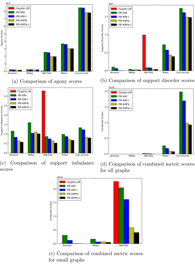
Figure 4.1: Metric scores of the algorithms on all real-life graphs for 10 levels. Gupte-LM could not finish its execution within the 24 hours time limit on Ama-zon, Webg, Pokec and Live Journal graphs. Therefore, its results on those graphs are not shown in the charts. Overall, we observe similar metrics for the base-line solutions (Gupte-LM and PR-KM), while our methods reduce the combined
Table 4.1: Vertex and edge information of real-life graphs Short name # of nodes # of edges Description
Amazon 403,394 3,387,388 Amazon product
co-purchase history
Webg 875,713 5,105,039 Web graph
from Google WikiTalk 2,394,385 5,021,410 Wikipedia talk
(communication) network Pokec 1,632,803 30,622,564 Pokec online
social network Live Journal 4,847,571 68,993,773 LiveJournal online
social network Table 4.2: Vertex and edge information of synthetic graphs
Name RMAT scale # of nodes # of edges
rmat0 20 65,536 1,044,911 rmat1 21 131,072 2,091,937 rmat2 22 262,144 4,186,472 rmat3 23 524,288 8,377,152 rmat4 24 1,048,576 16,760,098
4.1
Experiment Setup
We used five real-life graphs and five randomly generated synthetic graphs in our experiments. The real-life graphs were taken from Stanford Network Analysis Project (SNAP) [7]. The list of the graphs that we took from the SNAP library along with their vertex and edge properties are listed in Table 4.1.
We generated our synthetic graphs using the R-MAT generator of the Boost library [8]. The R-MAT generator creates small world graphs for given sizes. However, the R-MAT generator may create self loops meaning a vertex can have and edge to itself. Therefore, we needed to remove those edges. Thus, we created graphs with 2scale edges and 2scale−4 vertices, then removed the self loops. In the end, we created the graphs described in Table 4.2.
of our algorithms on different types of social graphs. As we can see from their description, they originate from different use-cases. On the other hand, we also needed to investigate the impact of the graph size on the running time of our algorithms and the resulting values of the different metrics. Since all synthetic graphs are generated using the same tool, these graphs have similar network structure. In order to measure the impact of the number of levels on the metric scores, we tested our method on the real life graphs, partitioning them into 5, 10, 20, 40, and 80 levels.
We tested our methods on a server with 2 intel E5520 2.27 GHz processors and 48 GB of RAM. We decided the time limit for our experiments as 24 hours; therefore, algorithms that need more than 24 hours to execute are excluded from our charts.
4.2
Metric Results
We first compare and analyze the results of the algorithms in terms of agony, suppor disorder, support imbalance and the combined metric on the-real life graphs, which are shown in Figure 4.1.
4.2.1
Agony
We expected Gupte-LM solution to have low agony while the PR-KM solution to have high agony. Our experiments validated our expectections. Since our proposed methods are similar to PR-KM, we did not expect their solutions to differ greatly from those of PR-KM in terms of agony. However, PR-KM%-I reduced the combined metric by almost 15% compared to PR-KM.
(a) Running time comparison of all algo-rithms for 10 levels
(b) Running time of PR-KM%-I for num-ber of levels of 5, 10, 20, 40, and 80
(c) Running time of PR-KM%-I for differ-ent sized sythetic graphs described in Ta-ble 4.2 for 10 levels
Figure 4.2: Running times of the algorithms on real-life and synthetic graphs. Gupte-LM could not finish its execution within the 24 hours time limit on Ama-zon, Webg, Pokec, Live Journal graphs, and the biggest sythetic graph. Therefore, its running times on those graphs were not included.
4.2.2
Support Disorder & Support Imbalance
Since the primary concern of Gupte-LM is agony, our expectation was to see it perform worse on support related metrics compared to PR-KM, the other base-line algorithm. Also, we expected to see improved results for our algorithms on support related metrics as well. While the test results verified our presump-tions, PR-KM%-I reduced the support related metrics by almost 50% compared to PR-KM.
4.2.3
Combined Metric
Our baseline algorithms concentrates on seperate metrics. While Gupte-LM fo-cuses on minimizing agony, PR-KM fofo-cuses on minimizing support disorder and support imbalance scores. However, the test results show that their strengths and weaknesses cancel out, and they both produce similar combined metric scores.
Our algorithms out-perform the baseline algorithms in terms of the combined metric. Even though PR-KM%-I did not always have a very big advantage over PR-KM, switching to PR-KM%-I reduced the combined metric by at least 53% and on average 74% on the real-life graphs that we tested. Also, on the Amazon sales graph KM%-I reduced the combined metric by 98% compared to PR-KM.
4.3
Running Time
We ran the algorithms on the real-life graphs using different number of levels to investigate the effect of the number of levels on the running times. We also investigated the impact of the graph size on the running times of the algorithms, by running the algorithms on synthetic graphs of varying size. The results are shown in Figure 4.2.
(a) Agony (b) Support Disorder
(c) Support Imbalance (d) Combined
Figure 4.3: The effect of the number of levels on the metric scores of PR-KM%-I. The numbers of levels used in this experiment are 5, 10, 20, 40, and 80.
PR-KM is the best algorithm in terms of running time in our tests followed by PR-KM-I. PR-KM% produces a faster running time on WikiTalk graph, how-ever it is worse than PR-KM-I on other graphs. PR-KM%-I is unsurprisingly slower than both of the methods it used. On the other hand, our second baseline algorithm, Gupte-LM is the slowest method we tested. It could not finish its execution within the time limit on 50% of the graphs that we used for our tests. As we can see from Figure 4.2, it is asymptotically slower than any other method we tested.
4.4
Number of Levels
As discussed in §4.2 and §4.3, PR-KM%-I achieves the best combined metric in exchange for an acceptable level of increase in computational effort. In this section, we discuss the effect of the number of levels on the metric scores of PR-KM%-I. We ran the algorithm on the real-life graphs using 5, 10, 20, 40, and 80 levels. The results are shown in Figure 4.3.
The metric scores of PR-KM%-I followed similar patterns on all of the real-life graphs tested. Agony and support disorder increased as the number of levels increased as expected, because more of the low support nodes with high level connections were seperated from high levels as the number of levels increased. Similarly, more of the nodes with high support having many low level connec-tions were kept at the lower levels. However, these nodes caused more support disorder as the number of levels increased. Conversely, support imbalance de-creased as the number of levels inde-creased, because the levels became less crowded and more marginal. Thus, the variance of support and support imbalance de-creased. However, lower support imbalance score could not bring the combined metric down and the combined metric increased as the number of levels increased.
4.5
Similarity of Algorithms
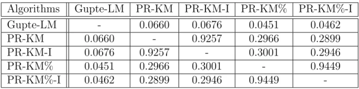
We used Normalized Mutual Information [9] to measure similarities between level assignments of algorithms we discuss. NMI takes values between 0 and 1; and high NMI score means high similarity for level assignments. NMI values for all algorithms for WikiTalk graph for 10 levels is shown at Table 4.3. Since, PR-KM-I is a iteratively improved version of PR-KM, their similarity score is high. Similarly, PR-KM% and PR-KM%-I are similar as well. However, difference be-tween PR-KM and PR-KM% is significantly more because majority of vertices were assigned one by one in PR-KM% approach; thus, using Partial Placement
Table 4.3: Normalized Mutual Information of Algorithms for WikiTalk Algorithms Gupte-LM PR-KM PR-KM-I PR-KM% PR-KM%-I
Gupte-LM - 0.0660 0.0676 0.0451 0.0462
PR-KM 0.0660 - 0.9257 0.2966 0.2899
PR-KM-I 0.0676 0.9257 - 0.3001 0.2946
PR-KM% 0.0451 0.2966 0.3001 - 0.9449
PR-KM%-I 0.0462 0.2899 0.2946 0.9449
-§ 3.3.2 is reducing similarity between level assignments noticeably. Lastly, Gupte-LM’s level assignment is very different compared to all other approaches, while PR-KM, PR-KM-I, PR-KM% and PR-KM%-I produced more similar level as-signments due to latter 3 being based on PR-KM approach.
4.6
Comparison of All Algorithms
In this section, we summarize the performance of all of the algorithms.
4.6.1
Gupte-LM
This baseline method aims at producing low agony score. Even though it has significantly better results on the agony metric, this algorithm performs very poorly on the support related metrics. As a result, it produces worse combined metric scores. On the other hand, the biggest problem with this method is its slow running time. In Gupte et al. [1], finding the biggest Eulerian cycle within the graph is done by the repetitive process of finding a cycle and adding them together. Unfortunately, this process takes a significant amount of time. Thus, this method did not complete its execution within the 24 hour time limit for four of the five natural graphs we used in our tests.
4.6.2
PR-KM
Our second baseline aims at achieving low support metric scores. It forms the basis of our proposed algorithms. Thus, it was the main benchmark for the performance of our algorithms in terms of the combined metric score. It has the lowest running time requirement among the five methods as well.
4.6.3
PR-KM%
KM solution focuses solely on the support metrics. We have developed PR-KM% by incorporating the partical placement approach into PR-KM, in order to achieve better results in terms of agony. Even though PR-KM% was slower than PR-KM-I in most of our tests, it always had a better combined metric score than PR-KM-I. Thus, PR-KM% lead to the best combined metric score values.
4.6.4
PR-KM-I
PR-KM-I tries to improve a solution given by PR-KM by making incremental changes. It lead to approximately 20% improvement in our tests, which is a big plus considering it could be used on any solution for the social hiearchy problem.
4.6.5
PR-KM%-I
PR-KM%-I combines our two proposed methods: partial placement and iterative improvement. It performs better than both of the baseline solutions. This is the second slowest algorithm that we tested. On the other hand, the difference in the execution time is not huge. Therefore, we deem it the most suitable approach to find social hierarchy in directed social networks for any given number of levels.
(a) Agony (b) Support Disorder
(c) Support Imbalance (d) Combined
Figure 4.4: Metric results for different graph sizes on synthetic graphs. Number of vertices and edges of graphs that are used in this experiment are shown in Table 4.2. Gupte-LM could not finish its execution in 24 hours time limit for one of the graphs; thus, it is not included in graphs. Number of levels in this experiment is 10.
Chapter 5
Related Work
After our literature search for finding hierarchy in social graphs, we classified papers we found into 3 categories. Some of them were focusing on a metric similar support to find hierarchy in directed networks. Some other papers were using agony to find hierarchy within networks. Also, there were some other works which used different approaches to find hierarchy within social networks.
PageRank algorithm [2] was the first algorithm that comes to mind when trying to find most popular and less popular vertices in directed graphs. Our support metric is basically popularity of vertex within graph; therefore, PageRank was one of the algorithms that captures support aspect of our project. This algorithm basically gives all nodes a PageRank score based on their connections within network and a vertex’s popularity calculated from its incoming edges. Brink et al. [10] focuses on β-measure and score-measure to find hierarchy within directed networks. β-measure basically counts the number of incoming edges for each vertex, then each vertex gains β-measure score from its outgoing vertices inversely proportional to those vertices’ number of incoming edges. Rowe et al. [11] looks at coonnections between vertices and graph’s structure. He uses number of edges between nodes, mean of shortest path from a specific vertex to other vertices in graph, number of cliques, betweenness centrality and similar metrics to find a ranking score for each vertex. Then, he assigns each vertex to a
level based on its score. Also, Elo [12] and Glicko 1&2 [13] algorithms are ranking systems for players based on matches between them.
Gupte et al. [1] is one of the many papers focusing on agony to partititon a graph. It first finds the biggest Eulerian within the graph. After that step, remaining graph will be reduced to a directed acyclic graph and a cycle. Then Gupte et al. assigns each node to a level minimizing number of levels and he also proves his method creates one of the perfect level assignments. Tatti et al. [14] proposed an algorithm for faster calculation for a level assignment mini-mizing agony* (I think it doesn’t find maximum Eulerian). However, it doesn’t find the maximum eulerian in some cases. Thus, we avoided it. On different paper, Tatti et al. [15] gives an algorithm for finding minimum agony partition on directed graphs with different edge weights. He reduces that problem to ca-pacitated circulation problem, a polynomial solution. Minimum feedback arc set problem is another similar algorithm, which is proven to be NP-Hard [16]. Few poly-logaritmic approximate solutions for this problem are already given [17].
Macchia et al. [18] proposed an algorithm that finds a summary for a directed graph by merging DAGs which are homogenous and have low total agony. Mac-chia measures homogenousity of a DAG with Jaccard coefficient. Maiya and Berger-Wolf [19] assumed links between vertices are influenced by underlying hi-erarchy. Mones et al. [20] proposes to use Gloabal Reaching Centrality (GRC) to measure hierarchy in networks. Slikker et al. Focuses on finding hierarchy in Di-rected acyclic graphs [21]. Newman et al. [22] removes links to find communuties within network. Clauset et al. [23] tries to find hieararchy within graph without knowing all of the properties. Leskovec, Huttenlocher, and Kleinberg showed relatation within social network can be negative as well as positive [24] and pro-posed an algorithm to detect sign of a link [25]. Wang et al. [26] propro-posed an algorithm to find hierarchies within communication interaction networks (CIN) based on messaging information among its users. Klienberg et al. [27] gave an algorithm to find authoritative and reliable pages in hyperlinked environment.
Chapter 6
Conclusion
In this thesis, we developed a new metric to measure the quality of a given hierarchy in directed social networks. Traditional methods either used agony or support to measure quality of proposed hierarchy, instead we used both agony and support. Then, we developed an efficient algorithm that finds level assignment for the vertices in a directed social network and compared its performance with 2 baseline solutions, one focusing on agony the other focusing on support. We showed our proposed algorithm reduces objective score significanly on real-life and synthetic graphs. On top of that, our proposed algorithm includes and iterative improvement method in it; therefore, any other algorithm trying to find level assignment for lower objective score can benefit from it.
Bibliography
[1] M. Gupte, P. Shankar, J. Li, S. Muthukrishnan, and L. Iftode, “Finding hierarchy in directed online social networks,” in Proceedings of the 20th In-ternational Conference on World Wide Web, WWW ’11, pp. 557–566, New York, NY, USA: ACM, 2011.
[2] L. Page, S. Brin, R. Motwani, and T. Winograd, “The PageRank citation ranking: Bringing order to the web,” Tech. Rep. SIDL-WP-1999-0120, Stan-ford InfoLab, 1999.
[3] G. Karypis and V. Kumar, “Multilevel graph partitioning schemes,” in Proceedings of the International Conference on Parallel Processing (ICPP), pp. 113–122, 1995.
[4] T. H. Cormen, C. Stein, R. L. Rivest, and C. E. Leiserson, Introduction to Algorithms. McGraw-Hill Higher Education, 2nd ed., 2001.
[5] A. V. Goldberg and T. Radzik, “A heuristic improvement of the bellman-ford algorithm,” Applied Mathematics Letters, vol. 6, no. 3, pp. 3–6, 1993. [6] B. V. Cherkassky, A. V. Goldberg, and T. Radzik, “Shortest paths
algo-rithms: Theory and experimental evaluation,” Mathematical programming, vol. 73, no. 2, pp. 129–174, 1996.
[7] J. Leskovec and A. Krevl, “SNAP Datasets: Stanford large network dataset collection.” http://snap.stanford.edu/data, June 2014.
[8] J. G. Siek, L.-Q. Lee, and A. Lumsdaine, Boost Graph Library, The: User Guide and Reference Manual. Addison-Wesley, 2002.
[9] A. Strehl and J. Ghosh, “Cluster ensembles—a knowledge reuse framework for combining multiple partitions,” Journal of machine learning research, vol. 3, no. Dec, pp. 583–617, 2002.
[10] R. Van Den Brink and R. P. Gilles, “Measuring domination in directed net-works,” Social Networks, vol. 22, no. 2, pp. 141–157, 2000.
[11] R. Rowe, G. Creamer, S. Hershkop, and S. J. Stolfo, “Automated social hierarchy detection through email network analysis,” in Proceedings of the 9th WebKDD and 1st SNA-KDD 2007 workshop on Web mining and social network analysis, pp. 109–117, ACM, 2007.
[12] A. E. Elo, The rating of chessplayers, past and present. Arco Pub., 1978. [13] M. E. Glickman, “Parameter estimation in large dynamic paired comparison
experiments,” Applied Statistics, pp. 377–394, 1999.
[14] N. Tatti, “Faster way to agony,” in Machine Learning and Knowledge Dis-covery in Databases, pp. 163–178, Springer, 2014.
[15] N. Tatti, “Hierarchies in directed networks,” in Data Mining (ICDM), 2015 IEEE International Conference on, pp. 991–996, IEEE, 2015.
[16] V. Kann, On the approximability of NP-complete optimization problems. PhD thesis, Royal Institute of Technology Stockholm, 1992.
[17] G. Even, J. S. Naor, B. Schieber, and M. Sudan, “Approximating minimum feedback sets and multicuts in directed graphs,” Algorithmica, vol. 20, no. 2, pp. 151–174, 1998.
[18] L. Macchia, F. Bonchi, F. Gullo, and L. Chiarandini, “Mining summaries of propagations,” in Data Mining (ICDM), 2013 IEEE 13th International Conference on, pp. 498–507, IEEE, 2013.
[19] A. S. Maiya and T. Y. Berger-Wolf, “Inferring the maximum likelihood hier-archy in social networks,” in Computational Science and Engineering, 2009. CSE’09. International Conference on, vol. 4, pp. 245–250, IEEE, 2009.
[20] E. Mones, L. Vicsek, and T. Vicsek, “Hierarchy measure for complex net-works,” PloS one, vol. 7, no. 3, p. e33799, 2012.
[21] M. Slikker, R. P. Gilles, H. Norde, and S. Tijs, “Directed networks, allocation properties and hierarchy formation,” Mathematical Social Sciences, vol. 49, no. 1, pp. 55–80, 2005.
[22] M. E. Newman and M. Girvan, “Finding and evaluating community structure in networks,” Physical review E, vol. 69, no. 2, p. 026113, 2004.
[23] A. Clauset, “Finding local community structure in networks,” Physical re-view E, vol. 72, no. 2, p. 026132, 2005.
[24] J. Leskovec, D. Huttenlocher, and J. Kleinberg, “Signed networks in social media,” in Proceedings of the SIGCHI conference on human factors in com-puting systems, pp. 1361–1370, ACM, 2010.
[25] J. Leskovec, D. Huttenlocher, and J. Kleinberg, “Predicting positive and neg-ative links in online social networks,” in Proceedings of the 19th international conference on World wide web, pp. 641–650, ACM, 2010.
[26] Y. Wang, M. Iliofotou, M. Faloutsos, and B. Wu, “Analyzing communi-cation interaction networks (cins) in enterprises and inferring hierarchies,” Computer Networks, vol. 57, no. 10, pp. 2147–2158, 2013.
[27] J. M. Kleinberg, “Authoritative sources in a hyperlinked environment,” Jour-nal of the ACM (JACM), vol. 46, no. 5, pp. 604–632, 1999.