A POLICY FOR THE MAINTENANCE OF A
MULTISTATE MULTICOMPONENT SERIES
SYSTEM
ATHESIS
SUBM IHED TO THE DEPARTMENT OF INDUSTRIAL
ENGINEERING
AND THE INSTITUTE OF ENGINEERING AND SCIENCES
OF BILKENT UNIVERSITY
IN PARTIAL FULFILLMENT OF THE REQUIREMENTS
FOR THE DEGREE OF
MASTER OF SCIENCE
By
Alev Kaya
July, 1997
SYSTEM
A THESIS
SUBMITTED TO THE DEPARTMENT OF INDUSTRIAL ENGINEERING
AND THE INSTITUTE OF ENGINEERING AND SCIENCES OF BILKENT UNIVERSITY
IN PARTIAL FULFILLMENT OF THE REQUIREMENTS FOR THE DEGREE OF
MASTER OF SCIENCE
By
A lev KayaJuly, 1997
T S
•lí39 1 9 3T
I certify that I have read this thesis and that in my opinion it is fully adequate, in scope and in quality, as a thesis fot the degree of Master o f Science.
Assoc. Prof. Ülkü GürleırPrincrg^ Advisor)
I certify that I have read this thesis and that in my opinion it is fully adequate, in scope and in quality, as a thesis for the degree of Master of Science.
Assoc. Prof. Cemal Dinçer
I certify that I have read this thesis and that in my opinion it is fully adequate, in scope and in quality, as a thesis for the^^legrefe ^pf Master o f Science.
A . V
Assoc. Prdf.\ Yasemin Serin
Approved for the Institute o f Engineering and Sciences:
Prof. Mehmet Baray y .
ABSTRACT
A P O L IC Y F O R T H E M A IN T E N A N C E O F A M U L T IS T A T E M U L T IC O M P O N E N T SER IES S Y S T E M
A lev Kaya
M .S . in Industrial Engineering Supervisor: Assoc. Prof. Ülkü Gürler
July, 1997
In real life situations various levels of performance for both systems and components are identified. Deterioration of systems and components has been considered by many maintenance and replacement models in the literature, but most of these models are for single component. Our study concerns a multistate multicomponent maintenance model. We extended the model studied by Van der Duyn Schouten and Vanneste (1993) with four states, (0 ,1 ,2 ,3 ), to a multistate system with 5 +
1
states, (0
,1
, . . . , S). While classifying these S + 1states, we use two different classification schemes corresponding to different real life situations. Then, we analyze our model under both exponential and Erlang sojourn time distributions for both state classification schemes. As a result of our analysis, we derive expressions for the long-run average cost per unit time. We used the randomization method to evaluate the transient state probabilities during the implementation of the average cost expressions.
Key words: Maintenance Policies, Continuous-Time Markov Processes, Randomization Method.
Ç O K E V R E L I Ç O K B IL E ŞE N L I SER İ B İR S İS T E M İÇ İN B İR B A K IM K U R A L I
A lev Kaya
Endüstri Mühendisliği Bölümü Yüksek Lisans
Tez Yöneticisi: Doç. Ülkü Gürler
Tem m uz, 1997
Gerçek yaşamda hem sistemler hem de bileşenler için çeşitli performans düzeyleri belirlenebilir. Sistemlerin ve bileşenlerin yıpranması birçok bakım ve değiştirme modelinde dikkate alınmıştır. Ama bu çalışmaların çoğu tek bileşeni! sistemler içindir. Bu tez çalışması çok bileşenli ve çok evreli bir bakım modeli üzerinedir; Van der Duyn Schouten and Vanneste (1993) tarafından dört evreli olarak çalışılan bir model, çok evreli olarak genişletilmiştir. Evreler iki farklı şekilde sınıflandırılmış, ve model her iki sınıflandırma altında üssel ve Erlang kalış süresi dağılımları için analiz edilmiştir. Bu analiz sonucunda uzun dönemde birim zaman ortalama maliyeti veren ifadeler elde edilmiştir. Bu ifadelerde yer alan geçici durum olasılıklarının hesaplanmasında rassallaştırma metodu kullanılmıştır.
Anahtar sözcükler: Bakım Kuralları, Sürekli-Zaman Markov Süreçleri, Rassallaştırma.
I would like to express my gratitude to Assoc. Prof. Ülkü Gürler due to her supervision, suggestions, and understanding to bring this thesis to an end.
I am indebted to Assoc. Prof. Cemal Dinçer and Assoc. Prof. Yasemin Serin for showing keen interest to the subject matter and accepting to read and review this thesis.
I would like to thank Özgür Atilla, Barış Balcıoğlu, Murat Bayiz, Savaş Dayanık, Muhittin Demir, Nebahat Dönmez, Ali Erkan, Hülya Emir, Feryal Erhun, Fatma Gzara, Bahar Kara, Kemal Kılıç, Hakan Özaktaş, Serkan Özkan, Muzaffer Tanyer, Souheyl Touhami, and Faker Zouaoui for their moral support and help during the preparation of this thesis.
Contents
1 Introduction and Literature Review
1.1
Maintenance Policies1.2 Literature Review
2 Model Definition and Preliminaries 9
2.1
Description of the Main Model2.2 Possible Applications and M o tiv a tio n ...
1.3
2.3 Exact Method for
7
T;s and7
T(;j) S ... 142.4 Determining
7
T;s and7
T(/j) S ...1.5
2.5 Preliminaries for Analytical Results 19
3 Analytical Results 24
3.1 Analysis of the Model under First C lassification ... 24
3.1.1 Case
1
: Exponential Analysis 243.1.2 Case
2
; Erlang A n a ly s is ... 333.2
Aucilysis of the Model under Second Classification 363
.2.1
Case 3: Exponenticil A n a ly s is ... 363.2.2 Case 4: Erlang A n a ly s is ... 38
4 Implementation of the Model 42 4.1 Transient Solutions for Continuous-Time Markov Processes . . . 43
4.1.1 Randomization Method 45 4.2 Cost E valu ation... 46
4.3 Optimization M e th o d ... 49
4.4 Examples 49 4.4.1 Example
1
... 504.4.2 Example 2 ... 52
5 Conclusion 55 A Detailed Analytical Results 57 A .l Results Under First C lassification... 57
A.
1.1
Case1
: Exponential A n a ly s is ... 57A.
1.2
Case 2: Erlang A n a ly s is ... 59A
.2
Results Under Second Classification... 62A .
2.1
Case 3: Exponential A n a ly s is ... 62List of Figures
2.1
Case1
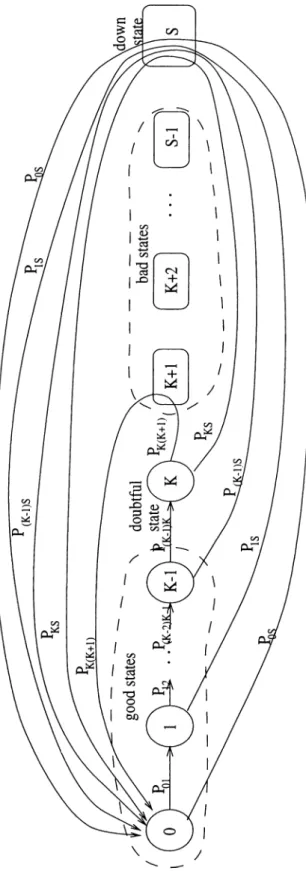
: Probability transition diagram of ,n,· > 0 } ... 162.2
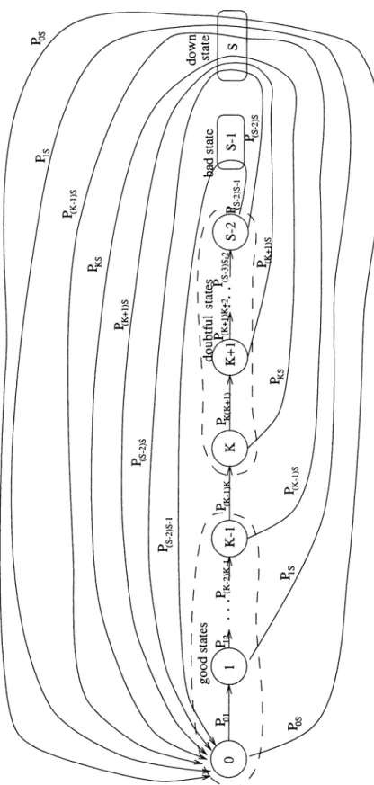
Case 3: Probability transition diagram of {X „, , ni >0
} ... 172.3 Representation of state I under the Cases
2
and 4 ... 182.4 Transition rate diagram of { F ( i ) , f >
0
} 192.5 Transition rate diagram of { Z ( i ) , f >
0
}21
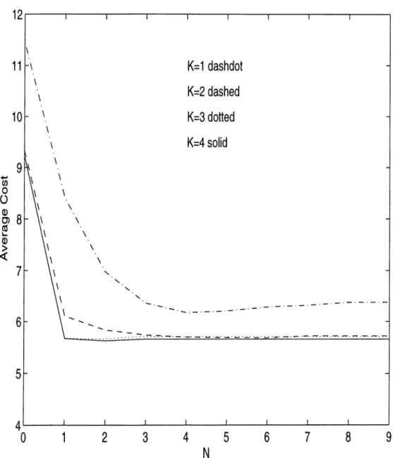
2.6 Transition rate diagram of { W{ t ) , t > 0 } ... 22 4.1 Example
1
: Cost curves for =1
,2
, 3, 4 through all possibleN 54
2.1 Ranges of / and j of
7
T;s and7
T(/j) S ... 14 4.1 Example1
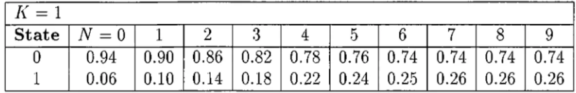
: For /i = 1, probability distributions for all possibleN 50
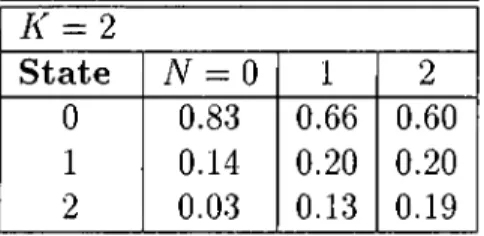
4.2 Example
1
: For K =2
, probability distributions for all possibleN 50
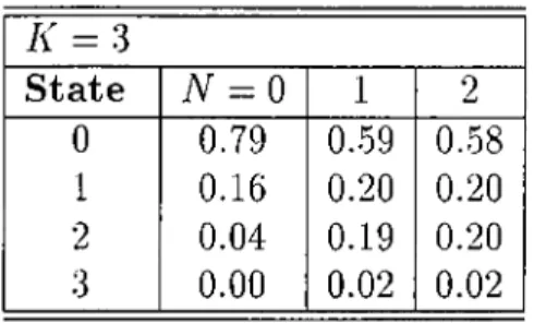
4.3 Example
1
; For K = 3, probability distributions for all possibleN 51
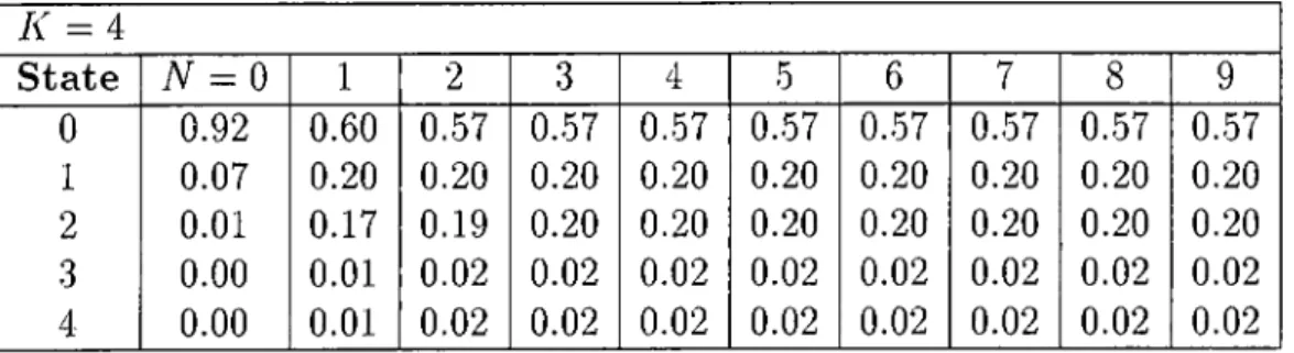
4.4 Example
1
: For K = 4, probability distributions for all possibleN 51
4.5 Example
1
: Average cost v a lu e s ... 514.6 Example
2
: For /i =1
, probability distributions for all possibleN 52
4.7 Example 2: For K = 2, probability distributions for all possible
N ... 52 4.8 Example
2
: For K = 3, probability distributions for all possibleN 53
4.9 Example
2
: For K =1
and =1
, comparison of our probability distribution with the exact distribution ... 53Chapter 1
Introduction and Literature
Review
In many real life situations the systems and their components are capable of assuming a whole range of levels of performance, varying from perfect functioning to complete failure. There is a growing interest in the maintenance and replacement of multistate systems indicated by the vast amount of existing literature. However, most of these studies consider single component systems. Multistate, multicomponent maintenance systems have become more popular since 1990’s, partly because of their applicability in the design and operation of computers and other service facilities as well as in the traditional areas like road maintenance, the aircraft industry, and oil production.
In maintenance optimization models the goal is to find the right compromise between preventive maintenance which extends the period of proper operation of the systems and corrective maintenance or replacement which replaces an old system by a new one. The decision process of when to replace the system becomes rather involved when the system is composed of many components that require maintenance. In these situations, an important issue is when to combine maintenance and replacement activities on several components.
1.1
Maintenance Policies
Before reviewing the literature on multistate maintenance and replacement models, let us review some of the mostly used policies [
8
].• Replacement upon failure. Consider a device operating continuously in time. Replacement upon failure requires that it is replaced by a new one at each time it fails.
• Block replacements. An item is replaced upon failure and at fixed times
D , 2 D , 3 D , ... where D > Q. Such a replacement policy is called block replacement. This policy is suitable if the system is composed of many items, all of which operate at the same time (such as a block of light bulbs in some public hall). Then, the whole block of items is replaced at the times D ,2 Z ),3 D ,.... In addition, if a single unit fails before the scheduled repair times then, it is replaced immediately.
• Age replacement. An item is replaced upon failure or when it reaches
the predetermined age D, where Z) is a fixed nonrandom age. Such
a replacement policy is called age replacement policy or control limit policy. Age replacement is more difficult to administer than the block replacement because of the need to continuously keep the age of the item. However, one would exjDect less number of replacements under this policy.
• Modified age replacement. Under the modified age replacement policy the unit is replaced preventively at the first period at which there is no demand and its operational age exceeds some control limit.
• Minimal repair. The item is repaired each time it fails and the repair period is negligible so that it can be practically ignored. The repair does not make the item as good as new but leaves it as good as it was just before it failed.
• Imperfect repair. In some applications minimal repair or any repair may not be possible or feasible at the times of the failures. For example, the
CHAPTER 1. INTRODUCTION AND LITERATURE REVIEW
cost of the minimal repair is a random variable C . It may be reasonable to perform a minimal repair only if C < cq where cq is some constant which may be, e.g., the price of a new item. Denote p = P {C > cq}. Then one would minimally repair the component only with probability
1
— p, and with probability p will scrap it or replace it with a new component.1.2
Literature Review
Equipment maintainability started to become popular in mid 1960’s. Barlow and Proschan (1965) [
2
] and McCall (1965) [14] report the first published works. Pierskalla and Voelker (1976) [18], Sherif and Smith (1981) [20], Valdez-Flores and Feldman (1989) [25] and Cho and Parlar (1990) [4] cover a wide variety of the maintenance literature in their survey papers.Valdez-Flores and Feldman (1989) focus on the work done on single component systems. They classify single component preventive maintenance models as: inspection models, minimal rejDair models, shock models, and other replacement models [25]. Cho and Parlar (1990) [4] survey the literature related to optimal maintenance and replacement models for multicomponent systems.
Single component multistate maintenance and replacement models are more common in the literature with respect to two-component and multicomponent models. First, we review the existing literature for single component systems.
Gottlieb (1981) considers a device subject to a series of shocks which arrive as a semi-Markov process and cause a damage and eventually a failure. The optimal policy is shown to be a control limit policy [
6
].Berg (1984) proposes a preventive replacement policy for a unit that is in demand only part of the time and is inactive otherwise. Berg uses a marginal cost analysis to find the optimal control limit that minimizes the limiting conditional probability that the unit is down when it is demanded. He then compares the optimal limiting conditional probability that the unit is down
when it is demanded for the modified age replacement policy and the age replacement policy [3].
Tijms and Van der Duyn Schouten (1984) deal with a deteriorating equipment whose actual degree of deterioration can be revealed by inspection only. An inspection can be succeeded by a revision depending on the system’s degree of deterioration. In the absence of inspections and revisions, the working condition of the system evolves according to a Markov chain whose changes of the states are not observable with the possible exception of a breakdown. A special-purpose Markov decision algorithm operating on the class of control- limit rules is developed for the computation of an average cost optimal schedule of inspections and revisions [24].
Wijnmalen and Hontelez (1990) [30] point out the shortcomings of the algorithm published by Tijms and Van der Duyn Schouten (1984) [24] and present appropriate improvements.
Ohnishi et al. (1986) investigate an optimal inspection and replacement problem for a discrete-time Markovian deterioration system. It is assumed that the system is monitored incompletely by a certain mechanism which gives the decision maker some information about the exact state of the system. The problem is to obtain an optimal inspection and replacement policy minimizing the expected total discounted cost over an infinite horizon and formulated as a partially observable Markov decision process. Furthermore, under some reasonable conditions reflecting the practical meaning of the deterioration, it is shown that there exists an optimal inspection and replacement policy in the class of monotonic-four region policies [15].
W ood (1988) develops a preventive maintenance model for a constantly monitored multistate system, such that the damage to the system accumulates
via a continuous time Markov process. It is shown that, under certain
conditions the optimal restoration policy for system is a control limit rule [31].
CHAPTER 1. INTRODUCTION AND LITERATURE REVIEW
Jayabalan and Chaudhuri (1992) study the imperfect preventive mainte nance and replacement schedule for a system which works below a specified failure rate. For a given planning period, the optimal schedule for replacements
to minimize the total cost is obtained. Also, a branching algorithm with
effective dominance rules to obtain the optimal schedule is presented [
11
].Ozekici and Günlük (1992) consider a device that deteriorates over time according to a Markov process so that the failure rate at each state is constant. The reliability of the device is characterized by a Markov renewal equation, and an increasing failure rate on average property of the lifetime is obtained. The optimal replacement and repair problems are analyzed under various cost structures. Furthermore, intuitive and counterintuitive characterizations of the optimal policies and results on some interesting problems are considered [17].
Sim and Endrenyi (1993) propose a Markov model for a continuously
operating device whose condition deteriorates with time in service. The
model incorporates deterioration and Poisson failures, minimal repair, periodic minimal maintenance, and major maintenance after a given number of minimal
maintenances. An exact recursive algorithm computes the steady-state
probabilities of the device. A cost function is defined using different cost rates for the different tyj^es of outages. Based on minimal unavailability or minimal costs, optimal solutions of the model are derived. Major maintenance is found seldom beneficial if optimal maintenance intervals are used. If a maintenance policy is based on non-optimal intervals between maintenances, periodic major maintenance can reduce costs in some cases [
22
].Dagpunar (1994) considers an age replacement strategy where down times are nonzero. He derives necessary and sufficient conditions for age replacement to be preferred to replacement on failure in terms of the minimum of the mean residual life function. When age replacement is indicated, he derives sufficient conditions for the existence of a global minimum to the asymptotic expected cost rate function [5].
Lam and Yeh (1994) consider state-age-dependent replacement policies for a multistate deteriorating system. The optimization criterion is to minimize
the expected long-run cost rate. A policy improvement algorithm to derive the optimal policy is presented. It is shown that under reasonable assumptions the optimal policies have monotonie properties [13].
Van der Duyn Schouten and Vanneste (1995) consider a preventive maintenance policy, which is based not only on the information about the age of the installation but also on the content of the subsequent buffer. For this integrated maintenance-production problem, a class of control limit policies which are nearly optimal and easy to implemented are analyzed. The analysis is based on the embedding technique from Markov decision theory. Also, a characterization of the overall optimal policy and comparisons of the best control limit policy with the overall optimal policy are provided [28].
We will now present a review of some of the studies considering multicom ponent systems (with more than two components).
Ozekici (1988) provides a characterization of the structure of the optimal policy for multicomponent systems with dependent lifetimes. The ages of the components are assumed to develop over time as an increasing Hunt process. Under fairly general assumptions, Ozekici shows that for the optimal replacement policy, the regions of the state space are connected subsets of the state space with certain regularity conditions for the boundaries [16].
Hsu (1991) formulates the preventive maintenance problem for serial stochastically deteriorating production systems as a mathematical model. Nu merical examples are used to provide managerial implications for maintaining
such systems. The results show that the operating characteristics of the
stations are interrelated; therefore it is important to examine the joint effects of a maintenance policy on the various stations of the production system simultaneously rather than study each station separately [9].
Van der Duyn Schouten and Vanneste (1993) consider optimal group maintenance policies for a set of identical machines subject to stochastic
failures. The control of the system is not based on the complete age
only. The compromise between these two extreme cases is established by introducing four possible states for each component: good, doubtful, preventive maintenance is due, and failed. Starting from a general model with general but identical lifetime distributions for the individual components, an approximate model is introduced such that the four possible states are identified with certain age intervals for each individual component. The sojourn times in the good
and the doubtful state are supposed to be exponentially distributed. For
this resulting approximate model, explicit exiDressions are derived for various performance measures. These results are used in presenting approximations for the performance measures of the original model [27].
In another related study, Jansen and Van der Duyn Schouten (1995) analyze the optimal preventive maintenance schedule for a production system consisting of a set of identical parallel production units. The lifetimes of the units are distributed with an increasing failure rate and are supposed to be statistically
independent. They first show that, in the case geometrically distributed
lifetimes and unit repair times, the optimal preventive maintenance policy is characterized by a single control limit. For the exponentially distributed lifetimes and repair times, and when the repair capacity is limited, it is shown that the optimal policy has a week monotonicity property, such that the number of units which remain in the operation increases with the number of available units. However, it is not necessarily true that, under the optimal policy, the number of units in standby position increases with the number of available units. Also, the case of non-exponential lifetime distributions are considered by assuming the lifetimes are composed of two non-identical exponential phases. A unit in its first life phase is called good, while a unit in its second phase is called doubtful [
10
].Van der Duyn Schouten and Vanneste (1990) [26] and Van der Duyn Schouten and Wartenhorst (1994) [29] study on multistate maintenance and replacement systems with two components.
CHAPTER 1. INTRODUCTION AND LITERATURE REVIEW 7
The class of maintenance policies described above take advantage of the information about the state (age) of every individual system component. On
the other hand, several authors such as, Assaf and Shantikumar (1987) [
1
] and Ritchken and Wilson (1990) [19] studied coordinated group maintenance policies which are based on the number of failed components in the system.Chapter 2
Model Definition and
Preliminaries
We will analyze a multistate multicomponent maintenance model controlled by a simple decision rule. However, this decision rule depends on both the age configuration of components and the number of failed components. As will be discussed below, our main model is an extension of the model developed by Van der Duyn Schouten and Vanneste (1993) [27].
2.1
Description of the Main Model
Now, we will state the assumptions concerning the main model that we study.
1) The system that we consider is composed of M identical and indepen dently operating components.
2) The components are connected in series.
3) The condition of each component is characterized by S + 1 possible states which correspond to certain age intervals.
0
is the best state and S is the down state. States are classified into four groups as good, doubtful, bad,and down. Details of two different state classifications which are used by the model are explained after the assumptions of the model.
4) From state /, which is a good or a doubtful stcite, a transition occurs to either state / + 1 or state S (down), with probabilities Pi(i+i) and
Pis = 1 — Pi{i+i)i respectively. Therefore, a component either gets one state older, or fails down.
5) Upon the entrance to one of the bad states, an immediate preventive maintenance, upon the entrance to the down state an immediate
corrective maintenance is carried out on that particular component. Both maintenance actions bring the component back into state
0
.6
) For preventive and corrective component replacements costs of ci and C2
are incurred respectively. System replacement cost is C
3
. We assume that, corrective replacement is more costly than the preventive replacement, i.e. C'2
> Cl. We also assume that, replacing the system costs less than replacing each component preventively or correctively, i.e. C3
< Mci.7) Both of the maintenance operations are instantaneous and the operation of the system is not interrupted.
8
) The sojourn times are distributed with parameters depending on theactual state. The distribution functions are assumed to be known. Note that sojourns in bad and down states are instantaneous because of the immediate preventive and corrective maintenance actions.
9) An economic dependency between the components arises by the control policy that is used.
We will analyze this model under two different state classifications which are stated below:
• First classification:
CHAPTER 2. MODEL DEFINITION AND PRELIMINARIES
11
ii) state K is classified as doubtful,
iii) states K + 1 to 5 — 1 are classified as preventive maintenance due (bad),
iv) state S is classified as down. • Second classification:
i) states
0
to K —1
are classified as good, ii) states K to S — 2 are classified as doubtful,iii) state S —
1
is classified as preventive maintenance due (bad), iv) state S is classified as down.Under each state classification we will analyze two cases where the sojourn time at state / is distributed as:
• Exponential with the probability density function
/,(t ) = v ie-’'·· • /j;-Erlang with the probability density function
flit) = - 1)!
where ki denotes the number of exponential stages. Therefore, we have four different cases to analyze.
Case 1. States of the components are classified according to first
classification and sojourn time at state / is exponential.
Case 2. States of the components are classified according to first
classification and sojourn time at state I is /:;-Erlang.
Case 3. States of the components are classified according to second
classification and sojourn time at state I is exponential.
Case 4. States of the components are classified according to second
Control Policy A complete system replacement is carried out when a single component enters a bad or a down state and the number of doubtful components at that moment is greater than or equal to a critical value, say N.
In order to implement the control policy described above we need two decision variables, K and N. First one is the variable according to which the classification of states is done, and the second one is the threshold value associated with the number of doubtful components.
The two state classifications given before apply to different situations. If the model uses the first classification, then bad states are determined by the model via determination of the variable K. On the other hand, the use of the second classification requires to define the bad states at the beginning. Therefore, in the cases where bad states are known a priori, the second classification should be used. For example, when human life is under consideration, we cannot take any risk. So, we need to know the bad states a priori.
The control policy described above requires detailed information about the state of every single component. If a single component enters a bad or a down state when the number of doubtful components equals N, it is important to know whether that component came from a good state or a doubtful state. In the first case this situation will give rise to a system replacement, in the latter case it will not.
In this study we investigate a group replacement policy which recognizes both the advantages and the disadvantages of individual component informa tion. On the one hand, it is obvious that detailed information about the state of each individual component is useful in determining an optimal group replacement policy. On the other hand, one has to admit that this detailed information is not always available and, if available gives rise to optimal policies which are hard to imj^lement.
Aim Our aim is to derive explicit expressions for the average number of system replacements per unit time as well as the expected number of preventive and corrective component replacements during a system’s lifetime. With the
CHAPTER 2. MODEL DEEINITION AND PRELIMINARIES
13
cost components, these expressions provide us with a tool for determining K
and N via the minimization of the long-run average cost of the system. We note that system replacement in our model is interpreted as replacement of all components.
2.2
Possible Applications and Motivation
Our model was inspired by the model developed by Van der Duyn Schouten and Vanneste (1993) [27]. In their model there are only four states: good, doubtful, bad, and down. Van der Duyn Schouten and Vanneste (1993) indicate that their model was inspired by the maintenance of a regioiicil railroad track [27]. Depending on the waives occurring in the rails, a certain segment of a section is classified in one of the three possible states: bad, doubtful, and good. Due to safety regulations a bad segment of a section has to be maintained without delay. Maintenance requires a specific piece of equipment, which lifts the rails, shakes the stones, and puts the rails back in their place. This machine is able to handle several hundreds of yards during one night. The transportation costs of the equipment are high and so are the hiring costs. So a regional manager may consider hiring the equipment not only for a single night, but for a longer period of time in order to maintain not a single segment but a complete section. In this way, the manager is able to save future transportation costs and can negotiate discounts. Similar types of decision problems occur in maintaining asphalted highways (cracking, textural damage), drain systems (leakage), and dam walls (rust).
Other possible applications on this model are the replacement of the tires of trucks for extraordinary transport (the states correspond to the profile regions of a tire), and the replacement of personal computers within a department (states of a PC correspond to either age or frequency of complaints).
Why do we extend the model studied by Van der Duyn Schouten and
Case Notation TTi TTi Range
0
< / < A' 0 < 1 < K0
< i < ki0
< / < ,5' -2
0
< / < . ? -2
0
< i < A;,Table
2
.1
; Ranges of / and j of7
T;s andsystem are represented by four states: good, doubtful, bad, and down.
However, availability of precise measurement devices enables us to obtain detailed information about the performance of systems and components. By introducing multistate maintenance systems we can evaluate this detailed information. Having just four states can be enough to represent the different performance levels of railroad tracks, but for more complex systems this may not be the case. Our model allows to have as much of states as required by the nature of the system.
In our analytical results we need the probability of a component to be at a particular deterioration state (under exponential sojourn times), or a stage (under Erlang sojourn times) under the given control policy. We will define
7
T/ and7
T(;j) as the probability of a component to be at state I and at the jth stage of state /, respectively, under the given control policy. For the ranges ofI and j of
7
T;s and please refer to Table2
.1
.2.3
Exact Method for
tt/sand
7T(/Let us define a stochastic process { A{ t ) , t > 0} = {{Ai{t), A2i t ) , . . . , AM{t))}
that represepts the state of each component at time t under the given control policy. Then, {A( t) N >
0
} is a continuous-time Markov process since ineach state entered exponential time is spent (minimum of M exponential
CHAPTER 2. MODEL DEEINITION AND PRELIMINARIES
15
Markov chain can be obtained via the use of transition probabilities given in assumption 4). The number of states of {A{ t) , t > 0} can be determined through the evaluation of ( K +
1
) ^ for Case1
, and (S —1
)^^ for Case 3. Therefore, for Case1
, if M = 5 and K = 4, then the number of states in the corresponding Markov chain is 5'^ = 3,125. In the same example, if M = 10, then the number of states for Case1
is 5^° = 9,765,625. Since it is not easy to determine tt/s and through this approach, we will use a different approach for this purpose. Before going into details of our model, we will give some preliminary results.2.4 Determining
tt/sand
In this section we will consider that the system operates under the natural policy, that is, the effect of the given control policy is disregarded.
Let us define a stochastic process {Xi{ t), t > 0}, which represents the state of component i at time t, i =
1
, . . . , M , for Cases1
and 3. >0
},i —
1
, . . . , M, has the following properties:1) Each time the process enters state /, amount of time it spends in / is exponential with mean 1/vi (departure rate is t>;).
2
) When it leaves /, it enters m with probability pim wherepii = 0 V/ Pirn= 1 V/.
l^m
Then, { Xi { t) , t > 0 }, i = 1 , . . . , M , is a continuous-time Markov chain. We can also define an embedded Markov chain of {Xi{t)N > 0 }, > 0 }, where
Xm denotes the ?
2
,th state visited. The transition diagrams of {Xn-,ni > 0} for the Cases1
and 3 with the state spaces {0
,1
, . . . , A' } and {0
,1
, . . . , 5 —2
} are given in Figures2.1
and2.2
respectively. Since, Erlang distribution canCHAPTER 2. MODEL DEFINITION AND PRELIMINARIES
17
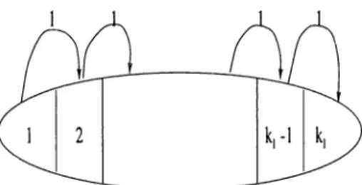
Figure 2.3; Representation of state I under the Cases
2
and 4be considered as a series of exponential distributions, we can represent state I
under the Cases
2
and 4 as a compound of ki exponential stages. Therefore, probability transition diagrams for the Cases2
and 4 can be obtained by considering each good and doubtful state in Figures2.1
and2
.2
, respectively, as the compound state illustrated in Figure 2.3.Remark 1 Under the Cases 2 and 4 a transition into a state can only be made
into the first stage, and out of a state can only be made from the last stage.
If we let our system work without any interruptions, that is, operate under the natural policy, tt/s and can be considered as the steady state probabilities
of {Xi( t)N > 0}. But, under the effect of the control policy, steady state may not be achieved before the system replacement. Therefore, tt/s and
7
T(/j)S cannot be the steady state probabilities.Remark 2 If we recall the control policy, we can expect the system to reach steady state before the system replacement when N is close to M and M is Icirge. But, this is not the case for N which is considerably smaller than M.
In Chapter 4, we will describe how we approximate tt/s and
7
rpj)S by using theCHAPTER 2. MODEL DEFINITION AND PRELIMINARIES
19
«0
a,
«2
0
^ (Xm OCmA ^ \ / )
0 ) i n f 2 ] · · · i i ^ ■·· (N-1)
1^1
^2
1^3
F'igure 2.4: Transition rate diagram of {Y{t), i > 0}
2.5
Preliminaries for Analytical Results
In our model, we will employ results from a continuous time birth-and-death
process. We will define a process t > 0} which represents the number
of doubtful components in the system under the given control policy. At each state, { Y{ t ) , t > 0} spends an exponential time. This is because the number of doubtful components changes when a component leaves its current state after spending an exponential time. Sum of exponential random variables results in an other exponential random variable. So, { Y{ t ) , t > 0} is a continuous-time Markov chain on { 0 ,
1
, . . . , A } governed by the transition diagram given in Figure 2.4. Here, node A represents the situation in which the system replacement is triggered. In Figure 2.4,• Aj·, 0 < i < N — refers to rate of transitions from node i to node ¿ +
1
, • Xn refers to rate of transitions from node N to node A ,• ^ ^ i ^ N, refers to rate of transitions from node i to node i —
1
, and • Qi, 0 < i < N, refers to rate of transitions from node i to itself.We need to make the following definitions:
• A backward jump of { Y{ t ) , t > 0} is a transition from some node i to ¿ -
1
.• A dummy jump of { Y{ t ) N >
0
} is a transition from some node i to itself. Therefore,• Backward jumps correspond to transitions of a single component from the doubtful state via an instantaneous bad or down state to a good state.
• Dummy jumps corresj^ond to transitions of a single component from a good state via an instantaneous down state back to a good state.
We should note that, backward jumps are associated with either preventive or corrective replacements, while dummy jumps are always associated with corrective replacements.
In order to obtain the average number of system replacements per unit time as well as the expected number of preventive and corrective component replacements during a system’s lifetime, we need the following quantities:
T j - == the expected entrance time of { T ( i ) , i > 0} into node A , given that F (0) = 0 < i < N;
Ki,N = the expected number of backward jumps of {Y'{t)N > 0}
before entrance into node A , given that F (0) = 0 < i < N] = the expected number of dummy jumps of { Y{ t ) , t > 0} before
entrance into node A , given that T (0) = 0 < i < N.
Explicit expressions for the quantities Ki,Ni Ti,N are given in the
following theorem proposed by Karlin and Taylor (1975)[12].
Theorem 1 (Karlin and Taylor)
- X ] T---- X Oiipi, Q < i < N
j = i l=zO
K..H =
CHAPTER 2. MODEL DEFINITION AND PRELIMINARIES
21
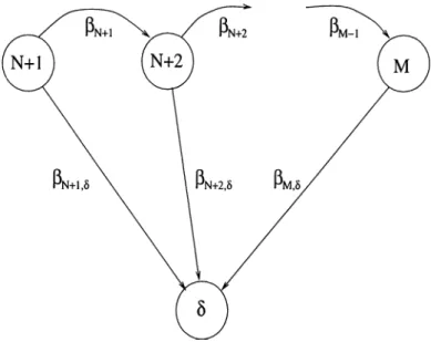
Figure 2.5: Transition rate diagram of {Z{t)N > 0}
N 1 i T-.N = — Ylph 0 < i < A f , j-i ^iPj 1=0 where po = Aq ^, pi = ^ and A
1
A2
. . . Xi-l c ^ ^ AT Pi —---, 2 < z < N. P1 P2 ■■■PiSimilar to {Y{t)N ^ 0 }, we consider the continuous-time birth-and-death
process { Z ( t ) , t > 0} which is defined on + with a transition
diagram as shown in Figure 2.5. Here {Z{t ),t > 0} again denotes the number of doubtful components and S repr esents a system replacement. In Figure 2.5,
• ^¿, N + l < i < M — I, represents the rtite of transitions from node i to node i + 1,
• (lis, N -{-1 < i < M, represents the rate of transitions from node i to node 6.
a„ a, «2 a. ttK
ai = the expected entrance time of {Z{t ),t > 0} into node given that Z(0) = N - \ - l < i < M.
Explicit expression for the quantity ai is obtained in the following theorem proposed by Karlin and Taylor (1975)[12].
Theorem 2 (Karlin and Taylor)
M
= E
1 Si
- i n +
i=i / ^ i + l=i
For the main model described above, let W{t) denote the number of doubtful
components at time i > 0. Similar to > 0} and {Z{t)N >
0 }, > 0} is a continuous-time Markov chain which is defined on
{ 0 , . . . , M ; The transition diagram for { W { t ) , t > 0} can be seen in Figure 2.6. It can be easily observed that Figure 2.6 can be decomposed into Figure 2.4 and Figure 2.5. As long as the number of doubtful components has not reached the level N + I and no system replacement is carried out,
> 0} behaves like {Y(t)N > 0} with a transition diagram as depicted in Figure 2.4. Moreover, from the moment at which the number of doubtful
CHAPTER 2. MODEL DEEINITION AND PRELIMINARIES
23
components is 1, until system replacement, the behcwior of { W { t ) , t > 0} is similar to that of {Z{t)N > 0} with a transition diagram as given in Figure 2.5. We also note that Xn in Figure 2.4 refers to sum of ¡In and /In,s in Figure 2.6. In addition to that, we consider node A in Figure 2.4 as a compound node of node N -\- 1 and node delta in Figure 2.6.
Analytical Results
In this chapter we will analyze the model under the four cases which were defined previously. As a result of this analysis we will obtain expressions for the average cost per unit time.
3.1
Analysis of the Model under First Clas
sification
In this section we will focus on the model when states are classified according to the first classification for both exponential and Erlang sojourn times in good and doubtful states.
3.1.1
Case 1: Exponential Analysis
Now, we will analyze Case 1. First, we will derive expressions for rates which are indicated in Figures 2.4 and 2.5. Then, we will use these expressions to obtain the expected time until system replacement, expected numbers
of preventive and corrective maintenance by using Theorems 1 and 2,
respectively. After that, we will derive an expression for the average cost per
CHAPTER 3. ANALYTICAL RESULTS
25
unit time. Before going ahead with the derivations, let us make some remarks.
Remark 3 Note that, the rates introduced in Figures 2.4 and 2.5 can be
interpreted as follows.
(a) Xi the rate of transitions due to which the number of
doubtful components increases, given that there are i
doubtful components, 0 < i — 1.
(b) Xn the sum of the rates of transitions due to which the
number of doubtful components increases and a system replacement is triggered, given that there are N doubtful components.
(c) ai the rate of transitions due to which the number of
doubtful components remains constant, given that there are i doubtful components, 0 < i < N.
(d) f.ti the rate of transitions due to which the number of
doubtful components decreases, given that there are i
doubtful components, 0 < i < N.
(e) I3i the rate of transitions due to which the number of
doubtful components increases, given that there are i
doubtful components, N - \ - \ < i < M — \.
(f) ¡3is the rate of transitions due to which a system repla
cement is triggered, N - \ - \ < i < M —
Remark 4 The number of doubtful components increases only when a
component at state K — 1 makes a transition into state K. We can observe it from Figure 2.1. Therefore, the increase in the number of doubtful components depends on the following:
1) expected number of components at state — 1, given
that there are i components at state A^,
2) deterioration rate of a component at state A' — 1, 3) probability that a component makes a transition from
Remark 5 A system replacement is triggered when one of the components at states 0 through K — 1 fails or enters a bad state, given that there are at least
N doubtful components. When there are N doubtful components, a system
replacement depends on the following:
1) expected number of components at states 0 through K — 1, given that there are N components at state
2) deterioration rates of components at states 0 through K — 1, 3) probabilities those components make transitions from states
0 through K — 1 to
When there are more than N doubtful components, then system replace
ment depends additionally on the following:
1) number of doubtful components at state K,
2) deterioration rate of a component at state K.
Remark 6 The number of doubtful components decreases when a component
at state K makes a transition into state K + 1 or state S. In both cases, the deteriorated component will be at state 0 after the instentanous preventive or corrective maintenance action. We can observe it from Figure 2.1. Since
Pk(k+i) and Pks adds up to unity, the decrease in the number of components depends on the following:
1) number of doubtful components at state /F, 2) deterioration rate of a component at state K.
Remark 7 Given there are less than N doubtful components, the number
of doubtful components remains constant due to instantaneous corrective maintenance actions followed by failures from good states.
1) expected number of components at states 0 through K — 1, given that there are i components at state K,
2) deterioration rate of a component at states 0 through — 1, 3) probabilities those components make transitions from states
CHAPTER 3. ANALYTICAL RESULTS
27
Remark 8 If we recall the control policy, a complete system replacement is triggered when a component enters one of the bad or the down states and the number of doubtful components at that time is greater than or equal to N.
So, if a good component fails down when the number of doubtful components is N, it cannot return back to the good state since a system replacement is triggered.
Remark 9 Let qij be defined by
qij — V i ^ ji,
i/i is the rate at which the process leaves state i and Pij is the probability that it then goes to j. It follows that qij is the transition rate from i to j.
Let us denote by Pij the probability that a Markov chain, presently in state i, will be in state j after an additional time t. That is.
It is known that
Pij = P { X { t + s ) = j \ X { s ) = г}.
,· Pijii) ■ / ·
t-^Q t
This can be observed from the following lines
P a W
lim
i—0 t limi-*0
lim t-*o Pij P { X i t ) ^ j \ X i O ) = i } t V it Pij + o(t) =
qij-Now, we are ready to propose the following results for transition rates indicated in Figures 2.4 and 2.5. Plea.se recall the notation introduced in Section 2.1, and in Figures 2.4 and 2.5.
Lemma 1 (a) (b) For 0 < i < N — I At· = ■^ A--lP(A--l)A-Oii
(c) A/v = {Yz;^(EzLo^7rzv;p,s + TT/V-VU/V-i) (c?) a;v = 0 jFor 0 < i < N (e) ( / ) (i/) Hi = Wa' F or A^ + 1 < i < M — I F or + 1 < i < M l^iS = T^l'^lPls) + iVK. Proof. Let Ff-l·] = conditional exj^ectation, F(·|·) = conditional probability,
n; = number of components at state /, 0 < / < K.
While making the proofs, we used the same method for all parts of Lemma 1. Therefore, here we will only prove part (c) of Lemma 1. For the other parts the reader is deferred to Section A. 1.1 in appendix for completeness.
As given in Remark 9, transition rates are determined simply as the product of a rate and a transition probability. But in our derivations we cannot write it so simply because the process for which we are determining the transition rates can make a transition depending on many other transitions made by the
M components which can be in various deterioration states. In addition to that, the process for which we are determining the transition rates does not tell the distribution of these M components among the deterioration states. We determine the transition rates of the process as the sum of the rates of
transitions made by those M component which result in the required transition
CHAPTER 3. ANALYTICAL RESULTS
29
do not know the distribution of the components we need to introduce expected values.
Therefore, please take into consideration the discussion we made above while reading the derivation below and the similar ones that you will encounter throughout the text.
Under consideration of Remarks 3b, 4, and 5 we have the following derivations for part(c) of Lemma 1.
K - 2
Aw = E[ni\riK = N]vipis + E[nK-i\nK = A^juw-i
1= 0 K - 2 M - N /=0 i(=0 M - N + X^ P{nK-i = jK-l\nK = N)jK-iVK-i i/s.'-l=0 K - 2 M - N ( M 7T; -1=0 ji=0 \nJ^k\^ ^h) . {N,jK-uM-N-jK_i)'^K^K-l(^ ^A'-l ^k) ^ ^ j K - i = 0 { T ) ^ K i ^ - f - N X jK-lVK-1 K - 2 M - N - jt,
-= E E
;=o ji=0 (1 - 7Ta-)^ -^ ' JfOlPtS . X ('1 _ ^ \ M - N J K - 1 V K - 1 jK-i=0 c ^K) \ M - N - j { - l I ^ M ^ - 1 (M - N )k i{ ^ II - 7T; - TTA')^ “ X X n _ TTr-i^-^ j ; = 0 c ^ h ) M ^ - i (M - N) n K- i - ^K-i - ^k) J'k-i=0 VK-\ -VlPlS (1 _ ^J.)M-N X —--- - ( > 7T/U;p/s + 7rw_iUA-_ij. (1 - ^ A ') S□
Observation 1 We can infer from Lemma 1 and its proof that, given there are i components at the doubtful state, other components are expected to be distributed among good states proportional with their j^robabilities to be found at those states.
Observation 2 As we mentioned earlier our model is a generalization of the model offered by Van der Duyn Schouten and Vanneste (1993) [27]. When state 1 is set as the doubtful one, the results presented in Lemma 1 reduces to the results given by Van der Duyn Schouten and Vanneste (1993) [27]. For
K = 1, Lemma 1 takes the following form;
Ai = {M -Av = [M -ßi = ivi, 0 «i· = (M -ajv = 0, ßi = ( M -ßiS = [M -Lemma 1 to the
While reducing Lemma 1 to the form above, we exploited the following equality:
TTo + 7Ti = 1. (1)
When K is set to 1, as can be seen from Figure 2.1, states 2 to 5 — 1
are determined as bad and S is determined as down. Since, both bad and
down states are instantaneous, the probability of a component to be at those instantaneous states is zero. So, a component can be either at state 0 or at state 1 as implied by equation (1). So, if we know that there are i components at state 1, then we can easily deduce that there are (M — i) components at state 0. Therefore, the requirements for expected number of components and
CHAPTER 3. ANALYTICAL RESULTS
31
Cost Evaluation
Now, for Case 1, we will derive an expression for the long run average cost per unit time. The process that we study replicates itself at each system rejDlacement with probability 1. Therefore, we have a regenerative stochastic process. First, we define:
Ni(t) — the state of component i at time t, t > 0, X(t) - ( X г ( t ) , . . . , X м m
Then, {X{t)^ t > 0} is a regenerative vector-valued stochastic process, with the moments of system replacement as regeneration epochs. Defining a cycle as the time elapsed between two successive system replacements, we conclude from the theory of regenerative processes, that the long run average cost per unit time is:
EC{t) EC{T) g = lim
¿—>■00 t ET
where.
g = is the long run average cost per unit time,
C{t) = the cumulative cost incurred in [0,t],
T = the length of a cycle time.
Since, we assumed that all components are identical, the relevant behavior of { X { t ) , t > 0} on [0,7"] can be described completely by { W {t )N ^ 0} on [0,7"]. The following theorem is obtained by using the results of Theorems 1 and 2. Theorem 3 where 9 = C2{T o,N + PKsKq,n) + CiPk(k+1)Kq,N + C3 To,N + P (T i 7^ 0)(T;v-|-l P (T , ^ 0) = T^NiVls + -KK-iVK-i
Proof. We can write T = To + Ti, where To is the entrance time of [W {t )N > 0} into A in Figure 2.4, and Ty is the time between entrance of {VF(t), > 0} into A and 6 in Figure 2.5. That is, To represents the moment at which {VF(i), > 0} leaves the set { 0 , . . . , N} , while Ty denotes the time-interval between To and system replacement. As a result we can write,
ET = To,AT 4- T(Ti ^ 0)(TN+i.
We can represent P{Ty ^ 0) as follows,
rate of transitions from node N to node + 1
P{Tx 7^ 0) =
AN
We know that is the sum of the rate of transitions from node to + 1
and from node N to system replacement. Therefore we can write,
(M-N)
,
,
, ) 1 _ , , . ( ^ A' - 1 A' -12^ (A' - 1 ) A'P(T. 0) = --- , , M - w U - - · ---■
J^Z^TTK-yVK-lP(K-l)K +
E/=0
T^mpis
So we can obtain.
P^Ty ^ 0 ) =
E /U + VK-yVK-l
On [0, T] costs are only incurred on [0, To] (costs of corrective and preventive component replacements) and at time T (system replacement costs). Every dummy jump of {kF(t) u > 0} corresponds to a corrective replacement and
every backward jump of > 0} corresponds to a corrective component
replacement with probability p k s·, and to a preventive component replacement with probability pn(K+y). Therefore, EC{T) can be represented as
EC{T) = C2{po,N + Pk sKo,n) + ciPk(k+i)Kq,n + c-s.
So, the proof is complete. □
Observation 3 For K = 1, P(Ty ^ 0) reduces to poi as given by Van der Duyn Schouten and Vanneste (1993) [27].
CHAPTER 3. ANALYTICAL RESULTS
33
3.1.2
Case 2: Erlang Analysis
Now, we will analyze Case 2. We will obtain an expression for the average cost per unit time. First, we will derive expressions for rates which are indicated in Figures 2.4 and 2.5. The results are given below. Please recall the notation introduced in Section 2.1, and in Figures 2.4 and 2.5.
Lemma 2 For 0 < i < N — I (a) Xг = ( l - ’T/i-) ib) CXi = ( M - i ) ( Y ^ K - 1 (1-^/c) ■ ^=0 (c) Xn = { M - N ) ( y K - 2 id) CtN = 0 For 0 < i < N (e) Pi = For N + 1 < i < M — if ) Pi = For N \ < i < M ig) PiS - (1 —7T/^') V‘^/=0( M - i ) ( Y ^ K - l l P { K - l ) I < TVK where ttk = E*=i
Proof. While making the derivations we use the same reasoning as in the case
of Lemma 1. However, we also need to consider Remark 1. Let
^[■|‘] — conditional expectation,
P(-\·) — conditional probability,
ni = number of components at state /, 0 < / < K,
11(^1 j'l = number of components at the jth. stage of state /, 0 <
ki-The proof for part(c) of Lemma 2 is below. For the proofs of the other parts the reader is deferred to Section A .1.2 in appendix for completeness.
K - 2 Xn
=
E[I
UK=
N ]kivipis 1 = 0 + H[I
nn — N ]kK-iVK-i K - 2 M - N ^ '^Ch) = T I «A- = N )jlkvipis 1 = 0 31=0 M - N + P { '<T'{K-\,kK-i) = iA '- lI
riK = N ) jK - lk K - lV K - l ix-i=0 K - 2 M - N ( M ( ] — TT,, , . — T r , . . W - N - j i = E E ---jikivipis l-O ji-O (mj - TTK')^-^ X I \I^,3K-i,M-N-jK-iJ^I'^ ^(A-nfejc-i) ^ • ^ r. — TTr-\M-N J A ' - i = 0 \ N / ^ k )(1
- T T (K -i,k K -i) - T^K )’^ ~ ^ ~ ^ ^ ' ' - ' j K - i k K - i V K - i (1 _=
S£
---, V '
»■(«.*„)
-,,A = o ( 1 - ^ , . - ) " - " j K - i k K - i V K - 1 ■ £ £ o k i v i p i s ^ - ^ ( K - l , k 3 , . , ) - ^ k ) 4--i=0 X (1 -X(M -
N) = t;--- r ( + 7Γ(A'_ı,^^^^._ı)A:A'-ıг;κ_ı). [ i — TTK)□
CHAPTER 3. ANALYTICAL RESULTS
35
Cost Evaluation
For the long run average cost per unit time, we will propose a similar theorem for Case 2, as Theorem 3 of Case 1.
Theorem 4
_ C2{To,N + Pl<si^0,N) + CiPK{K+1)Ho^n + C3
^ To,N + P{Ti ^ 0)aAT+i
where
F (T i 7^ 0) = ______T^{K-l,kK-L^K-l'OK-\P(K-l)K______
Proof. The only difference between Theorems 3 and 4 is in P{Ti ^ 0)
expression. Therefore, we will only prove that part.
rate of transitions from node N to node + 1 P (T i 0) =
Ayv
We know that A;v is the sum of the rate of transitions from node to + 1 and from node N to system replacement. Therefore, we can write
(M-N) 1
P(rr. \]^)T^(K-i,kj,_,)kK-iVK-iP(K-i)K
(I3;^7r(A--l,fcA--i)^A'-lWC-lP(A'-l)A' +
E;=o 7T(i,fc,)A;/U;p,5
Then, we obtciin
P{T, 7^ 0) = TT (A' -1, A: A _ 1) ^ A' -1 A' -1 P( A' -1) A' + T^(K-l,kii_i)kK-lVK-l
So, the proof is complete. □
Remark 10 Exponential distribution is a special case of Erlang distribution where the number of stages in the Erlang distribution is 1. The results in Case 2 reduces to the results in Case 1 when Erlang sojourn times in Case 2 are assumed to have one stage, that is, ki — 1, for all possible 1.
3.2
Analysis of the Model under Second
Classification
In this section we will focus on the model when states are classified according to the second classification for both exjDonential and Erlang sojourn times in good and doubtful states.
3.2.1
Case 3: Exponential Analysis
Now, we will analyze Case 3. We will obtain an exi^ression for the average cost per unit time. First, we will derive expressions for rates which are indicated in Figures 2.4 and 2.5. The results are given below. Please recall the notation introduced in Section 2.1, and in Figures 2.4 and 2.5.
Lemma 3
For
0 <i < N - \
( a )Xi
=ib)
Oii
=nvms)
(c)
X
n = - W A ' - l )id)
OlN
= 0For
0 <i < N
ie)
=:;k{T,f=K '^I'^iVis
+ t^
s-2V
s- 2 )For
A^ + 1< i < M - 1
if)
A · — (M —i)7rj^'_1For N p l < i < M
(g)
¡die
(E fE A -T^mpis
+ 7r,s where tt%· = hipr o o f. While making the derivations, we use the same reasoning as in the case of Lemma 1. However, we also need to consider the difference between the classification schemes as reflected in Figures 2.1 and 2.2. Let
CHAPTER 3. ANALYTICAL RESULTS
37
£[·[·] = conditional expectation,
P(.|·) = conditional probability,
ni — number of components at state I, 0 < I < S — 2,
= number of components at states I through j, j > I and
Uj e { 0 . . . , 9 - 2 } .
The proof for part(g) of Lemma 3 is below. For the proofs of the other parts the reader is deferred to Section A .2.1 in appendix for completeness.
For + 1 < i < M 5-3
Afi == H I nK-S-2 = i ]vipis + E[ ns-2 I riK...S-2 = i ]vS-2 l-O
K-1 5-3
= E ^ [ ni I riK...S-2 = i ]‘OlPlS + Y ^ E [ n i \ TIK...S-2 - i ]viPis
1=0 l=K + E[ ns-2 I nK...S-2 - i ]u5-2 K-1 M-i = jl I »^A'-5-2 = i )jmpis 1=0 ji=o 5-3 i + Pi = jl I nK,„S-2 = i )jivipis l=K ji=0 i + Yj P{ ns-2 = j s-2 1 n[^_„S-2 = i ) j s - 2VS-2 js-2=^ ¿ " o h " ,) (e S > r j " - ( E f ; K r . Y i ( ^ 7T Y~^S-2 , 12^g.--A x)_____ ^ TT \M-i(^S-2 Y 75-2 5-2 3s-2—^ yl^x—K ‘YY %z.‘ ( " P > / ' ( E S it. - JT,)"— « , = E E /y.K-1 ^ /=0 ji=0 \l^x=0 ''xj ( ; > / ‘ ( E S > r . - - > r , ) - " , l=Kji=0 7 , C . js_2=0
□
M ^-1 (M - ¿ )7 r ,f^ -r ')7 r f 7T,-E -E
/=0 j,'=o ( E S r . ) " -■VIPIS+ E E --- ^
---
^‘P‘sl=Kjl=0
i—l + E 3i-!=" ( E f ; « >rj· (E f;i· >r.)‘ S-3 ( M - i ) i \a- -i\ ( E
'^i^iPis) +----
zi l^T^iviVis+
T r s - 2 - t ^ S - 2 ) iZ x ^ K ^x) l=K ir:^o' ^x) t^o 77— --- E ^I'^lPls) + " v ( E '^l^lPlS + ^S-2Vs-2)· (■^ ^k ) 1=0 '’^K l = K 5-3 Cost EvaluationFor Case 3, Theorem 3 can be used directly for the long run average cost per unit time.
3.2.2
Case 4: Erlang Analysis
Now, we will analyze Case 4. We will obtain an expression for the average cost per unit time. First, we will derive expressions for rates which are indicated in Figures 2.4 and 2.5. The results are given below. Please recall the notation introduced in Section 2.1, and in Figures 2.4 and 2.5.