Retrial Queuing Models of
Multi-Wavelength FDL Feedback Optical Buffers
Nail Akar, Member, IEEE, and Khosrow Sohraby, Senior Member, IEEE
Abstract—Optical buffers based on Fiber Delay Lines (FDL)
have been proposed for contention resolution in optical packet/burst switching systems. In this article, we propose a retrial queuing model for FDL optical buffers in asynchronous optical switching nodes. In the considered system, the reservation model employed is of post-reservation type and optical packets are allowed to re-circulate over the FDLs in a probabilistic manner. We combine the MMPP-based overflow traffic models of the classical circuit switching literature and fixed-point itera-tions to devise an algorithmic procedure to accurately estimate blocking probabilities as a function of various buffer parameters in the system when packet arrivals are Poisson and packet lengths are exponentially distributed. The proposed algorithm is both accurate and fast, allowing one to use the procedure to dimension optical buffers in next-generation optical packet switching systems.
Index Terms—Fiber Delay Line (FDL) re-circulation buffer,
optical packet switching, optical burst switching, Markov mod-ulated Poisson process, retrial queues.
I. INTRODUCTION
T
WO packet switching-based paradigms have emerged for flexible use of bandwidth in optical networks, namely Optical Packet Switching (OPS) [1] and Optical Burst Switch-ing (OBS) [2]. In this article, we analytically study the performance of an OPS/OBS node, hereafter called OPR (Optical Packet Router), that uses FDLs (Fiber Delay Line) for optical buffering irrespective of whether the router supports the OPS or OBS paradigm. OPS/OBS can either be synchronous (time-slotted) in which packets have either fixed sizes or variable sizes that are integer multiples of a time unit (called a slot) or asynchronous (unslotted) with arbitrarily variable packet lengths. Most of current literature on OPS is based on synchronous switching [3] whereas asynchronous OBS is the most dominant mode of OBS operation [2]. However, exceptions exist in the literature; see [4],[5]. The current article focuses on asynchronous OPRs only and the use of FDL buffers in overcoming the performance limitations of asynchronous switching systems.In optical packet switching-based (OPS or OBS) networks, contention arises when two or more incoming optical packets contend for the same output port/wavelength pair. If the wave-length of an incoming packet is occupied at the destination
Paper approved by W. Shieh, the Editor for Optical Transmission and Switching of the IEEE Communications Society. Manuscript received August 26, 2010; revised January 25, 2011.
N. Akar is with the Electrical and Electronics Engineering Dept., Bilkent University, Bilkent 06800, Ankara, Turkey (e-mail: [email protected]).
K. Sohraby is with the School of Computing and Engineering, University of Missouri-Kansas City, 5100 Rockhill Road, Kansas City, MO 64110-2499, USA (e-mail: [email protected]).
Digital Object Identifier 10.1109/TCOMM.2011.071111.100521
port, then its wavelength can be converted to one which is idle [6]. If all wavelength channels at a given port are occupied, then incoming packets can use optical buffering to resolve contention [7]. If the capabilities of the OPR (in terms of wavelength converters and buffers) come short of resolving the contention, deflection routing can be used to send one or more of the contending packets to a different output port [2]. In this article, we study the combined use of wavelength converters and optical buffers for contention resolution. In electronic buffering, packets are stored in RAMs (Random Access Memory) and wait for their turns for transmission until they reach the head of their corresponding queues. Since optical RAMS are not feasible today, the most popular optical buffering technique is the use of FDLs in which a contending packet is sent over a coil of fiber that provides the packet with a fixed delay in order to resolve contention. Such a mechanism is referred to as FDL buffering. The alternative mechanism of SLDLs (Slow Light Delay Lines) [8] that promise variable and controllable delays are outside the scope of this article.
There are different architectures proposed for using FDL buffers; we refer the reader for an extensive discussion of such architectures in [9],[10],[11]. Buffer architectures are generally classified as feed-forward (FF) or feedback (FB) [12]. In feed-forward buffering, optical packets are delayed at the output ports so as to leave the node after traversal through the FDL. On the other hand, in feedback buffering, optical packets are delayed while being fed back to the node after the propagation delay of the FDL. FDL buffers can also be classified based on their lengths; the Fixed-length FDL (F-FDL) architecture uses FDLs of the same length and therefore all FDLs realize the same delay 𝐷 making it
necessary for the packets to re-circulate if longer delays are required. On the other hand, Increasing-length FDL (I-FDL) architecture comprises FDLs of increasing length which are generally taken to be integer multiples of a basic granularity unit, i.e., 𝐷, 2𝐷, . . . , 𝐵𝐷, where 𝐵 denotes the buffer size
[3],[13]. In this regard, F-FDLs present a better fit for the FB architecture whereas FF architecture is more likely to use I-FDLs. Another classification is made by [12] based on the type of reservation; if the output port is reserved prior to entering the buffer, this architecture is called Pre-Reservation (PreRes). If the output reservation is attempted at the end of each FDL re-circulation of the packet, the architecture is called Post-Reservation (PostRes). In PostRes, all blocked packets will use buffers if available whereas in PreRes, a blocked packet will only be admitted into the buffer only when an output port can be reserved at the epoch of exit from the buffer. One other classification can also be made based on whether buffers are shared or dedicated for each output port.
Our goal is to introduce a new generic queuing model for FDL buffers based on [14] as opposed to modeling one of the specific architectures already proposed in the literature. By doing so, we not only aim to gain insight on the operational principles of optical buffers but also our proposed models can be used as building blocks for analytical modeling of more general and realistic architectures. For this purpose, we focus on a single output port of an OPR with 𝐾 available
wavelength channels and𝐵 FDLs of the same length 𝐷. We
assume exponentially distributed packet lengths with mean set to unity, i.e., the time unit is taken to be mean packet length, and Poisson packet arrivals with rate 𝜆 at the designated
output port. The system load is denoted by 𝜌 = 𝜆/𝐾.
The assumptions of Poisson call arrivals and exponentially distributed call-holding times have been successfully used for circuit-switched networks handling call-oriented traffic. In our generic model, an optical packet which finds all𝐾 wavelength
channels occupied is said to be blocked. A blocked packet will always use a buffer (if available) to retry entry into the output port. Such behavior is consistent with the PostRes model which is simpler to implement than the PreRes scheme since the decision of buffer admission only depends on whether any one of the 𝐵 FDLs is available at the epoch of arrival
and not on the availability information at the epoch of exit from the FDLs. A packet is said to be a retrial packet once it traverses one of the𝐵 FDLs. A retrial packet will use one
of the free wavelength channels if available at the epoch of exit from the FDL. Otherwise, it will attempt to re-circulate through one of the FDLs with probability𝜅 ≤ 1 and otherwise
with probability1 − 𝜅, it will be discarded, i.e., lost. Such a probabilistic re-circulation policy not only limits the average number of re-circulations in the system but is also amenable to analytical modeling. Although a deterministic policy of allowing at most a given number of re-circulations is more common in the literature [15], we leave analytical modeling of such systems for future research. In this setting, the problem at hand provides a model for feedback FDL buffers with (i) F-FDLs, (ii) PostRes reservation model (iii) dedicated output buffers. The reason behind the interest in this particular system is its relative simplicity since the switch controller only needs to keep track of binary variables that are indicative of the occupancies of wavelength channels as well as the occupancies of the FDLs at their entrance points. Note that in this model, two or more packets can use the same FDL at the same time using spatial multiplexing.
Our goal in this paper is to introduce a simple queuing model for FDL optical buffers that accurately capture the be-havior of this system for which related work already exists in the literature. Let us first start with the particular case of𝜅 = 0
which is studied more in the context of feed-forward I-FDL buffers using the PreRes reservation model which amounts to the balking property of FDLs, i.e., a packet will not be admitted into the FDL buffer if the maximum delay provided by all available FDLs is not sufficient to reserve an output port. Most of the research in this area focuses on the single-wavelength case, i.e., 𝐾 = 1; the reference [13] presents
an approximate method using an iterative procedure which is simple to implement for Poisson arrivals and exponential packet lengths. Again, for the same scenario, the work in
[16] provides closed-form expressions for loss probabilities and expected delays. Similarly, the authors derive closed-form expressions in [17] that allow one to optimize the fiber lengths of an optical buffer for variable length packets. For the same I-FDL type feed-forward buffer, [18] relaxes the traffic models for interarrivals and service times while still being able to provide an accurate approximative method which turns out to be exact in some certain sub-cases. Recently, [19] proposed an exact analytical procedure for the single-wavelength case for I-FDL feed-forward buffers using the paradigm of feedback fluid queues even with more general arrival processes such as Markovian Arrival Process (MAP) and phase-type distributed packet lengths. The reference [15] introduces a queuing model for a single-wavelength feedback optical buffer when there is a limit on the number of FDL circulations. Results associated with𝜅 = 0 but for the
multi-wavelength case, i.e.,𝐾 > 1, are rather rare. One of the earlier
works in this area is [14] that uses an M/M/K/K+B queuing model with𝐾 servers and 𝐵 additional waiting places whose
main assumption is that a stored burst can immediately start to use a channel whenever it becomes available. However, FDL delays are deterministic and a packet cannot leave the FDL buffer arbitrarily. Therefore, the proposed method only provides a lower bound for the loss probability. With this observation in place, [20] provides upper and lower bounds for the loss probability for a related system of interest using I-FDLs via the Erlang loss formula (no buffers) and the method of [14], respectively. On the other hand, [21] proposes an approximate Markovian model to capture the balking property but in a system with variable delays which is more of a property of SLDLs. The closest work to ours in the literature is [12] which provides a simulation-based study of I-FDL feed-forward PreRes buffers in comparison with a system employing F-FDL feedback PostRes buffers. Our goal in this article is to introduce a queuing model for the latter which is computationally efficient even for systems with large number of wavelengths and FDLs.
Retrial queuing systems have extensively been studied in the literature; see [22],[23],[24] for an exhaustive survey of the literature on retrial queues. An M/M/K retrial queue comprises
a 𝐾-server queuing system in which the primary customers
arrive according to a Poisson flow and service times are exponentially distributed. A primary customer finding a server free will occupy the server and leave the system after the service time. On the other hand, a primary customer finding all servers busy upon arrival will join a so-called orbit so as to repeat his demand after an exponential time with parameter
𝜇. Typically, orbit capacities are infinite and such a system is
well described by a bi-variate process{(𝐶(𝑡), 𝑁(𝑡)), 𝑡 ≥ 0},
where 𝐶(𝑡) is the number of busy servers at time 𝑡 and 𝑁(𝑡) is the number of customers in the orbit at time 𝑡 [22].
Classical Markov chain solution techniques do not apply since the orbit capacity is infinite and most existing literature on M/M/K retrial queues addresses accurate and approximate calculation of the steady-state probabilities of this bi-variate process. Variations of this basic model are available such as a retrial finding the system full will re-enter orbit with probability 𝜅 and leave the system forever with probability
already made [24]. Although most well-known methods rely on the solution of large Markov chains, there are also relatively simple and easy-to-implement methods for approximating system behavior such as RTA (Retrials see Time Averages) or FRA (Fredericks and Reisner Approximation) [24],[25]. There are several differences between the classical retrial queue and the FDL buffer:
∙ The orbit time is exponential in retrial queues whereas it
is deterministic in PostRes FDL buffers,
∙ The orbit capacity is typically infinite in retrial queues
whereas we have a finite number 𝐵 of FDLs in FDL
buffers,
∙ Even in case the orbit capacity can be taken to be finite,
say𝐽, in a retrial queue, the value 𝐽 limits the number of
customers in the orbit. However, the value𝐵 limits the
number of FDLs and not the number of packets traveling through the FDLs.
Although there are differences between the two models, we introduce a queuing model inspired by retrial queues in the current article. The main idea is to characterize the retrying traffic with an MMPP (Markov Modulated Poisson Process) and feeding back this process to the system using an iterative procedure. While doing so, we benefit from MMPP-based overflow models of the classical circuit-switching literature [26],[27]. With the model at hand, we address the provisioning problem of selecting the FDL delay𝐷 as well as the buffer
size𝐵 and re-circulation parameter 𝜅 that meets delay, loss,
and re-circulation requirements.
The remainder of this article is organized as follows. Section 2 presents the queuing model we propose for multi-wavelength feedback FDL buffers. In Section 3, we provide numerical examples for validating the accuracy of this ap-proach as well as the use of these models for engineering and dimensioning purposes. Finally, we conclude.
II. ANALYTICALMODEL
Recall that we focus on a single output port of an OPR
with 𝐾 available wavelength channels and 𝐵 FDLs of the
same length 𝐷 and we use the PostRes reservation model.
Fig. 1 illustrates the operation for an FDL buffer with𝐾 = 2
channels and𝐵 = 2 FDLs with each FDL being of length 𝐷 =
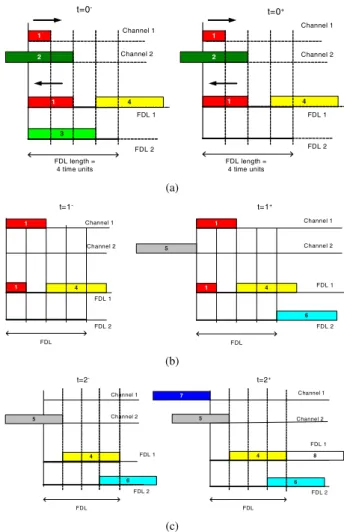
4 time units and no re-circulations, i.e., 𝜅 = 0. For illustrative purposes, all packets have the same size which is three time units. Consider the situation depicted in Fig. 1(a) at𝑡 = 0−.
On channel 1, packet 1 is under transmission upon a repeated attempt whereas on channel 2, packet 2 is under transmission upon its first attempt, therefore this packet is not using any FDL resources. The FDL 1 has the tail of packet 1 at its head but another packet 4 has just started to traverse through FDL 1 since it arrived one time unit ago but found both channels occupied. On FDL 2, packet 3 has just completed its journey on FDL 2 and is about to look for an opportunity to join one of the two wavelength channels. Since 𝜅 = 0 and
re-circulations are not allowed for this example and both channels are busy at 𝑡 = 0+, this packet 3 will be dropped by the
system leading to packet loss. Note that such a packet drop is specific to the PostRes reservation model since the output channel would not be reserved immediately when the packet
1 1 2 3 4 FDL length = 4 time units t=0 -1 1 2 4 t=0+ Channel 1 Channel 2 FDL 1 FDL 2 Channel 1 Channel 2 FDL 1 FDL 2 FDL length = 4 time units (a) 1 1 4 FDL t=1+ 5 6 Channel 1 Channel 2 FDL 1 FDL 2 1 1 4 FDL t=1 -Channel 1 Channel 2 FDL 1 FDL 2 (b) 4 FDL t=2+ 5 6 Channel 1 Channel 2 FDL 1 FDL 2 7 4 FDL t=2 -6 5 Channel 1 Channel 2 8 FDL 1 FDL 2 (c)
Fig. 1. The evolution of a feedback PostRes FDL buffer with 𝐾 = 2
wavelength channels and𝐵 = 2 FDLs each with length 𝐷 = 4 time units
where all packets have a length of three time units at three different time
epochs (a)𝑡 = 0, (b) 𝑡 = 1, (c) 𝑡 = 2. For a given time epoch 𝜏, packet
arrivals are said to occur at𝜏−and at time epoch𝜏+, decisions for these
packets, i.e., whether they are admitted to the wavelength channels or admitted to the FDL buffer or they are simply discarded, are made.
is accepted into the buffer in the PostRes model. Due to this packet drop, the system state is illustrated at 𝑡 = 0+ in the
right figure of Fig. 1(a). We let the system evolve until𝑡 = 1−
when two packets (numbered 5 and 6) arrive. The system state just before the arrivals is given in Fig. 1(b). Compared to Fig. 1(a), packet 2 has just left channel 2, the transmission of packet 1 over channel 1 and that of packet 4 over FDL 1 are in progress at𝑡 = 1−. Since at𝑡 = 1−, channel 2 is idle, one
of the arriving packets, say packet 5, would be accepted into channel 2, and the other arrival 6 would be directed to the idle FDL 2. The system state just after the arrivals is illustrated in the right figure of Fig. 1(b). We now let the system evolve until
𝑡 = 2− when three packets (numbered 7, 8, and 9) arrive. At
𝑡 = 2−, packet 7 is assigned to channel 1, packet 8 is directed
to FDL 1, but packet 9 finds both servers and FDLs busy and is dropped. The system state before and after these three arrivals is illustrated in Fig. 1(c). For this particular example, we used fixed packet sizes and instantaneous packet arrivals as in slotted systems only for illustrative purposes but the analytical model will be developed for asynchronous systems. Based on the operational principles outlined in Fig. 1, it
is not possible to exactly represent the system as a Markov process as in retrial queues. Therefore, it is clear that approx-imations are required for analyzing this system. Our approach is based on the stochastic characterization of the traffic coming out of the FDL buffer based on MMPP (Markov Modulated Poisson Process)-based models that have successfully been used in modeling overflow traffic in circuit-switched networks. An MMPP is characterized with a matrix pair(𝑄, 𝑅) where
𝑄 is the infinitesimal generator matrix of a modulating
finite-state continuous-time Markov chain and𝑅 = 𝑑𝑖𝑎𝑔{𝜆𝑖} is a
diagonal matrix of rates where𝜆𝑖 denotes the Poisson rate of
arrivals when the state 𝑖 of the modulating chain is visited
[28]. For more details on the properties of MMPPs, we refer the reader to [29]. Of particular interest to this paper is a two-state MMPP which has two two-states 1 and 2 with arrival rates
𝜆1 and𝜆2 in these two states, respectively. The transition rate
from state 1 to state 2 (state 2 to state 1) is denoted by𝜎1(𝜎2).
The two-state MMPP is then said to be characterized by the ordered quadruple(𝜆1, 𝜆2, 𝜎1, 𝜎2). In this paper, we assume
that the traffic coming out of the FDL buffer is modeled with a two-state MMPP called𝑋 comprising two states, namely
the HIGH and LOW states, which is characterized by the quadruple (𝑟𝐻, 𝑟𝐿, 𝜂, 𝛾). In the HIGH state, packet arrivals
are Poisson with rate 𝑟𝐻 and in the LOW state with rate 𝑟𝐿 such that 𝑟𝐻 ≥ 𝑟𝐿. The two-state MMPP 𝑋 is helpful
in representing the burstiness of this particular traffic stream while maintaining simplicity. We do not know the parameters of MMPP 𝑋 yet but we will obtain these parameters as an
outcome of an iterative process. However, this MMPP process is not independent from the channel occupancy process that keeps track of the number of busy channels at the designated port. This stems from the observation that a retrying optical packet will see a system quite correlated with the one the same packet had attempted to join but failed 𝐷 time units
back. For the purpose of characterizing this inter-dependence, let 𝑝𝑖,𝐻 (𝑝𝑖,𝐿) for 0 ≤ 𝑖 ≤ 𝐾 denote the joint probability that the two-state MMPP is in state HIGH (LOW) and there are 0 ≤ 𝑖 ≤ 𝐾 occupied channels at the designated port at an arbitrary epoch. Similarly, let 𝜋𝑖,𝐻 (𝜋𝑖,𝐿) denote the
probability that the two-state MMPP is in state HIGH (LOW) and there are0 ≤ 𝑖 ≤ 𝐾 occupied channels at the designated port at the epoch of an arbitrary retrial. Again, we do not know the probabilities 𝑝𝑖,𝐻, 𝑝𝑖,𝐿, 𝜋𝑖,𝐻, and 𝜋𝑖,𝐿 at this point but
we will obtain these probabilities through the same iterative procedure. Moreover, we define
𝑝𝐻 = 𝐾 ∑ 𝑖=0 𝑝𝑖,𝐻, 𝑝𝐿= 𝐾 ∑ 𝑖=0 𝑝𝑖,𝐿, 𝜋𝐻= 𝐾 ∑ 𝑖=0 𝜋𝑖,𝐻, 𝜋𝐿= 𝐾 ∑ 𝑖=0 𝜋𝑖,𝐿.
Let us now define the bi-variate process 𝒳 (𝑡) = {(𝐶𝑃(𝑡), 𝑆𝑃(𝑡)); 𝑡 ≥ 0}, where 0 ≤ 𝐶𝑃(𝑡) ≤ 𝐾 denotes
the number of busy channels at the designated port and
𝑆𝑃(𝑡) ∈ {𝐻, 𝐿} denotes the state of the two-state MMPP 𝑋 (whether it is in the HIGH or LOW state) at time 𝑡.
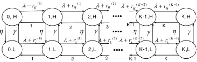
The rate of repeated (i.e., retrying) arrivals when𝐶𝑃(𝑡) = 𝑖 and 𝑆𝑃(𝑡) = 𝐻 is denoted by 𝑟𝐻(𝑖), 0 ≤ 𝑖 ≤ 𝐾. Note that 𝑟𝐻(𝑖) should be proportional with 𝜋𝑖,𝐻/𝜋𝐻 and moreover it
should hold that 𝑝𝐻𝑟𝐻 = ∑𝐾𝑖=0𝑝𝑖,𝐻𝑟𝐻(𝑖). From these two
(0 ) H r λ+ (1) H r λ+ ( 2) H r λ+ (K 2) H r λ+ − (K1) H r λ+ − ( 0) L r λ+ (1) L r λ+ ( 2 ) L r λ+ (K2 ) L r λ+ − (K1) L r λ+ − η γ 1 η η γ 1 2 2 3 3 K-1 K K K-1 η γ η γ γ 0, H 1,H 2,H K-1,H K,H 0,L 1,L 2,L K-1,L K,L
Fig. 2. The transition diagram of the Markov chain governing the behavior
of the bi-variate process𝒳 (𝑡).
observations, we conclude that
𝑟(𝑖)𝐻 = 𝑟𝐻𝑝𝐻𝜋𝑖,𝐻𝜋𝐻𝑝𝑖,𝐻. (1)
Similarly, if we define 𝑟(𝑖)𝐿 , 0 ≤ 𝑖 ≤ 𝐾, to be the rate of
repeated arrivals when𝐶𝑃(𝑡) = 𝑖 and 𝑆𝑃(𝑡) = 𝐿, we obtain
𝑟𝐿(𝑖) = 𝑟𝐿𝑝𝜋𝐿𝑝𝑖,𝐿𝐿𝜋𝑖,𝐿. (2)
Assuming that retrials at a given state of𝒳 (𝑡) are of Poisson
nature, we have a continuous-time Markov chain of size 2(𝐾 + 1) whose transition diagram is given in Fig. 2 which approximates the behavior of the occupancy process of the port, called hereafter the port process.
By definition, the probabilities we defined 𝑝𝑖,𝐻 and 𝑝𝑖,𝐿
for 0 ≤ 𝑖 ≤ 𝐾 are the steady-state probabilities of the port process described by its state-transition diagram in Fig. 2. Let
𝑃 denote the infinitesimal generator of this Markov chain with
the states enumerated as
{(0, 𝐻), (1, 𝐻), . . . , (𝐾, 𝐻), (0, 𝐿), . . . , (𝐾, 𝐿)}.
Packets are blocked and directed to the FDL buffer only in the two states (𝐾, 𝐻) and (𝐾, 𝐿). In particular, the rate of traffic directed to the FDL buffer is𝜆+ 𝑟(𝐾)𝐻 𝜅 at state (𝐾, 𝐻)
and 𝜆 + 𝑟𝐿(𝐾)𝜅 at state (𝐾, 𝐿). Assuming an MMPP model,
the traffic comprising packets directed to the FDL buffer can be modeled with an MMPP with 2(𝐾 + 1) states with infinitesimal generator𝑃 and rate matrix
𝑅 = diag{[0, . . . , 0, 𝜆 + 𝑟(𝐾)𝐻 𝜅, 0, . . . , 0, 𝜆 + 𝑟(𝐾)𝐿 𝜅]}. (3)
Although a large-scale MMPP model with2(𝐾 + 1) states is now at hand, we propose to further use the model reduction algorithm of [26] to reduce this MMPP characterized with the pair (𝑃, 𝑅) to a two-state MMPP denoted by 𝑌 . The algorithm proposed in [26] for model reduction matches the first three marginal moments and the area under the auto-covariance function of the original process to those of the two-state approximating MMPP 𝑌 . This particular algorithm
is given in Appendix A for the sake of completeness. The
MMPP 𝑌 is assumed to be characterized with the quadruple
(𝑟1, 𝑟2, 𝜂1, 𝛾1).
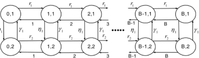
We have now obtained a stochastic characterization of the traffic appearing at the input of the FDL buffers. However, some of the packets directed to the FDL buffer will not be admitted due to the lack of an idle FDL. In order to find a characterization for the actual traffic carried through the FDL buffer, we define another bi-variate process 𝒴(𝑡) = {(𝐶𝐹(𝑡), 𝑆𝐹(𝑡)); 𝑡 ≥ 0}, where 0 ≤ 𝐶𝐹(𝑡) ≤ 𝐵 denotes the
0,1 1,1 2,1 B-1,1 B,1 0,2 1,2 2,2 B-1,2 B,2 1 η γ1 η1 γ1 η1 γ1 η1 γ1 η1 γ1 1 2 B-1 B 1 2 3 3 B -1 B 1 r r1 r1 r1 r1 2 r r2 r2 r2 r2
Fig. 3. The transition diagram of the Markov chain governing the behavior
of the bi-variate process𝒴(𝑡).
denotes the state of the two-state MMPP 𝑌 at time 𝑡. We
then have a continuous-time Markov chain of size 2(𝐵 + 1) whose transition diagram is given in Fig. 3 which hereafter is referred to as the buffer process. Let𝑄 denote the infinitesimal
generator of this buffer process with the states enumerated as
{(0, 0), (1, 1), . . . , (𝐵, 1), (0, 2), . . . , (𝐵, 2)}. Packets are not
admitted into the buffer only in the two states (𝐵, 1) and (𝐵, 2). In particular, the rate of traffic using the FDL buffer is 𝑟1 at state (𝑖, 1) and 𝑟2 at state (𝑖, 2) for all 𝑖 such that
0 ≤ 𝑖 < 𝐵. Assuming an MMPP model, the traffic comprising packets using the FDL buffer can be modeled with an MMPP with2(𝐵 + 1) states with infinitesimal generator 𝑄 and rate matrix
Λ = diag{[𝑟1, . . . , 𝑟1, 0, 𝑟2, . . . , 𝑟2, 0]}. (4)
We again use the procedure of [26] for reducing this MMPP to a two-state MMPP say 𝑍 which is characterized by the
quadruple(ˆ𝑟𝐻, ˆ𝑟𝐿, 𝜂, 𝛾) such that ˆ𝑟𝐻 ≥ ˆ𝑟𝐿. Moreover, let 𝑞
denote the steady-state vector of𝑄:
𝑞 = [𝑞0,1, . . . , 𝑞𝐵,1, 𝑞0,2, . . . , 𝑞𝐵,2]. (5)
Let us now revisit the port process whose transition diagram was given in Fig. 2. Blocking arises when an arriving packet finds the system in one of the two states(𝐾, 𝐻) and (𝐾, 𝐿). A blocked packet should have visited the state (𝐾, 𝐻) with probability𝛼𝐻 and state(𝐾, 𝐿) with probability 𝛼𝐿:
𝛼𝐻 = (𝜆 + 𝑟 (𝐾) 𝐻 𝜅)𝑝𝐾,𝐻 (𝜆 + 𝑟(𝐾)𝐻 𝜅)𝑝𝐾,𝐻+ (𝜆 + 𝑟(𝐾)𝐿 𝜅)𝑝𝐾,𝐿 , 𝛼𝐿= 1 − 𝛼𝐻. (6) Assume that the initial distribution of the Markov chain in Fig. 2 is given by the row vector
𝜋0= [0, . . . , 0, 𝛼𝐻, 0, . . . , 0, 𝛼𝐿]. (7)
Then, it is clear that the vector defined by
𝜋 = 𝜋0𝑒𝑄𝐷 (8)
gives the conditional probabilities𝜋𝑖,𝐻 and𝜋𝑖,𝐿 such that
𝜋 = [𝜋0,𝐻, . . . , 𝜋𝐾,𝐻, 𝜋0,𝐿, . . . , 𝜋𝐾,𝐿]. (9)
We now have to link the two-state MMPP𝑍 to the MMPP 𝑋. Let us consider the two extreme cases as the FDL delay 𝐷 → ∞ and 𝐷 → 0. As 𝐷 → ∞, the traffic coming out
of the FDL buffer should be independent of the port process. Note that𝜋 → 𝑝 as 𝐷 → ∞ where
𝑝 = [𝑝0,𝐻, . . . , 𝑝𝐾,𝐻, 𝑝0,𝐿, . . . , 𝑝𝐾,𝐿] (10)
and therefore𝑟(𝐻)𝑖 → 𝑟𝐻 and 𝑟(𝐿)𝑖 → 𝑟𝐿. Consequently, as
𝐷 → ∞, 𝑟𝐻 and𝑟𝐿 should be chosen so that𝑟𝐻 = ˆ𝑟𝐻 and
TABLE I
ITERATIVE ALGORITHM FOR FINDING VARIOUS PERFORMANCE
MEASURES OF THEFDLBUFFERING SYSTEM
Input:𝐾, 𝐵, 𝐷, 𝜅
1. First start with arbitrary probability vectors𝑝 and 𝜋 as well as the
two-state MMPP𝑋 with zero rates in each state with arbitrary 𝜂
and𝛾.
2. Given the vectors𝑝 and 𝜋 and the parameters 𝑟𝐻,𝑟𝐿,𝜂, and 𝛾,
construct the Markov chain depicted in Fig. 2 with generator𝑃 and
solve for its steady-state probability vector𝑝 which in turn gives
the probabilities𝑝𝑖,𝐻 and𝑝𝑖,𝐿for0 ≤ 𝑖 ≤ 𝐾.
3. Find the vector𝜋 from (8) and define the rate matrix 𝑅 as in (3).
4. Use the procedure in Appendix A to obtain the two-state MMPP
model𝑌 characterized by the quadruple (𝑟1, 𝑟2, 𝜂1, 𝛾1) from the
2(𝐾 +1)− dimensional MMPP characterized with the pair (𝑃, 𝑅).
5. Given the parameters𝑟1,𝑟2,𝜂1, and𝛾1, construct the Markov chain
depicted in Fig. 3 with generator𝑄 and solve for its steady-state
probability vector𝑞.
6. First define the rate matrixΛ as in (4) and use the procedure in
Appendix A to obtain the two-state MMPP model𝑍 given from the
2(𝐵 +1)− dimensional MMPP characterized with the pair (𝑄, Λ).
7. Employ (11) to update𝑟𝐻 and𝑟𝐿which completes the
character-ization of the MMPP𝑋 since the parameters 𝜂 and 𝛾 are already
obtained in the previous step.
8. If the normalized difference between two successive values of the
vector𝑝 is less than a tolerance parameter 𝜀, then exit the loop.
9. Go to step 2.
Output: loss probability𝑃𝐿, expected delay𝐸[𝑊 ], etc.
𝑟𝐿 = ˆ𝑟𝐿. Consequently, the Markov chain in Fig. 2 reduces
to the modeling of a𝐾-server system fed with Poisson traffic
with rate 𝜆 and independent MMPP 𝑍 traffic coming out of
the FDL buffer. The situation is different as 𝐷 → 0 since
the traffic retrying to join the port is completely dependent on the port process and the burstiness of this stream should not play any additional role. Therefore, as 𝐷 → 0, we propose
to replace the MMPP𝑍 with a pure Poisson process with the
same average rate, i.e.,𝑟𝐻= 𝑟𝐿= ˆ𝑟𝐻𝛾+ˆ𝑟𝜂+𝛾𝐿𝜂. We now have a
way of characterizing the traffic coming out of the FDL buffer in the two extreme scenarios. For arbitrary values of 𝐷, we
propose the following adjustment:
𝑟𝐻 = ˆ𝑟𝐿+ (ˆ𝑟𝐻− ˆ𝑟𝐿)(1 − 𝛽) + (ˆ𝑟𝐻− ˆ𝑟𝐿)𝛽𝜂 + 𝛾𝛾 , 𝑟𝐿 = ˆ𝑟𝐿+ (ˆ𝑟𝐻− ˆ𝑟𝐿)𝛽𝜂 + 𝛾𝛾 , (11)
where𝛽 = ∣∣𝜋 − 𝑝∣∣2/∣∣𝜋0− 𝑝∣∣2, where ∣∣𝑥∣∣2 is the 2-norm
of the vector 𝑥, i.e., square root of the sum of the squares
of the entries of the vector 𝑥. It is also well-known that 𝛽
approaches zero exponentially fast as𝐷 → ∞ . This method
ensures that the average rate of the MMPP 𝑋 matches the
average rate of MMPP𝑍 for all choices of 𝛽 whereas the two
MMPPs are exactly the same as 𝐷 → ∞ as desired but the
approximate MMPP is replaced with a Poisson process with the same average rate as𝐷 → 0. The method described above
leads us to a fixed-point iterative procedure which is provided in Table I.
The most important performance measure of interest is the loss probability 𝑃𝐿 which is the probability that a packet is dropped by the system. Upon convergence of the algorithm given in Table I, we write 𝑃𝐿 as follows:
𝑃𝐿= (𝑟
(𝐾)
𝐻 𝑝𝐾,𝐻 + 𝑟(𝐾)𝐿 𝑝𝐾,𝐿)(1 − 𝜅) + 𝑟1𝑞𝐵,1+ 𝑟2𝑞𝐵,2
On the other hand, the mean waiting time in the system is given by 𝐸[𝑊 ] where 𝑊 denotes the waiting time of a
successfully transmitted packet. It is not difficult to show that
𝐸[𝑊 ] = 𝐷𝑟𝑓𝑠𝑟
(1−𝑃𝐿)(1−𝑟𝑟2), where 𝑟𝑓 is the probability that a fresh arrival uses the FDL buffer, i.e., packet retries at least once,
𝑠𝑟is the probability that a retrial attempt is successful, and𝑟𝑟
is the probability that a retrial attempt leads to another retrial, i.e., retrying packet finds all channels occupied, therefore gets directed to the FDL buffer, and finds one idle FDL. We write these probabilities below:
𝑟𝑓 = (𝑝𝐾,𝐻+ 𝑝𝐾,𝐿) ∑𝐵−1 𝑖=0 (𝑟1𝑞𝑖,1+ 𝑟2𝑞𝑖,2) 𝑟1𝛾1+𝑟2𝜂1 𝜂1+𝛾1 , 𝑠𝑟 = ∑𝐾−1 𝑖=0 (𝑟𝐻(𝑖)𝑝𝑖,𝐻+ 𝑟(𝑖)𝐿 𝑝𝑖,𝐿) ˆ𝑟𝐻𝛾+ˆ𝑟𝐿𝜂 𝜂+𝛾 , 𝑟𝑟 = 𝜅(𝑟(𝐾)𝐻 𝑝𝐾,𝐻+ 𝑟𝐿(𝐾)𝑝𝐿,𝐻) ˆ𝑟𝐻𝛾+ˆ𝑟𝐿𝜂 𝜂+𝛾 ∑𝐵−1 𝑖=0 (𝑟1𝑞𝑖,1+ 𝑟2𝑞𝑖,2) 𝑟1𝛾1+𝑟2𝜂1 𝜂1+𝛾1 .
Another performance measure we are interested in is the probability of strictly more than𝑁 circulations for a successful
packet which is denoted by 𝑃𝑅(𝑁) = 𝑃 [𝑊 > 𝑁𝐷]. We
can write this probability as𝑃𝑅(𝑁) = 𝑟𝑓𝑠𝑟𝑟
𝑁 𝑟
(1−𝑃𝐿)(1−𝑟𝑟). Finally, the computational complexity of the proposed method per iteration is 𝑂(𝑀3) where 𝑀 = max(𝐾, 𝐵) which is quite
reasonable when compared to traditional multi-dimensional retrial queues.
III. NUMERICALRESULTS
We validate the accuracy of the proposed approach by comparing them against simulations. The iteration tolerance parameter is set to𝜀 = 0.000001 throughout all the numerical
examples. As a first example, we fix 𝐾 = 16, 𝜌 = 0.6 and 𝜅 = 0 (i.e., only one FDL circulation is allowed). We then
plot the loss probability𝑃𝐿 as a function of the FDL delay
𝐷 in Fig. 4 obtained through simulations and the approach
proposed in this article. For comparison purposes, we also test three other methods:
∙ Method A: This method is the same as the proposed
algorithm except that the adjustment proposed in (11) is not made and we therefore set𝑟𝐻= ˆ𝑟𝐻 and𝑟𝐿= ˆ𝑟𝐿
irrespective of the FDL delay𝐷.
∙ Method B: Instead of modeling the traffic directed to
the FDL buffer as a two-state MMPP, we use a Poisson process with the same average rate and therefore ignore the burstiness of this traffic stream.
∙ Method C: This method is the M/M/K/K+B traditional
queuing model also described in [14] in the context of FDL buffers.
The results are depicted in Fig. 4. We have several observa-tions:
∙ For this example, the loss probability 𝑃𝐿 appears to
saturate beyond𝐷 = 2 and there appears to be minimal
need to further increase FDL lengths since the loss probability would not reduce much. This observation is consistent with the observation of [12] on required FDL delays based on simulation only.
0 0.5 1 1.5 2 10−3 10−2 10−1 Loss Probability P L a) B=4 FDL Delay D 0 0.5 1 1.5 2 10−6 10−5 10−4 10−3 10−2 Loss Probability P L b) B=16 FDL Delay D simulation analysis method A method B method C simulation analysis method A method B method C
Fig. 4. Loss probability 𝑃𝐿 as a function of the FDL delay 𝐷 for the
particular case𝐾 = 16, 𝜌 = 0.6, 𝜅 = 0.
∙ MMPP-based models accurately estimate the loss
prob-ability in the asymptotic regime of 𝐷 → ∞ as opposed
to Poisson process-based models, i.e., Method B, that come short of capturing the burstiness of the traffic stream associated with retrials.
∙ Method C provides very loose lower bounds on the loss
probability especially for larger𝐵 and it is evident that
the traditional M/M/K/K+B based queuing models can not effectively be used for dimensioning FDL buffers.
∙ The adjustment of MMPP parameters proposed in (11)
is especially useful for relatively small FDL delays and improves accuracy with respect to Method A that does not employ this adjustment procedure.
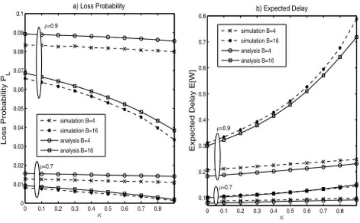
In the next example, we fix 𝐾 = 16 and 𝐷 = 2, and
we plot the loss probability𝑃𝐿 and expected delay𝐸[𝑊 ] for
two different values of𝐵 in Fig. 5a and Fig. 5b, respectively,
for 𝜌 = 0.7 and 𝜌 = 0.9, as a function of the re-circulation
parameter 𝜅. It is clear that the proposed analysis method
accurately captures the behavior of the system as a function of the re-circulation parameter𝜅 as well as the other parameters
such as 𝜌 and 𝐵 although we note the existence of a slight
discrepancy between the results of simulations and analysis. The major factors for this discrepancy are the reduced order MMPP modeling of the actual traffic directed to the FDL buffer for computational feasibility and the inter-dependence between the port and buffer processes that is ignored.
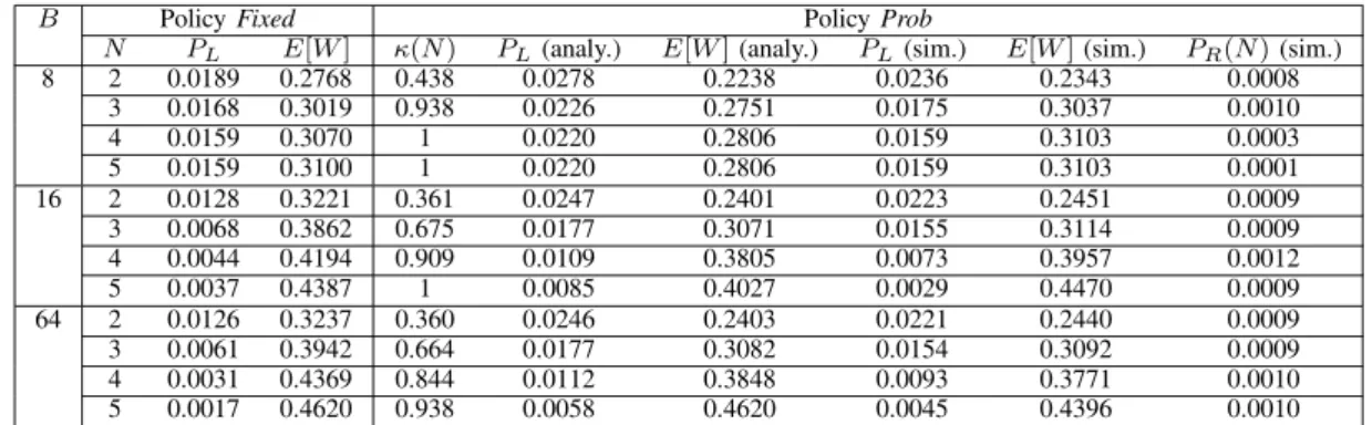
In the current example, we compare two policies of re-circulation control; Policy Fixed allowing a fixed number of circulations (𝑁 circulations at most) as in [15] and Policy Prob using probabilistic re-circulation as proposed and studied
in the current article. Policy Fixed is commonly proposed in the literature since a limit is placed on the number of FDL circulations in order not to require signal regeneration. In order to compare against Policy Fixed with𝑁 allowable circulations,
0 0.1 0.2 0.3 0.4 0.5 0.6 0.7 0.8 0 0.01 0.02 0.03 0.04 0.05 0.06 0.07 0.08 0.09 0.1 κ Loss Probability P L a) Loss Probability 0 0.1 0.2 0.3 0.4 0.5 0.6 0.7 0.8 0.1 0.2 0.3 0.4 0.5 0.6 0.7 0.8 κ
Expected Delay E[W]
b) Expected Delay simulation B=4 simulation B=16 analysis B=4 analysis B=16 simulation B=4 simulation B=16 analysis B=4 analysis B=16 ρ=0.9 ρ=0.7 ρ=0.9 ρ=0.7
Fig. 5. Loss probability𝑃𝐿and expected delay𝐸[𝑊 ] as a function of the
re-circulation parameter𝜅 for 𝐾 = 16, 𝐷 = 2, and for two different values
of𝐵 and 𝜌.
by analysis (using binary search) such that 𝑃𝑅(𝑁) is small enough. In this example, we set 𝑃𝑅(𝑁) = 0.001. In case this identity can not be satisfied, we set 𝜅(𝑁) = 1. In this
way, we place a statistical limit on the maximum number of FDL circulations with Policy Prob. We report our findings in Table II for the case𝐾 = 16, 𝐷 = 2, 𝜌 = 0.8, and for various
values of the buffer size𝐵. Note that only simulation results
are reported for Policy Fixed whereas we have both analysis and simulation results for Policy Prob. We have the following observations:
∙ Table II clearly demonstrates that the analysis method is
able to capture the performance measure𝑃𝑅(𝑁); note the
last column obtained via simulations with𝑃𝑅(𝑁) values
very close to0.001 as desired when 𝜅 < 1.
∙ For𝜅(𝑁) < 0.9, the analysis method gives quite accurate
results when compared to simulations for all three perfor-mance measures we studied. However, accuracy appears to be reduced when𝜅(𝑁) is closer to unity.
∙ Although policies Fixed and Prob present comparable 𝑃𝑅(𝑁), the way we select 𝜅(𝑁) leads to slightly larger loss probability 𝑃𝐿 but slightly lower delay 𝐸[𝑊 ] for
Policy Prob when compared to Policy Fixed for a given
𝑁 for 𝜅(𝑁) < 1. This situation appears to be slightly
reversed when𝜅(𝑁) = 1. When 𝜅(𝑁) < 1, in order to
reduce the loss probability for Policy Prob, one needs to further increase 𝜅(𝑁) which however also increases 𝑃𝑅(𝑁). The results show that Policy Fixed outperforms
Policy Prob if a delay constraint is given in terms of
𝑃𝑅(𝑁) only but there are scenarios for which Policy Prob may outperform Policy Fixed when there are further
constraints on delay for example in terms of 𝐸[𝑊 ].
Another advantage of probabilistic circulation is the existence of infinitely many choices for𝜅 as opposed to
a few values for𝑁 to choose from, to optimize system
behavior in terms of𝑃𝐿,𝐸[𝑊 ], and 𝑃𝑅(𝑁).
In the next example, for a given parameter set(𝐾, 𝐷, 𝐵, 𝜅), we find the maximum load𝜌𝑚(𝐾, 𝐷, 𝐵, 𝜅), so-called through-put, on the associated system that meets the specific QoS requirements, i.e., 𝑃𝐿 ≤ 𝑘𝐿, 𝑃𝑅(𝑁) ≤ 𝑘𝑅(𝑁), 𝐸[𝑊 ] ≤ 𝑘𝑊.
To obtain the quantity 𝜌𝑚(𝐾, 𝐷, 𝐵, 𝜅), we iteratively vary
the load on the system and use the proposed analysis method
5 10 15 20 25 30 1 32 0.58 0.6 0.62 0.64 0.66 0.68 0.7 0.72 0.5689 Buffer Size B Throughput κ= 0, D = 0.5 κ= 0.5, D = 0.5 κ= 0.9, D = 0.5 κ= 0, D = 1 κ= 0, D = 2 κ= 0.5, D = 1 κ= 0.5, D = 2 κ= 0.9, D = 1 κ= 0.9, D = 2 Erlang-B
Fig. 6. The throughput of the system as a function of𝐵 for the case 𝐾 = 32
and for three different values of𝜅 and 𝐷
until all QoS requirements are just met. The low computational complexity of the analysis method allows us to obtain the quantity𝜌𝑚(𝐾, 𝐷, 𝐵, 𝜅) for a wide range of problem
param-eters in acceptable time. For this example, we fix 𝐾 = 32, 𝑘𝐿 = 0.001, 𝑁 = 3, 𝑘𝑅(3) = 0.001, and 𝑘𝑊 = 0.02.
Note that the expected delay requirement is relatively strict for this example. We then plot the throughput of the system as a function of𝐵 for 𝜅 = 0, 0.5, 0.9 and for 𝐷 = 0.5, 1, 2 in
Fig. 6. If no buffers are used, we obtain the throughput of the system as 0.5689 using the Erlang-B formula which is also plotted in Fig. 6 as a lower bound. Our goal in this example is to quantify the gain in throughput by using FDL buffers but still meeting the QoS requirements of the system. If there are no delay or re-circulation constraints, one can increase𝐵
and𝜅 together to arbitrarily increase the throughput but at the
expense of very high expected delays. In this example, delay and re-circulation constraints are also taken into account. For small𝐷, the throughput increases monotonically with respect
to𝐵 and 𝜅 since the delay and re-circulation constraints are
not violated for all parameters we tried. However, for larger values of𝐷, the throughput increases until a certain value of 𝐵
and then starts to decrease for fixed𝜅. A similar argument can
be made for larger values of𝜅 for which throughput is reduced
beyond a certain value of𝜅 for large 𝐷. This observation leads
us to the conclusion that provisioning optical buffers requires analysis and optimization on provisioning parameters such as
𝐵, 𝜅, and 𝐷.
In our final example, we fix 𝐾 = 32 and 𝜅 = 0.9 and
searched for the optimum value of𝐷, say 𝐷𝑜𝑝𝑡, in the interval
0.2 ≤ 𝐷 ≤ 4 that yields the maximum throughput denoted by 𝜌𝑜𝑝𝑡 as a function of the delay requirement𝑘𝑊. For this
example, we set𝑘𝐿= 0.001, 𝑁 = 3, and 𝑘𝑅(3) = 0.001. The
results are given for three different choices of𝐵 in Table III.
The results show that increasing the buffer size𝐵 beyond 𝐾 is
not very helpful. The maximum throughput strictly depends on the delay requirement whereas the optimum delay 𝐷𝑜𝑝𝑡
increases with increasing delay requirement𝑘𝑊 as expected but decreases with buffer size𝐵.
IV. CONCLUSION
We propose a retrial-queuing model along with fixed-point iterations to evaluate the performance of multi-wavelength feedback FDL optical buffers. Simulation results show that
TABLE II
COMPARISON OFPOLICIESFixedANDProbFOR THE CASE𝐾 = 16, 𝐷 = 2, 𝜌 = 0.8,AND FOR VARIOUS VALUES OF THE BUFFER SIZE𝐵 = 8, 16, 64.
BOTH ANALYSIS AND SIMULATION RESULTS ARE REPORTED FORPOLICYProb.
𝐵 Policy Fixed Policy Prob
𝑁 𝑃𝐿 𝐸[𝑊 ] 𝜅(𝑁) 𝑃𝐿(analy.) 𝐸[𝑊 ] (analy.) 𝑃𝐿(sim.) 𝐸[𝑊 ] (sim.) 𝑃𝑅(𝑁) (sim.)
8 2 0.0189 0.2768 0.438 0.0278 0.2238 0.0236 0.2343 0.0008 3 0.0168 0.3019 0.938 0.0226 0.2751 0.0175 0.3037 0.0010 4 0.0159 0.3070 1 0.0220 0.2806 0.0159 0.3103 0.0003 5 0.0159 0.3100 1 0.0220 0.2806 0.0159 0.3103 0.0001 16 2 0.0128 0.3221 0.361 0.0247 0.2401 0.0223 0.2451 0.0009 3 0.0068 0.3862 0.675 0.0177 0.3071 0.0155 0.3114 0.0009 4 0.0044 0.4194 0.909 0.0109 0.3805 0.0073 0.3957 0.0012 5 0.0037 0.4387 1 0.0085 0.4027 0.0029 0.4470 0.0009 64 2 0.0126 0.3237 0.360 0.0246 0.2403 0.0221 0.2440 0.0009 3 0.0061 0.3942 0.664 0.0177 0.3082 0.0154 0.3092 0.0009 4 0.0031 0.4369 0.844 0.0112 0.3848 0.0093 0.3771 0.0010 5 0.0017 0.4620 0.938 0.0058 0.4620 0.0045 0.4396 0.0010 TABLE III
THE VALUES𝐷𝑜𝑝𝑡AND𝜌𝑜𝑝𝑡AS A FUNCTION OF THE DELAY
REQUIREMENT𝑘𝑊 FOR𝐾 = 32AND𝜅 = 0.9AND FOR THREE VALUES
OF𝐵. 𝐵 Delay Requirement𝑘𝑊 𝐷𝑜𝑝𝑡 𝜌𝑜𝑝𝑡 16 0.005 0.28 0.6774 0.01 0.73 0.6881 0.02 1.00 0.7118 0.05 1.68 0.7397 0.1 2.93 0.7509 0.2 4.00 0.7527 32 0.005 0.30 0.6933 0.01 0.53 0.7039 0.02 0.72 0.7251 0.05 1.18 0.7562 0.1 2.05 0.7702 0.2 3.92 0.7766 64 0.005 0.20 0.7095 0.01 0.40 0.7188 0.02 0.62 0.7324 0.05 1.15 0.7574 0.1 2.03 0.7706 0.2 3.89 0.7750
the proposed model allows one to accurately estimate the loss probabilities, expected delays, and re-circulation probabilities in this system. Provisioning procedures based on the analytical model we develop are also presented to validate the effective-ness of the proposed approach. We leave the queuing modeling of shared FDL feedback buffers and the alternative scenario of employing a fixed limit on the number of FDL circulations for future research.
APPENDIXA
TWO-STATEMMPPAPPROXIMATION
One of the crucial components of the proposed method in this article is a two-state MMPP approximation characterized with the pair(𝐴, Λ) to an original MMPP characterized with the pair(𝑄, 𝑅) with 𝑛 > 2 states. Let
𝐴 = [ −𝜎1 𝜎1 𝜎2 −𝜎2 ] , Λ = [ 𝜆1 0 0 𝜆2 ] .
Also let 𝑥 denote the steady-state vector of the modulating
Markov chain such that 𝑥𝑄 = 0, 𝑥𝑒 = 1 where 𝑒 denotes
a column vector of ones of appropriate size. The𝑟th central
moment of the arrival rate of the original MMPP is denoted
by 𝑚𝑟 and is given by𝑚𝑟 = 𝑥𝑅𝑟𝑒, 𝑟 ≥ 1. Let 𝑣 denote the
variance of the original MMPP that is given by𝑣 = 𝑚2−𝑚21.
The time constant 𝜏𝑐 of the original MMPP is expressed as
𝜏𝑐 = 1
𝑣
∫∞
0 𝑟(𝑡)𝑑𝑡, where 𝑟(𝑡) is the covariance function of
the arrival rate. The reference [27] gives an expression for𝜏𝑐:
𝜏𝑐=𝑣1[𝑥𝑅(𝑒𝑥 − 𝑄)−1𝑅𝑒 − 𝑚2 1].
The following choices for the parameters of the approximating MMPP are known to match the first three non-central moments as well as the time constant [26]:
𝜎1= 𝜏𝑐(1 + 𝜂)1 , 𝜎2=𝜏𝑐(1 + 𝜂)𝜂 , 𝜆1= 𝑚1+ √ 𝑣/𝜂, 𝜆2= 𝑚1−√𝑣𝜂, where 𝜂 = 1 + 𝛿 2(𝛿 − √ 4 + 𝛿2), 𝛿 = 𝑚3− 3𝑚1𝑣 − 𝑚31 𝑣3/2 . ACKNOWLEDGMENT
This work is done when Nail Akar was visiting UMKC as a Fulbright research scholar. The work of Nail Akar was supported in part by the support of the BONE-project (“Building the Future Optical Network in Europe”), a Network of Excellence funded by the European Commission through the 7th ICT-Framework Programme.
REFERENCES
[1] P. Gambini, M. Renaud, C. Guillemot, F. Callegati, I. Andonovic, B. Bostica, D. Chiaroni, G. Corazza, S. L. Danielsen, P. Gravey, P. B. Hansen, M. Henry, C. Janz, A. Kloch, R. Krahenbuhl, C. Raf-faelli, M. Schilling, A. Talneau, and L. Zucchelli, “Transparent optical packet switching: network architecture and demonstrators in the KEOPS project," IEEE J. Sel. Areas Commun., vol. 16, pp. 1245–1259, 1998. [2] C. Qiao and M. Yoo, “Optical burst switching (OBS)–a new paradigm
for an optical Internet," J. High Speed Netw., vol. 8, no. 1, pp. 69–84, 1999.
[3] F. Callegati, W. Cerroni, G. Corazza, C. Develder, M. Pickavet, and P. Demeester, “Scheduling algorithms for a slotted packet switch with either fixed or variable length packets," Photonic Netw. Commun., vol. 8, no. 2, pp. 163–176, 2004.
[4] W. A. Vanderbauwhede and D. A. Harle, “Architecture, design, and modeling of the OPSnet asynchronous optical packet switching node," J. Lightwave Technol., vol. 23, pp. 2215–2228, 2005.
[5] O. Ozturk, E. Karasan, and N. Akar, “Performance evaluation of slotted optical burst switching systems with quality of service differentiation," J. Lightwave Technol., vol. 27, no. 14, pp. 2621–2633, 2009.
[6] R. Barry and P. Humblet, “Models of blocking probability in all-optical networks with and without wavelength changers," IEEE J. Sel. Areas Commun., vol. 14, no. 5, pp. 858–867, June 1996.
[7] I. Chlamtac, A. Fumagalli, L. Kazovsky, P. Melman, W. Nelson, P. Poggiolini, M. Cerisola, A. Choudhury, T. Fong, R. Hofmeister, C.-L. Lu, A. Mekkittikul, I. Sabido, D. J. M., C.-J. Suh, and E. Wong, “Cord: contention resolution by delay lines," IEEE J. Sel. Areas Commun., vol. 14, no. 5, pp. 1014–1029, June 1996.
[8] R. S. Tucker, P.-C. Ku, and C. J. Chang-Hasnain, “Slow-light optical buffers: capabilities and fundamental limitations," Lightwave Technol., J., vol. 23, no. 12, pp. 4046–4066, Dec. 2005.
[9] D. Hunter, M. Chia, and I. Andonovic, “Buffering in optical packet switches," J. Lightwave Technol., vol. 16, no. 12, pp. 2081–2094, Dec 1998.
[10] W. D. Zhong and R. S. Tucker, “Wavelength routing-based photonic packet buffers and their applications in photonic packet switching systems," J. Lightwave Technol., vol. 16, no. 10, pp. 1737–1745, Oct. 1998.
[11] L. Xu, H. Perros, and G. Rouskas, “Techniques for optical packet switching and optical burst switching," IEEE Commun. Mag., vol. 39, no. 1, pp. 136–142, Jan. 2001.
[12] C. M. Gauger, “Dimensioning of FDL buffers for optical burst switching nodes," in Proc. 6th IFIP Working Conference on Optical Network Design and Modelling, Feb. 2002.
[13] F. Callegati, “Optical buffers for variable length packets," IEEE Com-mun. Lett., vol. 4, no. 9, pp. 292–294, Sep. 2000.
[14] J. S. Turner, “Terabit burst switching," J. High Speed Netw. (JHSN), vol. 8, no. 1, pp. 3–16, 1999.
[15] A. Rostami and S. Chakraborty, “On performance of optical buffers with specific number of circulations," IEEE Photonics Technol. Lett., vol. 17, no. 7, pp. 1570–1572, 2005.
[16] W. Rogiest, J. Lambert, D. Fiems, B. van Houdt, H. Bruneel, and C. Blondia, “A unified model for synchronous and asynchronous FDL buffers allowing closed-form solution," Performance Evaluation, vol. 66, no. 7, pp. 343–355, 2009.
[17] W. Rogiest and H. Bruneel, “Exact optimization method for an FDL buffer with variable packet length," IEEE Photon. Technol. Lett., vol. 22, no. 4, pp. 242–244, 2011.
[18] J. Almeida, J. Pelegrini, and H. Waldman, “A generic-traffic optical buffer modeling for asynchronous optical switching networks," IEEE Commun. Lett., vol. 9, no. 2, pp. 175–177, Feb. 2005.
[19] H. Kankaya and N. Akar, “Exact analysis of single-wavelength optical buffers with feedback Markov fluid queues," IEEE/OSA J. Optical Commun. Netw., vol. 1, no. 6, pp. 530–542, Nov. 2009.
[20] M. Yoo, C. Qiao, and S. Dixit, “QoS performance of optical burst switching in IP-over-WDM networks," IEEE J. Sel. Areas Commun., vol. 18, pp. 2062–2071, Oct. 2000.
[21] X. Lu and B. Mark, “Performance modeling of optical-burst switching with fiber delay lines," IEEE Trans. Commun., vol. 52, no. 12, pp. 2175– 2183, Dec. 2004.
[22] J. R. Artalejo and A. Gomez-Corral, Retrial Queueing Systems. Springer, 2008.
[23] T. Yang and J. G. C. Templeton, “A survey on retrial queues," Queueing Systems, vol. 2, no. 3, pp. 201–233, 1987.
[24] R. W. Wolff, Stochastic Modeling and the Theory of Queues. Prentice-Hall, 1988.
[25] A. A. Fredericks and G. A. Reisner, “Approximations to stochastic service systems with application to a retrial model," Bell Syst. Tech. J., vol. 58, pp. 557–576, 1979.
[26] H. Heffes, “A class of data traffic processes-covariance function charac-terization and related queuing results," Bell Syst. Tech. J., vol. 59, no. 6, pp. 897–929, 1980.
[27] K. S. Meier-Hellstern, “The analysis of a queue arising in overflow models," IEEE Trans. Commun., vol. 37, no. 4, pp. 367–372, 1989. [28] M. F. Neuts, Structured Stochastic Matrices of M/G/1 Type and Their
Applications. Marcel Dekker, 1989.
[29] W. Fischer and K. Meier-Hellstern, “The Markov-modulated Poisson process (MMPP) cookbook," Performance Evaluation, vol. 18, no. 2, pp. 149–171, 1993.
Nail Akar received his B.S. degree from Middle East Technical University, Turkey, in 1987 and M.S. and Ph.D. degrees from Bilkent University, Turkey, in 1989 and 1994, respectively, all in electrical and electronics engineering. From 1994 to 1996, he was a visiting scholar and a visiting assistant professor in the Computer Science Telecommunications program at the University of Missouri-Kansas City (UMKC). In 1996, he joined the Technology Planning and Integration group at the Long Distance Division, Sprint, where he held a senior member of technical staff position from 1999 to 2000. Since 2000, he has been a faculty member at Bilkent University, currently as an associate professor. He spent six months in 2010 at the School of Computing and Engineering, UMKC, as a Fulbright scholar. His current research interests include performance evaluation of computer and communication networks, optical packet/burst switching, and network engineering. Dr. Akar is an active participant of the European Commission FP7 Network of Excellence project BONE.
Khosrow Sohraby is currently the Curators’ Profes-sor of Computer Science and Electrical Engineer-ing at the University of Missouri-Kansas City. He received B.Eng and M.Eng degrees from McGill University, Montreal, Canada in 1979 and 1981, respectively, and Ph.D. degree in 1985 from the University of Toronto, Canada, all in Electrical Engineering. His current research interests include design and analysis of high speed computer and communications networks, traffic management and analysis, modern queuing theory, large-scale com-putations in performance analysis, and networking aspects of wireless and mobile communications.