Realistic rendering of human models

(1)

REALISTIC RENDERING OF

HUMAN MODELS

a thesis

submitted to the department of computer

engineering

and the institute of engineering and science

of b˙ilkent university

in partial fulfillment of the requirements

for the degree of

master of science

by

G¨ultekin Arabacı

September, 2001

(2)

I certify that I have read this thesis and that in my opinion it is fully adequate, in scope and in quality, as a thesis for the degree of Master of Science.

Prof. Dr. Bülent Özgü¸c (Supervisor)

Assist. Prof. Dr. U˘gur G¨ud¨ukbay (Co-supervisor)

Assoc. Prof. Dr. ¨Ozg¨ur Ulusoy

Approved for the Institute of Engineering and Science:

Prof. Dr. Mehmet Baray

Director of Institute of Engineering and Science

(3)

ABSTRACT

REALISTIC RENDERING OF HUMAN MODELS

G¨ultekin Arabacı

M.S. in Computer Engineering Supervisors: Prof. Dr. Bülent Özgü¸c and

Assist. Prof. Dr. U˘gur G¨ud¨ukbay September, 2001

Realistic rendering of human models has an increasing importance in computer graphics. Simulation of muscle bulging and proper deformations of skin at joints, makes human animation more realistic. In this thesis, we describe a layered human animation system in which muscles move with respect to the bones and the skin deforms according to the muscles. Muscles are modelled as ellipsoids and their shapes are deformed with the movements of the bones represented by sticks in the skeleton. The skin is anchored to the muscles and it changes its shape as the muscles bulge. Every muscle may have different user defined bulging ratios according to the joint movements.

Keywords: Human animation, skin and muscle deformation, 3D modelling, rendering.

(4)

¨

OZET

˙INSAN MODELLER˙IN˙IN GERC¸E ˘GE UYGUN

OLARAK G ¨

OR ¨

UNT ¨

ULENMES˙I

G¨ultekin Arabacı

Bilgisayar Mühendisli˘gi, Yüksek Lisans Tez Yöneticileri: Prof. Dr. Bülent Özgü¸c

ve Yrd. Do¸c. Dr. U˘gur Güdükbay Eylül, 2001

˙Insan modellerinin ger¸ce˘ge uygun olarak modellenmesi bilgisayar grafi˘gi alanın-da gittik¸ce artan bir öneme sahiptir. Eklemlerdeki derinin uygun ¸sekil de˘gi¸s-tirmesinin ve kasların ¸si¸smesinin simulasyonu, insan animasyonunu daha ger-¸cek¸ci kılar. Bu tezde derinin kaslara kasların kemiklere ba˘glı olarak hareket etti˘gi katmanlı bir insan animasyon modeli önerilmektedir. Kaslar elips ¸seklinde modellenmi¸s olup ¸cubuk figürlerle gösterilmi¸s olan kemiklerin hareketlerine göre ¸sekil de˘gi¸stirmektedir. Deri kaslara ba˘glanmı¸stır ve kasların kasılmalarına göre ¸sekil de˘gi¸stirmektedir. Eklem hareketlerine göre her kasın kullanıcı tara-fından belirlenmi¸s de˘gi¸sik kasılma oranları olabilmektedir.

Anahtar S¨ozc¨ukler: ˙Insan animasyonu, deri ve kas deformasyonu, 3 boyutlu modelleme, boyama.

(5)

T¨

urk Silahlı Kuvvetleri’ne

ve

Aileme.

(6)

ACKNOWLEDGMENTS

I would like to thank my supervisors, Prof. Dr. Bülent Özgü¸c and As-sist. Prof. Dr. U˘gur Güdükbay for their encouragement, assistance, support, guidance and motivation. Their patience deserves recognition.

I also would like to thank each of my committee members for their generous donation of time. Besides, I would like to give special thanks to my thesis committee member Assoc. Prof. Dr. ¨Ozg¨ur Ulusoy for his valuable comments to improve this thesis.

I would like to thank Sezgin Abalı for implementing motion control part of the program, which forms a testbed for my research, and Captain T¨urker Yılmaz for solving problems about OpenGL. Besides, I want to thank my roommates for their moral support.

And very special thanks are due to my wife and son for their patience and love.

(7)

List of Figures

2.1 Classification of human body animation systems . . . 4 2.2 Muscle primitive as a pair of adjoining FFDs [Courtesy of J.E.

Chadwick, D.R. Haumann and R.E. Parent. Layered Construc-tion for Deformable Animated Characters. ACM Computer

Graph-ics (Proc. of SIGGRAPH’89), Vol. 23, No. 3, pp. 243-252, 1989]. 11

3.1 Information flow in animation pipeline. . . 16 3.2 Joint data structure . . . 17 3.3 Joints used in our human model. . . 18 3.4 An ellipsoid with radii rx, ry, rz centered on the coordinate origin. 20

3.5 Ellipsoid dimensions data structure . . . 21 3.6 Muscle data structure . . . 22 3.7 The algorithm for calculating the global coordinates of the muscle 23 3.8 The algorithm for muscle values. . . 24 3.9 Muscle deformation. The deformation ratio would be large, if

the length between origin point and insertion point is short, and muscle deformation ratio would be small if the length between these points is long. . . 25 3.10 The algorithm for calculating muscle deformation . . . 26

(11)

3.11 Vertex data structure . . . 27 3.12 Segment data structure . . . 28 3.13 Three integer points are indices to coordinates of a triangle . . . 28 3.14 Simplified muscle model and attaching skin vertices. . . 30 3.15 The algorithm for attaching skin . . . 32 3.16 The algorithm for calculating the new global coordinates of the

vertices . . . 33 3.17 Comparison of attachment and surface vectors: (a) neutral state,

and (b) after muscle bulging. . . 34

4.1 Deformation at right calf joint: (a) skin on right calf at rest state, and (b) deformation of skin at right calf. . . 37 4.2 Four spheres simulating muscles, the upper two muscles are

placed with respect to the thigh joint and the lower two are placed with respect to the right calf joint. . . 38 4.3 Muscle and skin deformation: (a) muscles at rest state, (b)

mus-cle deformation after rotation of right calf on x-axis, (c) skin at rest state, and (d) deformed skin. . . 39

A.1 The user interface of the animation system . . . 47

(12)

List of Tables

4.1 Average frame rates for different layers. . . 36

(13)

List of Symbols and Abbreviations

β-splines : Beta-splines

BONO : Branch-on-need-octrees

CSG : Constructive Solid Geometry

DOF : Degrees of Freedom

FFD : Free Form Deformation

EFFD : Extended Free Form Deformation

fps : Frames per Second

GUI : Graphical User Interface

JLD : Joint-Dependent Local Deformation

LOD : Level of Detail

3D : Three-dimensional

voxel : Volume Element

VR : Virtual Reality

(14)

Chapter 1 Introduction

Being one of the most complex creatures in the world, simulation of the human motion is very difficult. As a result of this, each human motion simulation can generate any imperfections easily. An articulated figure may have perfect movement but it is not realistic enough for a human eye. A human observer always desires a complete scene. Thus, attaching segments, simulating skin and clothes on this figure makes it look more realistic. It is clear that animation would not be complete without deformations on the skin. Most of our world cannot be modelled as rigid bodies. Skin deforms under the effect of bulging muscles and tendons.

Classification of human body animation systems is necessary to understand the human animation in detail. Kinematic models are faster than dynamic models. On the other hand, kinematic models cannot react to external forces. Therefore, a hybrid model that uses the most convenient model at each layer seems appropriate for human animation.

Our basic muscle model is ellipsoid. Ellipsoid is used to model muscles, because they allow faster inside/outside tests. To attach skin vertices to nearest muscles, an iterative Newton Raphson method is used.

Layered model is used in our human animation system. There are four lay-ers. Skeleton layer, which uses inverse kinematics by non-linear programming, is a base for other layers. Bone layer has its local coordinates with respect to

(15)

CHAPTER 1. INTRODUCTION 2

the skeleton layer. Bone layer is represented by vectors. It makes rotational motion according to its parent joint in the chain. The motion in the bone layer is propagated to the muscle layer and the length between origin point and insertion point from skeleton layer changes accordingly. According to the change between the new distance and the old distance, a change in the dimen-sions of the muscle ellipsoid occurs. However, after this change, the volume of the ellipsoid is preserved. Skin layer takes the new skin vertices from the new places of attachment points with respect to the muscle it is attached to.

The purpose of this study can be stated as follows:

• a human animation system fast enough for a satisfactory refresh rate, • a realistic human figure,

• simulation of muscle bulging,

• proper deformations of skin at joints, and

• usage of a layered approach for modeling human body.

1.1 Organization of the Thesis

In Chapter 2, background and related work are mentioned. In Chapter 3, lay-ered body model including the skeletal layer, bone layer, muscle layer and skin layer are introduced. Muscle representation, muscle data structure and muscle modification are explained in muscle layer. Skin data structure, skin attach-ment and skin deformation are discussed in skin layer. Chapter 4 discusses the implementation details and results. Conclusions and future work are given in Chapter 5. In Appendix A, we describe the user interface of the developed system.

(16)

Chapter 2 Background and Related Work

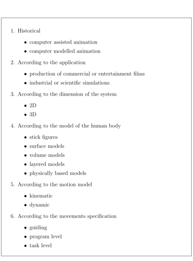
In this chapter, human body animation is examined in detail, under the topics of classification by the application domain, the modeling of human body and the motion model. A classification of human body animation systems can be seen in Figure 2.1. This classification is an extended version of the one given in [30]. We added two subtopics under the model of the human body; layered

models and physically-based models.

2.1 Classification by Application Domain

According to application, human animation is divided into two sections:

pro-duction of commercial or entertainment films, and industrial or scientific sim-ulations.

2.1.1 Production of Commercial or Entertainment Films

The first computer-animated film to win an Oscar is the Tin Toy, a Lasseter film for Pixar. The film was designed by using a key-frame animation system, the film also required extensive facial animation. Skin deformations of the human baby in the film was successful. Another film of Lasseter for Pixar is Luxo Jr., in which a Luxo Lamp character is animated as an articulated

(17)

CHAPTER 2. BACKGROUND AND RELATED WORK 4

1. Historical

• computer assisted animation • computer modelled animation

2. According to the application

• production of commercial or entertainment films • industrial or scientific simulations

3. According to the dimension of the system

• 2D • 3D

4. According to the model of the human body

• stick figures • surface models • volume models • layered models

• physically based models

5. According to the motion model

• kinematic • dynamic

6. According to the movements specification

• guiding • program level • task level

(18)

figure. An example of a realistic human animation film of an existing or existed character is, Rendezvous a Montr´eal by Mira Laboratory [17, 18].

2.1.2 Industrial or Scientific Simulations

Simulations are heavily used in medical, robotics, choreography, ergonomics, aeronautic and automobile engineering and in fashion.

For medical 3D models, medical surgery, virtual cadaver and in many med-ical sciences there exists a growing need for human animation. The Visible

Human Project initiated in 1995 by the U.S. National Library of Medicine, has

been recently completed [26]. A 3D virtual cadaver is a useful data that can be used to investigate and observe the human body. Examples of visualization programs developed for The Visible Human are discussed in [25, 29]. Simu-lation of ballets with the computer is explained in [22] and Life Forms is a project to develop computer-based tools to assist choreographers in composing dance [5]. As an example for the ergonomics, a human model Jack operat-ing a helicopter can be seen in [39]. Fetter’s models were used for operatoperat-ing an aircraft, sitting in automobiles and riding an escalator to a monorail sta-tion [9]. Virtual fashion shows are not common today but it seems in the future there will be many virtual fashion model, showing the virtual versions of real dresses [38, 32].

2.2 Classification by Modeling of Human Body

For human animation, we need to have a model that has a skeleton with joints in order to compute the movements, a skin for human appearance, and the necessary clothing. With respect to the model of human body, human ani-mation can be divided into four groups: stick figures, surface models, volume

models, layered models. Furthermore, some deformation techniques that can

(19)

2.2.1 Stick Figures

A stick figure consists of hierarchical set of rigid segments connected at joints. These models are also called articulated figures. Varying according to the num-ber of segments and joints, stick figure models may be more or less complex. This model can be represented by a tree structure where the nodes point to segments and arcs point to joints. The main advantage of the stick figure is that, the control of the movement is very easy. Representation by a three dimensional matrix for each joint corresponding to its three DOFS would be very easy. The main disadvantage of this model is producing unrealistic vi-sualizations. Without volume perception of the depth, it can not be sensed. Examples for stick model are studies on goal directed motions of articulated figures by Korein et al. [13] and a stick figure by Thalmanns [16].

2.2.2 Surface Models

Surface model consists of a skeleton and a skin as an envelope outside of it. Surface models are examined under four topics: points and lines, polygons, and

curved surface patches and other deformation techniques related to surface

models.

• Points and Lines: A collection of 3D points or lines is the simplest surface

model. For accurate modelling surfaces represented by points require a fairly dense distribution of points . Clouds of points with depth shading were used until the early 1980’s for human models on vector graphics dis-plays. Using parallel rings or strip of points to retain display speed while offering more shape information is a technique used in Life Forms [5].

• Polygons: In polygonal object representation, vertices form polygons,

polygons form surfaces and surfaces form objects. Polygon models are relatively simple to define, manipulate, and display. Many workstation hardware and commercial graphics software use this model in render-ing. In [2], the advantages and disadvantages of the model are stated. The advantages are: modelling objects using polygons is straightforward,

(20)

piecewise linearities in the polygonal structure are rendered invisible by the shading technique, geometric information is only stored at the poly-gon vertices and information required for the reflection model that eval-uates a shade at each pixel is interpolated from this vertex information. The disadvantages are: mapping textures from a two-dimensional do-main onto the surface of an object is difficult, shadow algorithms that are based on polygonal objects generally have high coding complexity and produce hard-edged shadows, polygons are expensive. Films such as

Tony de Peltrie [8] and Rendezvous a Montr´eal [17, 18] are good examples

of this category.

• Curved Surface Patches: Polygons are good at building blocks, so

consid-erable effort has been expended determining mathematical formulations for true curved surfaces. Nets of patches are used to model free form surfaces. Most curved surface object models are formed by one or more parametric functions of two variables (bivariate functions). Each curved surface is called a patch; patches may be joined along their boundary edges into more complex surfaces. There are numerous formulations of curved surfaces, including: B´ezier, Hermite, bi-cubic, B-spline, Beta-spline [3].

2.2.3 Human Body Modeling using Deformation

Tech-niques

If the animation is not physical and there is no contact between the hu-man being and the environment then joint-dependent local deformation (JLD) approach is convenient [19]. This approach is used to improve the realism of motion from the view of deformations of human bodies during animation. In JLD, a flesh (considered as the actor surface) is digitized from a sculpture. Each vertex of this flesh is assigned to a specific point on the skeleton. The deformation is done by JLD operators which are specific local deformation operators depending on the nature of the joints. Each JLD operator is responsible for some uniquely defined part of the surface. This part is called the domain of the operator. Deformation is

(21)

done by the values of the operator which is determined by a function of the angular values of the specific joint angles defining the operator. Another approach to model smoothly blended, plasticine objects is

blob-bies. Also called metaballs or soft objects, their most attractive

fea-ture is their deformability. The shape of the object can be changed by joint movements. By anchoring multiple soft object control points to the skeleton and adjusting their strength appropriately, a blobbie cover-ing the skeleton, can be created. This model will deform smoothly and automatically according to movements of joints [37].

2.2.4 Volume and Constructive Solid Geometry Models

These models divide the world into three-dimensional chunks. For practical applications in need of quick inside outside tests, they seem to be the most ap-propriate application for collision detections or choreography. However, when realism is the major requirement they cannot compete with surface models. Some models such as volume elements (voxels) or oct-trees, are formed from non-intersecting element, while some models called Constructive Solid Geom-etry (CSG) are created by combining the volumes occupied by overlapping three-dimensional objects using set operations. Single primitive systems use the advantage of only using one primitive model, so manipulation and display of the models take less time.

• Voxels: Voxels are tessellation of cubes or parallelopipeds. In this model

space is completely filled with voxels. An octree encoding scheme divides regions of three dimensional space into octants and stores eight data ele-ments in each node of the tree. Here, the root of the octree refers to the entire volume. Voxel models are the basis for many of the scientific visual-ization work in biomedical imaging. The possible detail for human models is only limited by the resolution of the sensor. Accurate bone joint shapes may be visualized, as well as the details of internal and external physio-logical features. These methods have not yet found direct application in the human factors domain, since bio-mechanical rather than anatomical issues are usually addressed [3]. Octrees are particularly appropriate

(22)

for representing sample data volumes common to scientific visualization, where the data points often define a spatial decomposition into hexa-hedral, space-filling, non-overlapping regions. A special type of octrees representing volumes whose resolutions are not conveniently a power of two are called branch-on-need octrees (BONOs). They can be examined in [35]. For marching cubes algorithm, [15] can be referred. Here, marching cubes algorithm is used to process three-dimensional data.

• CSG: Unlike voxel models, for CSG models there is no requirement to

regularly tessellate the entire space. Another difference is in the primitive objects. In voxel model, this is the cube but in CSG this may also be cylinder, sphere, cone, half-space, blocks, pyramids. Here, each primitive can be constructed by a CSG module. To create a new 3D shape, we first select two primitives and drag them into position in some region of space. Then set operations are are applied to create complex models. The object formed with this procedure is represented by a binary tree [11].

• Single Primitive System: The model uses only one primitive instead of

more than one as in CSG. So, only one type of procedure is used to render primitives. Except union operation, other set operations are discarded. Ellipsoids, cylinders, spheres are all basic primitives used in early times to represent human figures. Besides, there is a very special primitive called superquadric. This one is interesting because it has both implicit and parametric representation. Superquadrics were developed by Alan Barr [4] and they have diffirent primitives such as superellipses, superhy-perboloids of one sheet, superhysuperhy-perboloids of two sheets and supertoroid. In this group, mainly the superellipses are most useful primitives.

2.2.5 Layered Models

In layered models, Free Form Deformation (FFD) is one of the techniques used to control the deformation across joints. FFD method is introduced by Sederberg and Parry [24]. Their technique defines a free-form deformation of space by specifying a trivariate B´ezier solid, which acts on a parallelpiped region

(23)

of space. The deformation of the object is accomplished by deforming the objects coordinate system in the following three steps. First, the object to be deformed is embedded in a regular coordinate system defined by three mutually perpendicular axes. Then, the coordinate system is deformed, allowing its previously straight axes to become curves. Afterwards, the positions of the objects vertices in the old (regular) coordinate system are updated to match where they ended up after the coordinate system was deformed.

This method is useful in some cases but it has two main problems: the first problem is that it is hard to predict or control the deformation in the region where FFD blocks intersect and the second one is, it does not synchronize with the underlying articulated figure in a good manner [2]. These problems are attacked by Chadwick et al. [6]. In their system Critter, Chadwick defines layers as a conceptual simulation model that maps higher level parametric inputs into lower level outputs. His body model is composed of four layers from high to low level:

1. Motion specification (behavior layer). 2. Articulated figure (skeletal layer).

3. Muscle and fatty tissue layer (muscles are modelled using FFDs that attached to the skeletal structure).

4. Surface description, surface appearance and geometry (skin clothing and fur layer; in this layer there exists a polygonal skin that acts according to the muscle layer).

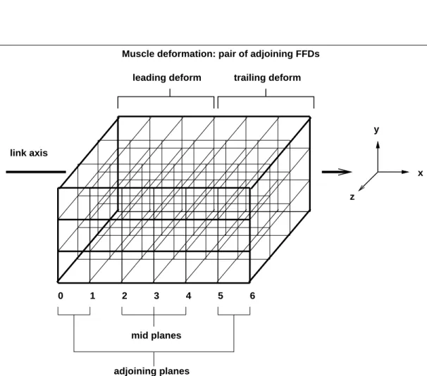
In Critter system various constraint relationships can be defined by the ani-mator and global motion can be controlled from a high level. Muscle and fat deformations are based on FFDs. Muscles are represented by a pair of con-nected hyperpatches (see Figure 2.2). There are four planes for each FFD, with one common plane as the adjoining connection between deformations. So there are seven planes of control points orthogonal to the adjoining connection between deformations. Adjoining planes preserve the continuity while the mid-point planes function to model the muscle behavior according to kinematic or dynamic attribute of the skeleton layer.

(24)

CHAPTER 2. BACKGROUND AND RELATED WORK 11 0 1 2 3 4 5 6 mid planes adjoining planes link axis z y x leading deform trailing deform

Muscle deformation: pair of adjoining FFDs

Figure 2.2: Muscle primitive as a pair of adjoining FFDs [Courtesy of J.E. Chadwick, D.R. Haumann and R.E. Parent. Layered Construction for De-formable Animated Characters. ACM Computer Graphics (Proc. of

(25)

2.2.6 Physically Based Models

To improve animation, industry requires more realistic models. Physically based modelling uses dynamic motion model, so it can give great realism and these active models can react automatically to internal and external environ-mental constraints such as fields, collisions, forces, torques, velocities, accelera-tions, heat. However, they have also disadvantages stated in Subsection 2.3.2. Physically based modelling can be grouped as: rigid objects model, deformable

objects model, particle model and mass-spring model.

• Rigid Objects Model: When deformable and particle models approach to

inflexibility they are called rigid bodies. It is commonly used in robotics, engineering, physics etc. There are many studies on the subject. One of them is about dynamics of articulated rigid bodies by Armstrong et al. [1].

• Deformable Objects Model: These models are based on continuum

me-chanics [31]. Continuum meme-chanics includes elastic, deformable and fluid materials. Deformable models based on elasticity theory are developed by Terzopoulos et al. [27]. Besides, hybrid model containing rigid body and elastic components are studied by Terzopoulos and Witkin [28]. For the ones about human body deformations, [10] can be referred.

• Particle Model: To simulate definite events in nature such as water,

smoke, and fire this model is used. Particle model is developed from single particle dynamics. Examples are, water by Kass et al. [12], smoke by [7] and, the fire effects by Loke et al. [14].

• Mass-spring Model: Mass-spring model is useful for modelling reasonably

flexible types of material such as jello and elastic surfaces. In this model to simulate the muscles, Nedel [21] used a mass-spring system, in which a new kind of springs called angular springs are used. They are formed to control the muscle volume during simulation. In order to mechani-cally quantify the force produced by a muscle over a bone muscles are represented by lines, called action lines.

(26)

2.3 Classification by Motion Model

With respect to the motion model, human motion is covered under two topics:

kinematic models and dynamic models.

2.3.1 Kinematic Models

Kinematic models study motion independent of the underlying forces that pro-duced the motion. It is the relationship between the positions, velocities, and accelerations of the links of a manipulator, where the manipulator is an ex-tremity of the human body such as hand or foot. It is divided into two:

• Forward Kinematics: computation of the position, orientation and

veloc-ity of the end effector, given the displacements and joint angles.

• Inverse Kinematics: computation of the joint displacements and angles

from the end effectors position and velocity.

2.3.2 Dynamic Models

Dynamic models respond to gravity and inertia. Motion is computed under the effect of the forces, the torques, the constraints and the mass properties of objects. There are some advantages and disadvantages of dynamic simulations. The advantages are: reality of natural phenomena is better rendered, dynamics frees the animator from having to describe the motion in terms of the physical properties of the solid objects, bodies can react automatically to internal and external environmental constraints: fields, collisions, forces and torques. The disadvantages are: systems are hard for the animator to control, parameters (e.g. forces or torques) are sometimes very difficult to adjust, amount of CPU time required to solve the motion equations of a complex articulated body using numerical methods is high, they are too regular, because they do not take into account the personality of the characters. Dynamic models are also divided into two: forward dynamics and inverse dynamics.

(27)

• Forward Dynamics: finding the trajectories of some point (e.g., an end

effector in an articulated figure) according to the forces and torques that cause the motion.

• Inverse Dynamics: determine the forces and torques required to produce

(28)

Chapter 3 Human Figure Modelling

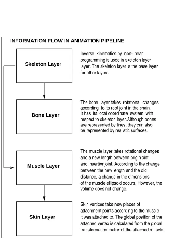
In this chapter, we mention about our animation system in general. The mod-eling system used is a layered one. It is a hybrid model composed of four layers that are skeleton layer, bone layer, muscle layer and skin layer. The best property of a hybrid layered approach is that a different and appropriate method can be used at different layers according to their special features. Fa-cial and hand animations are not considered. Explanation is done from inner to outer layers. Skeleton layer, which uses inverse kinematics by non-linear programming for motion control, is a base frame for other layers. Bone layer is represented by lines. In muscle layer, muscle representation with ellipsoids and muscle modification are explained. In skin layer, skin attaching and skin deformation are described. The diagram for layered animation flow can be seen in Figure 3.1.

3.1 Motion Control at the Skeletal Layer

An articulated figure is a structure that consists of a series of rigid links con-nected at joints and the number of DOF of an articulated figure is the number of independent position variables necessary to specify the state of a structure. The end-effector is the free end of a chain of links [2]. The aim in the animation is to move the end-effector towards a goal.

(29)

CHAPTER 3. HUMAN FIGURE MODELLING 16

INFORMATION FLOW IN ANIMATION PIPELINE

be represented by realistic surfaces. are represented by lines, they can also according to its root joint in the chain. respect to skeleton layer.Although bones programming is used in skeleton layer for other layers.

It has its local coordinate system with

attachment points according to the muscle Inverse kinematics by non-linear

Bone Layer

Muscle Layer

Skin Layer

The bone layer takes rotational changes layer. The skeleton layer is the base layer

it was attached to. The global position of the attached vertex is calculated from the global transformation matrix of the attached muscle.

Skeleton Layer

The muscle layer takes rotational changes and insertionjoint. According to the change between the new length and the old of the muscle ellipsoid occurs. However, the volume does not change.

and a new length between originjoint distance, a change in the dimensions

Skin vertices take new places of

(30)

struct joint { char *name;

Site *site1, *site2; Joint *rootjoint; DOF *dofs; int ndofs; Vector displacement; Matrix global; JointGroup *joint_group_it_belongs; int index_in_JointGroup; }

Figure 3.2: Joint data structure

If all the joint angles are known and we are searching for a coordinate, the motion of the end effector is determined indirectly from all transformations to the end effector. This is called forward kinematics. If we know the position of the end-effector and the goal, and if by means of these inputs, position and orientation of all joints in the link hierarchy are solved, this is called inverse

kinematics. In a real skeleton there are many joints. Of course modelling

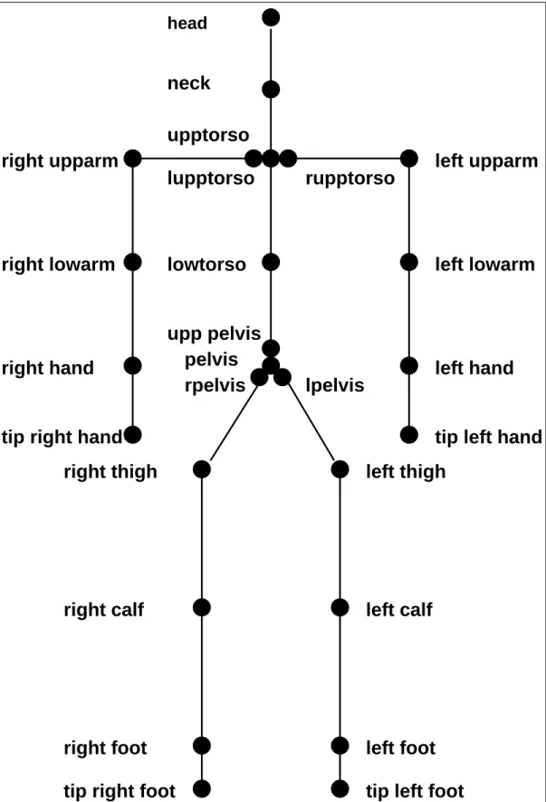
each joint would be very complex and not time efficient. So, in our animation model, the model is simplified. To move all these simplified joints is a difficult act, which falls under the category of articulated figure animation. Instead of using real skeleton data, stick representation is used for computational speed. The articulated figure is moved to desired position by inverse kinematics using nonlinear programming. The goal is selected by the user interactively [40]. To express the situation clearly, we better take a look at the joint data structure in Figure 3.2. Joint structure of our human model is given in Figure 3.3. In a figure each joint has three rotational and three translational DOFs. However, in human animation translational DOFs can be neglected so we did not use translational DOFs. As it can be seen from Figure 3.2, each joint has a group. When we choose an end-effector and try to reach a goal, all joints in that end-effector’s chain are affected by this motion. One end of this chain does not move at all, but the other end which is called end effector is free to move. There is a transformation matrix M between two coordinate frames in the chain sharing the same point. The transformation matrix Mi at a rotation joint i, is

(31)

neck

upptorso

upp pelvis

left thigh

left calf

rpelvis

lupptorso

head

rupptorso

left foot

tip left foot

tip left hand

left hand

left upparm

lowtorso

lpelvis

left lowarm

pelvis

tip right hand

right hand

right lowarm

right upparm

right thigh

right calf

right foot

tip right foot

(32)

a concatenation of a translation and a rotation. These are done according to parent joint of joint i.

Mi = T (xi, yi, zi)R(θi) (3.1)

Here, T(xi, yi, zi) is the translation matrix that translates the joint i from its

root joint i-1 and R(θi) is the orientation matrix that rotates joint i’s rotation

axis by θi. The composite matrix between any two coordinate systems i and j

in the joint chain is found by concatenating the transformations at the joints from joint i to joint j [33].

Mij = MiMi+1...Mj−1Mj (3.2)

The position and orientation of the end-effector with respect to root are found by concatenating the transformations at each joint in the chain.

3.2 Bone Layer

Bones are rigid bodies forming the skeleton. They are connected to each other by joints. There are 206 bones in human body [20]. In this layer, lines are used to represent the bones. Each bone has a local coordinate system attached to the rootjoint of its structure. The world coordinates of bones are calculated with respect to their rootjoint. Instead of using lines, real skeleton data can be used but this model will make a decreasing effect on CPU time and refresh rate accordingly.

3.3 Muscle Layer

3.3.1 Muscle Representation

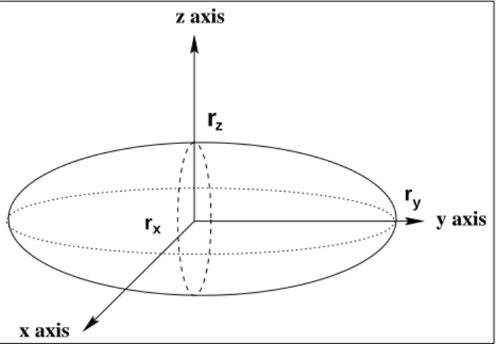
Ellipsoids are basic structures for our representation. An ellipsoidal surface

can be described as an extension of a spherical surface, where radii in three perpendicular directions can have different values (Figure 3.4). The Cartesian representation for points over the surface of an ellipsoid centered on the origin is shown as,

(33)

CHAPTER 3. HUMAN FIGURE MODELLING 20 x axis y axis z axis rz rx y r

Figure 3.4: An ellipsoid with radii rx, ry, rz centered on the coordinate origin.

(x rx )2_{+ (} y ry )2_{+ (}z rz )2 _{= 1} _(3.3) x = rxcos Φ cos Θ, − Π 2 ≤ Φ ≤ Π 2, (3.4) y = rycos Φ sin Θ, −Π ≤ Θ ≤ Π, (3.5) z = rzsin Φ (3.6)

Ellipsoid is used to model muscles, because they allow faster inside/outside tests. If this test is tried for a particular voxel with points (x,y,z), it can be seen that, voxel is inside when f(x,y,z) < 0, outside when f(x,y,z) > 0 and on the surface when f(x,y,z) = 0. Ellipsoids are placed on their local coordinate frames. Their world coordinate frames are calculated by their global matrices (see Figure 3.6) for speed. Ellipsoid’s volume can be calculated as in Equation 3.7 and stored in musclevol (Figure 3.6). Ellipsoid’s volume does not change during animation. In order to keep the volume constant, both the volume and the r value (rx

ry), is stored before motion, while the body is in rest state. As the muscle volume change, the z, y, x values change in order according to r. The volume of an ellipsoid is given by Equation 3.7.

υ = 4πrxryrz

3 . (3.7)

3.3.2 Muscle Data Structure

Muscles are deformable bodies attached to bones with tendons. Muscles, ten-dons and bones are all covered with fatty layer. This fatty layer has skin around

(34)

class dimension { public:

float x; //x, y, z radii of the

float y; ellipsoid.

float z;

float scalex; //scaling factors for

float scaley; x, y, and z radii.

float scalez; };

Figure 3.5: Ellipsoid dimensions data structure

it. In this thesis only muscles and skin are simulated. Bones are represented by lines and fatty layer is the distance between the attachment point and the skin point. Muscle structure is inside segment structure, and via segment’s joint structure muscles are attached as links to the skeleton joints so that they move as components of an articulated figure. There are three kinds of muscles according to their position in the body and to the characteristic of their fibres;

skeleton muscles, straight muscles and heart muscles. Only skeleton muscles

are examined here. Approximately there are 600 muscles in a human body. When a muscle bulges, it thickens and shortens. So, an ellipsoid structure fits nicely to muscle structure. A bulged muscle is restored to its original position by its contrary muscle. However, in our simulation model it is restored by the movements of the articulated figure.

Muscles are under the skin layer. They are simplified versions of real mus-cles simulated by ellipsoids. In reality, force that gives motion to bones, is activated by muscles as nerves trigger muscles by the signals coming from the brain. Here this is not the case. Muscles are activated by the movement of bones where they are attached. In our system this attachment is a virtual one. Tendons are not drawn. First attachment point that is closer to the root of the tree structure is called the originjoint and the second attachment point farther from the root in the tree structure is called insertionjoint. The length between these two points is calculated and according to the change in the length value, the dimensions of the muscle are changed.

(35)

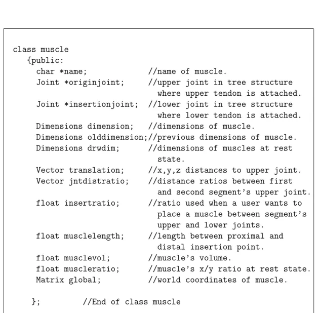
class muscle {public:

char *name; //name of muscle.

Joint *originjoint; //upper joint in tree structure

where upper tendon is attached. Joint *insertionjoint; //lower joint in tree structure

where lower tendon is attached. Dimensions dimension; //dimensions of muscle.

Dimensions olddimension;//previous dimensions of muscle.

Dimensions drwdim; //dimensions of muscles at rest

state.

Vector translation; //x,y,z distances to upper joint.

Vector jntdistratio; //distance ratios between first

and second segment’s upper joint.

float insertratio; //ratio used when a user wants to

place a muscle between segment’s upper and lower joints.

float musclelength; //length between proximal and

distal insertion point.

float musclevol; //muscle’s volume.

float muscleratio; //muscle’s x/y ratio at rest state.

Matrix global; //world coordinates of muscle.

}; //End of class muscle

(36)

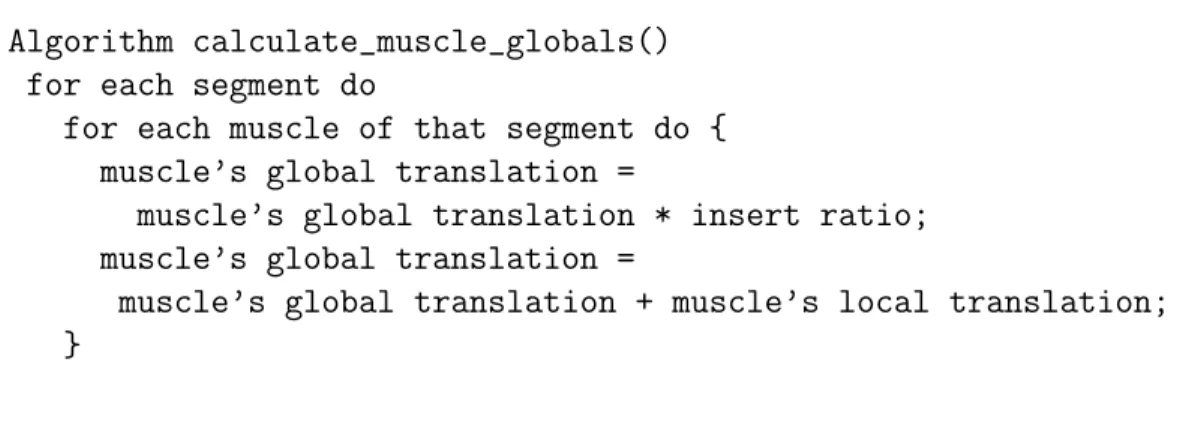
Algorithm calculate_muscle_globals() for each segment do

for each muscle of that segment do { muscle’s global translation =

muscle’s global translation * insert ratio; muscle’s global translation =

muscle’s global translation + muscle’s local translation; }

Figure 3.7: The algorithm for calculating the global coordinates of the muscle

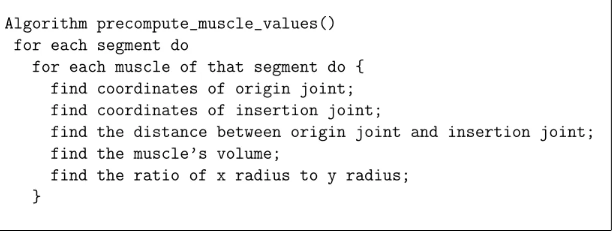
Muscles can be placed anywhere according to the root joint of its segment. Different bulging shapes can be obtained by changing the placement of origin and the insertion joints (see Figure 3.6). By means of two distance ratios from upper and lower joints, the coordinates of segment’s origin joint and insertion joint can be changed. The ratio of change would be big if the length between these two points is short and ratio of change would be small if the length between these insertion points is long. Figure 3.9 illustrates the situation. Before the precomputation for each muscle, global coordinates of each muscle is found as shown in the algorithm in Figure 3.7. After finding each muscle’s global, a precomputation is made for all muscles. In this precomputation each muscle’s, length between the origin point and the insertion point, volume, rx

ry (the length of x axis over the length of y axis) is found and stored for future use. The algorithm for calculating the global coordinates of a muscle is given in Figure 3.8.

3.3.3 Muscle Deformation

Muscle layer is modelled by 75 ellipsoidal muscles. So we can say, single

prim-itive systems are used to model muscles. As it was stated in section 2.2.4,

single primitive system uses the advantage of only using one primitive model, so manipulation and display of the models take less time. For the deformation of muscles kinematic deformation is applied. This technique changes the x, y, z

(37)

Algorithm precompute_muscle_values() for each segment do

for each muscle of that segment do { find coordinates of origin joint; find coordinates of insertion joint;

find the distance between origin joint and insertion joint; find the muscle’s volume;

find the ratio of x radius to y radius; }

Figure 3.8: The algorithm for muscle values.

radii of the muscle according to the change between origin point and insertion point. Let us call the new distance between these points as new length (lnew),

the beginning distance between these points the entry length (lentry), volume

υ, the x, y, z axis lengths of the muscle at the beginning state (rx, ry, rz) and

constant ratio const which equals to (rx

ry). When a motion is detected and if that muscle does belong to a segment which has a joint on that moving chain then radii of the muscle are adjusted according to the Equations 3.8, 3.9, and 3.10. rznew = c lnew lentry , (3.8) r_ynew = s 3υ 4rz new(const)Π , and (3.9)

rxnew= r_ynew(const). (3.10)

The volume of the muscle is conserved during this operation. When a motion is detected, the shape of the muscles change with respect to the change between (lnew) and (lentry). If lnew < lentry, muscle bulges else the muscle turns into a

thinner shape. After computation is completed, muscle must be carried to its new position in space. To carry it to its new position, first it is rotated by the amount of its origin joint’s rotation and translated by an amount of its origin joint’s translation plus muscle’s translation. The algorithm for muscle deformation is presented in Figure 3.10.

(38)

CHAPTER 3. HUMAN FIGURE MODELLING 25 10 cm 10 cm 10 cm 10 cm 10 cm 5 cm 5 cm 10 cm 20 cm 15 cm 14.1421cm 11.18 cm 14.1421 20 11.18 15 ratio = --ratio = ---ratio = 0.7071 ratio = 0.7453 originpoint originpoint originpoint insertionpoint originpoint insertionpoint insertionpoint insertionpoint

Figure 3.9: Muscle deformation. The deformation ratio would be large, if the length between origin point and insertion point is short, and muscle deforma-tion ratio would be small if the length between these points is long.

(39)

Algorithm update_muscles(Jointgroup chain) for each segment do {

if (segment’s ujoint and ljoint in chain) for each muscle of that segment do {

copy segment’s ujoint’s global translation to vector1; copy segment’s ljoint’s global translation to vector2; copy segment’s lsegment’s ljoint’s

global translation to vector3; vector4 = vector2 - vector1;

vector5 = vector3 - vector2; first point = vector2 +

(vector4 * origin joint’s placement ratio); second point = vector3 +

(vector5 * insertion joints’s placement ratio); vector between points = first point - second point;

}

new distance =

sqrt(vector between points . vector_between_points); muscle’s old z radius = muscle’s z radius;

muscle’s z radius = muscle’s z radius *

(new distance / old distance); muscle’s y radius = muscle’s y radius;

muscle’s y radius =

sqrt(3 * segment’s muscle volume /4 * muscle’s z radius * (x radius/ y radius at rest state) * Pi);

muscle’s old x radius = muscle’s x radius; muscle’s x radius = muscle’s y radius *

(muscle’s x radius / y radius at rest state); }

(40)

class vertex { public:

Segment *vertexseg; //pointer to nearest segment

int musclenum; //number of muscles in the segment

int musclevertexnum; point globalpoint; pointint localpoint;

float global[3]; //global coordinates of vertex

float local[3]; //local coordinates of muscle

float attachment[3]; //length to surface point from center of muscle

float surface[3]; //length to skin vertex point

from surface attachment point. }; //end of class vertex

Figure 3.11: Vertex data structure

3.4 Skin Layer

Skin is an organ that covers the whole body, and protects the organism from the harmful effects of the outer environment. Our goal in skin layer is to deform it according to muscle deformations. So, by this way, improve the realism of skin surface. segment structure simulates the skin and it is drawn by a group of triangles.

3.4.1 Skin Data Structure

The data structure of the segment is shown in Figure 3.12. The data of our skin is taken from a VRML avatar data. A VRML avatar file has vertex coordinates and also indices to these coordinates, as shown in Figure 3.13. Muscles must be positioned appropriately so that they cannot be seen when covered with the skin. After that, the skin must be attached to the nearest muscle. Before attaching, each skin point must be represented in the local coordinate system of the current ellipsoid that it is tested with and the nearest point on one of the ellipsoids is found. In our solution skin vertices are placed according to their segment’s local coordinates, so the segment it belongs to, the upper and the

(41)

class segment { public:

char *name; char *fullname;

Joint *upperjoint; //joint close to root joint

Joint *lowerjoint; //joint far from root joint

Segment *uppersegment;//segment closer to root joint Segment *lowersegment;//segment far from root joint

char *filenamev; //file containing indexes to edges

char *filenamef; //file containing indexes to nodes

int totmusclenum; //total number of muscles

Muscle muscles[12]; //muscles in segment

int precomputed; //whether a precompute is needed

point pointvect[1000]; vertex vertex[2000]; float normal[1000][3];

float color[3]; //three color values for rendering

int nedges; //total number of edges

int nnodes; //total number of nodes

};//End of class segment

Figure 3.12: Segment data structure

2.333 1.899 3.455 1.785 2.222 8.147 2.769 3.276 1.428 5.676 4.594 7.878 8.543 2.876 3.432 3.123 2.345 5.434 X Y Z 0 1 2 0 1 5 1 3 4 2 1 5 5 4 3

(42)

lower segment, are examined for the nearest muscle. Totally three segments’ muscles are examined for this purpose.

3.4.2 Attaching the Skin

To attach the skin vertices, the method described in [34] is used. If we solve the ellipsoid equation for a certain point, this does not give us the distance to the nearest point on the ellipsoid. For that reason, an iterative Newton

Raphson method is used. Taking the derivative of the ellipsoid equation at

the nearest point on the ellipsoid to the skin point, we get a vector between the point and its nearest point. A parametric line equation representing that vector is found. When parameter t = 0, we are at the skin point, and taking small steps along the line dt brings us toward the nearest point. There is also another parameter, called g(t), which is the ellipsoid equation parameterized by t. Let (xs, ys, zs) be the skin point in the ellipsoid coordinate frame and

(a,b,c) be the ellipsoid axis lengths. The parameter t is initialized to zero and

dt is initialized to a small fraction of the value of f(0). The iteration continues

until the absolute value of dt is acceptably small or the number of iterations reaches a prespecified value.

x = xs∗ a2 (a2_{+ 2t)} (3.11) y = ys∗ b2 (b2_{+ 2t)} (3.12) z = zs∗ c2 (c2_{+ 2t)} (3.13) g(t) = a2x2s (a2_{+ 2t)}2 + b2_y2 s (b2_{+ 2t)}2 + c2_z2 s (c2 _{+ 2t)}2 (3.14) g0(t) = −4a 2_x2 s (a2_{+ 2t)}3 + b2_y2 s (b2_{+ 2t)}3 + c2_z2 s (c2_{+ 2t)}3 (3.15) dt = −1.0 ∗ (g(t) − 1) g0_(t) (3.16) t = t + dt (3.17)

(43)

y-axis

z-axis

skin

point

center of the muscle

to skin point

total distance from

x-axis

remaining

distance

point

distance

attachment

(44)

output of this iteration, and this voxel is called the attachment point. The attachment point is the vertex from the center of the ellipsoid to the nearest point on the ellipsoid. The remaining vertex is from the nearest point to the skin point, and it is called surface point (see Figure 3.11). To express it clearly, let us think of a sphere surrounded by a cube. Thus, we can think that our muscle has a skin that has eight vertices. Let the radius of the sphere be one unit and side of the cube be two units. After the computation is completed, the length between the center of the muscle and the attachment point will all be 1 unit and the length between the attachment point and the skin vertex will be equal to √3 − 1. In Figure 3.14, the first distance is named as attachment distance and the second distance is named as surface distance. As it was mentioned above, the algorithm returns us the nearest point on the ellipsoid. When we subtract these values from the local skin coordinates of that point, we get three values that are x, y, z values for surface point. (xskin− xattachment, yskin − yattachment, zskin− zattachment). So, the local

coordinates of attachment point are ( ±_√1 3, ± 1 √ 3, ± 1 √

3). The sign of the values

differs according to the corner of the cube checked. We know the local x, y, z coordinates of the skin that are (±1, ±1, ±1), so surface point can be found from these values. Attaching is done once at the beginning of the computation as a precomputing operation. The attaching algorithm is as in Figure 3.15.

3.4.3 Skin Deformation

Our goal in the skin layer is to simulate skin deformations caused by joint and muscle deformations. Whenever a movement is detected, new positions of at-tachment points must be recalculated. As skin points move with respect to the skin muscles, their new values are calculated from the ratio of new dimensions and old dimensions. So, new values are calculated for each dimension of the muscles of the corresponding segment. Here the important point is that this is not done for surface vertex since its dimension values do not change according to muscle dimension variations (Figure 3.17). Since skin vertex values are de-termined with respect to muscle vertex values they are attached to, they inherit rotation and translation from the muscle they were anchored. The algorithm to calculate the global for each vertex can be seen in Figure 3.16.

(45)

Algorithm attaching_skin()

initialize t to 0 and distance to a big number for each segment do

for each muscle of current segment, upper and

lower segment of that segment do { find global coordinates of skin vertex

calculate local coordinates of skin vertex according to that muscle

With local coordinates of skin vertex and x, y, z radii of that muscle

for j = 1 to 10 do

do the Newton Raphson iteration using local coordinates of skin vertex and x, y, z radii of current muscle //Section 3.4

temp = newlength

if (distance > newlength) then { distance = temp

attachment[0] = x value calculated by the iteration attachment[1] = y value calculated by the iteration attachment[2] = z value calculated by the iteration

surface[0] = local x value of skin vertex - attachment[0] surface[1] = local y value of skin vertex - attachment[1] surface[2] = local z value of skin vertex - attachment[2] vertexseg = address of segment in current iteration

musclenum = current muscle number in that segment }

}

(46)

Algorithm calculate_vertex_global_coords() for each segment do

for vertex of that segment do {

copy identity_matrix to translation_matrix; for j = 1 to 3 do

translation_matrix[3][j] = attachment[j] + surface[j]; result_matrix = (translation_matrix *

muscle’s_global_transformation_matrix); for j=1 to 3 do

current_vertex[j] = result_matrix[3][j]; }

Figure 3.16: The algorithm for calculating the new global coordinates of the vertices

Here the crucial point is that if our model does not have enough vertices, deformations at joints would not be so proper. So, especially skin surface near the joints must be drawn with dense triangulation. Besides, locating muscle bellies near the joints that have low bulging property would prevent improper deformations. Once muscles are placed under the skin, they do not need to be drawn.

(47)

Muscle

Skin

Muscle

attachment vector surface vector surface vector attachment vector attachment vector surface vector attachment vector surface vector skin point skin point

(a)

(b)

Figure 3.17: Comparison of attachment and surface vectors: (a) neutral state, and (b) after muscle bulging.

(48)

Chapter 4 Implementation Details

In this section, the implementation details of the system and the test results obtained by using the system are explained.

4.1 Implementation

Our human model is composed of 18 bones, 75 muscles and 1,797 triangles for segment drawings. Bones are simulated with lines, so they do not have an important contribution on total performance. The tests for the implementation was made on a personal computer with Celeron (TM)-MMX1_{–400MHz CPU,}

having 64 MB of main memory. The animation system is implemented by using C++ language and OpenGL2_{. For developing the user interface, GLUI}

library is used.

4.2 Performance Experiments

In this section we discuss the performance experiments and present the results of our system. It was stated that deformations at skin must be dense to observe

1_{Celeron is a registered trademark of Intel Corporation.} 2_{OpenGL is a registered trademark of Silicon Graphics, Inc.}

(49)

CHAPTER 4. IMPLEMENTATION DETAILS 36

deformation at joints. So, we examine deformations of the skin with respect to bulging of muscles and deformations at joints, on the dense triangulated left leg figure.

The average frame rates for different layers are given in Table 4.1. In the table, both single and composite layer performance results are given. As it can be seen from the table, bone layer does not have a considerable effect on the performance. We draw muscles by OpenGL functions.

In order to shorten rendering time, we preferred to use constant shading since constant shading makes intensity calculations very fast [11]. Although constant shading does not provide smooth appearance as its counterparts like Gouraud shading, when the number of vertices is quite enough this disadvan-tage does not cause any visual artifact.

Table 4.1: Average frame rates for different layers.

Active Layer(s) Shaded Not Shaded

Bone 31.4 32.4

Muscle 0.9 2.8

Skin 14.6 19.3

Muscle and skin 0.8 2.6

Muscle and bone 0.9 2.8

Skin and bone 14.5 19.3

Muscle, skin and bone 0.8 2.6

4.2.1 Skin Deformations

A dense triangulated right leg is chosen, to show the deformations of the skin after muscles bulge and the deformation at joints. Here the data used belongs to a complete right leg. It is not fragmented into right thigh, right calf and right foot segments. The data of the complete right leg data is used as an right thigh segment data and right calf is not drawn. As attaching algorithm is applied to the vertices, the vertices near the right calf are attached to nearest muscles of right calf. This dense data is composed of 2,519 vertices and 5,028 faces that is three times as big as our whole Juliet data. The skin at the right

(50)

calf joint while in rest state and after deformation can be seen in Figure 4.1.(a) and 4.1.(b), respectively. As it can be seen from Figure 4.2, spheres are used at

(a) (b)

Figure 4.1: (a) skin on right calf at rest state, and (b) deformation of skin at right calf.

joints to get a sufficient deformation at the calf joint. Without these spheres, improper deformations may occur. For a convenient deformation, placing mus-cles inside the skin is important (Figure 4.3.(a)). In order to obtain different muscle bulging, the length from the origin point and the insertion point to their root joints is modified. So, some muscles deform more and some less. The muscles used for proper skin deformations at joints, do not deform at all (Figure 4.3.(b)). Deformation of skin while right calf is rotated 90o _{can be seen}

(51)

Figure 4.2: Four spheres simulating muscles, the upper two muscles are placed with respect to the thigh joint and the lower two are placed with respect to the right calf joint.

(52)

(a) (b)

(c) (d)

Figure 4.3: (a) muscles at rest state, (b) muscle deformation after rotation of right calf, (c)skin at rest state, and (d)deformed skin.

(53)

Chapter 5 Conclusion and Future Work

5.1 Conclusion

In this study, we implemented a human animation system that uses a mus-cle based layered representation for the human figure modelling for realistic rendering.

The first goal of the implementation is to obtain a satisfactory refresh rate. The refresh rate must be 25 fps for a real-time visualization. The refresh rate of the animation system is about 14.65 fps when the human figure is shaded and 19.3 when the human figure is not shaded. Average refresh rate is 16.975 fps. This result is very near to real time.

The second goal of the implementation is to create a realistic human model. The humanoid used in the animation system is realistic but the total number of vertices used is not enough. Besides, the upper leg used in implementation is very realistic with 2,519 vertices and 5,028 faces.

Muscle bulge simulation is the third objective. As it can be seen from Figure 4.1.(b), we succeeded this objective.

Proper deformations of skin at joints is the fourth goal of the implemen-tation. It can be concluded that skin deformations are realistic for rotations

(54)

CHAPTER 5. CONCLUSION AND FUTURE WORK 41

with angles smaller than 90o_{. However, skin deformations at the joints are not}

so realistic for rotations with angles greater than 90o_.

5.2 Future Work

In skeleton layer, instead of kinematic model using dynamic model can be more accurate but it brings more computation cost at the same time. Bone layer can be represented by realistic data so that animator can better concentrate on muscle movements. We have used only ellipsoid structure to model muscles but this model is not appropriate for all muscles like bending muscles. Bending muscles via kinematic calculations can be simulated by cubic B´ezier curves as implemented by Scheepers et al. (For more detail [23] can be referred). The model presented in [23] is also convenient for our implementation because we also use kinematic motion control. Besides, muscles can be represented by deformable cylinders as in [36]. Fat layer, between muscle layer and skin layer, can be convenient to animate external forces. For simulating the fat layer, the unchanging surface vector can be modelled by spring forces. A self-collision detection module is necessary to prevent the body parts from intersecting each other. Besides, a skin generating algorithm module can be created to cover bone, muscle and fat layer by skin.

(55)

Bibliography

[1] W. Armstrong and M. Green. The dynamics of articulated rigid bodies for purposes of animation. The Visual Computer, Vol. 1, No. 4, pp. 231–240, 1985.

[2] M. A.Watt. Advanced Animation and Rendering Techniques. Third Edi-tion, ACM Press, New York, 1994.

[3] N. Badler, C. Phillips, and B. Webber. Simulating Humans: Computer

Graphics, Animation, and Control. Oxford University Press, Oxford, 1999.

[4] A. Barr. Superquadrics and angle-preserving transformations. IEEE

Com-puter Graphics and Applications, Vol. 1, No. 1, pp. 11–23, 1981.

[5] T. Calvert, A. Bruderlin, J. Dill, T. Schiphorst, and C. Welman. Desk-top animation of multiple human figures. IEEE Computer Graphics and

Applications, Vol. 13, No. 3, pp. 18–26, 1993.

[6] J. Chadwick, D. Haumann, and R. Parent. Layered construction for de-formable animated characters. ACM Computer Graphics (Proc. of

SIG-GRAPH’89), Vol. 23, No. 3, pp. 243–252, 1989.

[7] N. Chiba, K. Muraoka, H. Takahashi, and M. Miura. Two-dimensional visual simulation of flames, smoke, and spread of fire. The Journal of

Visualization and Computer Animation, Vol. 5, No. 1, pp. 37–54, 1994.

[8] A. Emmett. Digital portfolio: Tony de peltrie. Computer Graphics World, Vol. 8, No. 10, pp. 72–77, 1985.

(56)

BIBLIOGRAPHY 43

[9] W. Fetter. A progression of human figures simulated by computer graph-ics. IEEE Computer Graphics and Applications, Vol. 2, No. 9, pp. 9–13, 1982.

[10] J. Gourret, N. Magnenat-Thalmann, and D. Thalmann. Simulation of object and human skin deformations in a grasping task. ACM Computer

Graphics (Proc. of SIGGRAPH’89), Vol. 23, No. 3, pp. 21–30, 1989.

[11] D. Hearn and M. P. Baker. Computer Graphics. Second Edition, C Version, Prentice Hall, New Jersey, 1997.

[12] M. Kass and G. Miller. Rapid, stable fluid dynamics for computer graph-ics. ACM Computer Graphics (Proc. of SIGGRAPH’90), Vol. 24, No. 4, pp. 49–57, 1990.

[13] V. Korein and N. Badler. Techniques for generating the goal directed mo-tions of articulated pictures. IEEE Computer Graphics and Applicamo-tions, Vol. 2, No. 9, pp. 71–74, 1982.

[14] T. S. Loke, D. Tan, H. S. Seah, and M. H. Er. Rendering fireworks displays.

IEEE Computer Graphics and Applications, Vol. 12, No. 3, pp. 33–43,

1992.

[15] W. Lorensen and H. Cline. Marhing cubes: A high resolution 3d sur-face construction algorithm. ACM Computer Graphics (Proc. of

SIG-GRAPH’87), Vol. 21, No. 4, pp. 163–169, 1987.

[16] N. Magnenat-Thalmann and D. Thalmann. Computer Animation: theory

and practice. Springer-Verlag, Berlin, 1985.

[17] N. Magnenat-Thalmann and D. Thalmann. Synthetic Actors in 3-D Computer-Generated Films. Springer-Verlag, New York, 1990.

[18] N. Magnenat-Thalmann and D. Thalmann. Complex models for animating synthetic actors. IEEE Computer Graphics and Applications, Vol. 11, No. 5, pp. 32–44, 1991.

[19] N. Magnenat-Thalmann and D. Thalmann. The direction of synthetic actors in the film. Rendez-vous a Montr´eal. IEEE Computer Graphics

(57)

BIBLIOGRAPHY 44

[20] L. Nedel and D. Thalmann. Modeling and deformation of the human body using an anatomically based approach. In Proc. of Computer Animation

(CA’98), pp. 34–40, 1998.

[21] L. Nedel and D. Thalmann. Real time muscle deformations using mass-spring systems. In Proc. of Computer Graphics International (CGI’98), pp. 156–165, 1998.

[22] G. Savage and J. Officer. Choreo an interactive computer model for dance. In Proc. of the Fifth Man-Computer Communications Conference,

Cal-gary, Academic Press Inc, pp. 233–249, 1977.

[23] F. Scheepers, R. Parent, and W.C.S.F. May. Anatomy-based modelling of the human musculature. ACM Computer Graphics (Proc. of

SIG-GRAPH’97), pp. 163–172, 1997.

[24] T. W. Sederberg, S. R. Parent. Free-form deformation of solid geometric models. ACM Computer Graphics (Proc. of SIGGRAPH’86), Vol. 20, No. 4, pp. 151–160, 1986.

[25] D. Sims. Putting the visible human to work. IEEE Computer Graphics

and Applications, Vol. 16, No. 1, pp. 14–15, 1996.

[26] V. Spitzer and D. Whitlock. The visible human project. In

http://wwwcgsb.nlm.nih.gov./apdb/vhmain.html, 1991.

[27] D. Terzopoulos, J. Platt, A. Barr, and K. Fleisher. Elastically deformable models. ACM Computer Graphics (Proc. of SIGGRAPH’87), Vol. 21, No. 4, pp. 205–214, 1987.

[28] D. Terzopoulos and A. Witkin. Physically-based models with rigid and de-formable components. IEEE Computer Graphics and Applications, Vol. 8, No. 6, pp. 41–51, 1988.

[29] U. Tiede, T. Schiemann, and K. Heinz. Visualizing the visible human.

IEEE Computer Graphics and Applications, Vol. 16, No. 1, pp. 7–9, 1996.

[30] D. Tost and X. Pueyo. Human body animation: a survey. the Visual

Realistic rendering of human models

REALISTIC RENDERING OF

HUMAN MODELS

a thesis

submitted to the department of computer

engineering

and the institute of engineering and science

of b˙ilkent university

in partial fulfillment of the requirements

for the degree of

master of science

by

G¨ultekin Arabacı

September, 2001

ABSTRACT

REALISTIC RENDERING OF HUMAN MODELS

¨

OZET

˙INSAN MODELLER˙IN˙IN GERC¸E ˘GE UYGUN

OLARAK G ¨

OR ¨

UNT ¨

ULENMES˙I

T¨

urk Silahlı Kuvvetleri’ne

ve

Aileme.

ACKNOWLEDGMENTS

Contents

List of Figures

List of Tables

List of Symbols and Abbreviations

Chapter 1

Introduction

1.1

Organization of the Thesis

Chapter 2

Background and Related Work

2.1

Classification by Application Domain

2.1.1

Production of Commercial or Entertainment Films

2.1.2

Industrial or Scientific Simulations

2.2

Classification by Modeling of Human Body

2.2.1

Stick Figures

2.2.2

Surface Models

2.2.3

Human Body Modeling using Deformation

Tech-niques

2.2.4

Volume and Constructive Solid Geometry Models

2.2.5

Layered Models

2.2.6

Physically Based Models

2.3

Classification by Motion Model

2.3.1

Kinematic Models

2.3.2

Dynamic Models

Chapter 3

Human Figure Modelling

3.1

Motion Control at the Skeletal Layer

neck

upptorso

upp pelvis

left thigh

left calf

rpelvis

lupptorso

head

rupptorso

left foot

tip left foot