https://doi.org/10.1080/1331677X.2018.1441046
Backward bending structure of Phillips Curve in Japan,
France, Turkey and the U.S.A.
Melike E. Bildiricia and Fulya Ozaksoy Sonustunb
aDepartment of Economics, Yıldız technical University, FEas, Esenler/istanbul, turkey; bDepartment of Economics, Dogus University, istanbul, turkey
ABSTRACT
This work aims to analyse the cointegration and the causality relationship between inflation and unemployment by using nonlinear A.R.D.L. and two popular nonlinear causality tests for the period from 1960 to 2016 in Japan, Turkey, the U.S.A. and from 1970 to 2016 in France. This study complements the previous empirical papers. However, it differs from the existing literature with simultaneous use of nonlinear A.R.D.L. and causality methods. Nonlinear A.R.D.L. determined that there is a long run relationship between inflation and unemployment; between economic growth and unemployment for Japan, France, the U.S.A. and Turkey.
1. Introduction
The Phillips Curve relationship is one of the principal cornerstones of macroeconomics, constructing a structural composition that designates the rate of inflation as a function of the rate of unemployment. It is a substantial tool for dominating economic policy because it holds an empirical correlation between monetary policy and labour markets. It also composes a sort of detent on the macroeconomic policy implications. For instance, if pol-icy makers decide on stimulating economic activity, ultimate outcomes are originated by the Phillips Curve which settles the set of sustainable inflation-unemployment trade-offs (Bildirici & Özaksoy, 2016; Ozaksoy, 2015).
Statistical expression of the Phillips Curve rests on Fisher (1926) and further, Sultan, in his 1957 textbook Labour Economics, represents the first diagrammatic interpretation of the Phillips Curve as a stable trade-off relationship between inflation and unemployment which is named the ‘Sultan Schedule’. Sultan plotted the scatter diagrams to present the reversed, nonlinear relationship between annual wage inflation and unemployment rates for the U.K. from 1880 to 1914, from 1920 to 1951 and for the U.S.A. from 1921 to 1948 (Humphrey, 1985).
In his famous empirical depiction between unemployment and wage inflation, Phillips (1958) estimated an inverse and stable relationship between these two variables. This was
KEYWORDS
nonlinear a.R.D.L.; Phillips curve; mURi JEL CLASSIFICATIONS c32; j01; j08 ARTICLE HISTORY Received 23 December 2016 accepted 18 january 2018
© 2018 the author(s). Published by informa Uk Limited, trading as taylor & Francis Group.
this is an open access article distributed under the terms of the creative commons attribution License (http://creativecommons.org/ licenses/by/4.0/), which permits unrestricted use, distribution, and reproduction in any medium, provided the original work is properly cited.
CONTACT Fulya ozaksoy sonustun [email protected]
a precursor and centre-piece development of the macroeconomic policy alongside the N.A.I.R.U. concept in the 1970s, because Phillips was able to define an unemployment rate that would correspond to zero wage inflation. Essentially, the debate was sparked by Samuelson and Solow (1960) and in this way, the Phillips Curve was noted in the policy menu to determine the costs of full employment. For instance, they claimed that for zero inflation, the unemployment rate would have to be retained between 5 and 6 % (Mitchell & Muysken, 2008).
Especially in the 1960s, the model was tested in most of the developed countries and a stable Phillips Curve was displayed. Accordingly, there was a stable long run trade-off between inflation and unemployment, and the economy could reach a higher level of pro-ductivity and unemployment only at the expense of a persistently higher rate of inflation (Wang, 2004). The oil price shock of the 1970s led to reconsideration of the original Phillips Curve. At this time, many countries tried to overcome stagflation, so the Phillips Curve was criticised strongly by some economists suggesting that the Phillips Curve relationship was only a short run case. Friedman (1968) alleged that the long run relationship between unemployment and inflation does not reflect the truth. According to Keynesian theory, governments could cope with the high rate of inflation, which leads to a lower unemploy-ment rate and subsequently a trade-off between unemployunemploy-ment and inflation (Dritsaki & Dritsaki, 2012).
In the Friedman’s (1968) and Phelps’ (1967) analyses, inflation expectations and their role in nominal wage adjustment are core factors in restatement of the Phillips Curve. Unlike the static inflationary expectations of Lipsey (1960). They asserted that in the short run, actual inflation could diverge from inflation expectations and this could lead to a positive output effect through a money illusion. However, because of adaptive inflation expectations and illusion, the real output effect could fade. So, in the short run, the inflation rate is greater than expectations but in the long run, inflation expectations are fully realised and hence, the inflation rate is equal to the expected inflation rate. The short run trade-off induces a downward sloping Phillips Curve however, in the long run it becomes vertical and the actual unemployment rate is same as the natural rate of unemployment (N.A.I.R.U.). Money could be neutral in the long run, but not in the short run. Lucas (1972, 1973) employed the ‘rational expectations’ with ‘adaptive expectations’ so it does not support any trade-off between inflation and unemployment not only in the long run but also in the short run (Pattanaik & Nadhanael, 2011).
The form of the Phillips Curve (P.C.) is also substantial for economic policy implications. Linear Phillips Curve postulates that the slope of the curve is constant everywhere and so, sacrifice ratio is stable disregarding economical path. On the other hand, a nonlinear P.C. proposes that the sacrifice ratio hinges on both disinflation speed and existing economical status. If P.C. is convex, output cost of disinflation will be lower/higher when the initial level of inflation is high/low. Though, if the P.C. is convex, disinflation might be costly for higher levels of inflation. Therefore, the shape and slope of the P.C. are crucial to dominate economic policy implementations (Hasanov, Araç, & Telatar, 2010).
Akerlof, Dickens and Perry (2000) and Palley (1997, 2003) have developed a new per-spective to the P.C. which emphasises a backward bending P.C. that has initially negative trade-off between unemployment and inflation, then gets positively sloped and eventually becomes vertical. However, the basic logic of the backward bending P.C. stems from Tobin’s (1972) study that when there is downward nominal wage rigidity, inflation enables to grease
the ’wheels of labour market adjustment‘ by expediting relative wage and price adjustment in sectors with unemployment. If inflation passes over a threshold level in a sector, unem-ployed workers invoke to present downward real wage resistance and a backward bending takes place (Palley, 2008).
Akerlof et al. (2000) developed an alternative model to natural rate models of unem-ployment. According to this theory, firstly, if unemployment is below the natural rate, it would generate accelerating inflation and if unemployment is above it, this leads to accel-erated deflation. Secondly, a low but positive rate of inflation allows for a higher rate of employment. The increasing level of inflation just above zero inflation causes relatively lower unemployment, after a threshold value of inflation, there is a sustainable unemployment rate rise as more people become fully rational. This rate of inflation is regarded as the mini-mising point of the sustainable rate of inflation because, when inflation is low, a substantial number of people may disregard inflation when setting wages and prices. Even if they take it into consideration, they most probably do not treat it as an economist (Akerlof et al., 2000). Additionally, when inflation is above a particular value, workers may end up being near-rational and take full notice of inflation as it is too costly to ignore it. Thus, a low but positive rate of inflation minimises the sustainable rate of inflation and a positive rate of inflation constrains real wage growth and ‘greases the wheels’ of the economy (Malesevic, 2007). Further, after a threshold inflation level, expectations start to become fully rational and economic agents make appropriate estimations about inflation and this is conducive to backward bending P.C.
Palley (2003) criticises Akerlof et al. (2000) on some points. For instance, Palley claims that the near-rationality approach is illogical because it states that workers discount a steady, predictable, low inflation rate and they disregard systematic, predictable inflation even at fairly high levels of inflation. However, Palley (2003) asserts that workers are fully rational. Moreover, the structure of inflation is highly consistent with downward nominal wage rigid-ity. Because of moral hazard, workers are repressed to acknowledge downward adjustments in real wages are directed by generalised price increases in the rest of the economy. This states why inflation ‘greases the wheels’ of the labour market. Nevertheless, workers are reluctant to agree with too rapid real wage adjustments, when inflation reaches the threshold level, they respond by demanding nominal wage increases. This reaction invalidates the greasing effects of inflation and prompts an increment in the unemployment rate. If workers widely react against the inflation threshold state, the P.C. presents a discrete break and becomes vertical at the point of backward shift. If workers continue to overlook the inflation threshold level, the backward bending P.C. maintains its status and becomes vertical only when all workers have reached their resistance threshold. According to Palley (2006a, 2006b), the slope of the P.C. and its inflexion point depend on how rapidly it reacts to real wage adjustments.
For Post-Keynessians, N.A.I.R.U. is not a convenient macroeconomic tool to implement inflation targeting-based interest rate policy. Instead, they draw attention to the M.U.R.I. approach and there are significant differences between these economic analyses. In the N.A.I.R.U. framework, it is accepted as a state of economic balance. Below the N.A.I.R.U. the economy is overheating and monetary mechanism should be tightened or the reverse. However, in the M.U.R.I. framework, inflation is an ‘adjustment mechanism (grease)’ that smooths the way of labour market adjustments. If inflation is below the M.U.R.I., an increase in inflation will diminish the equilibrium unemployment rate. If it is above, it will push
up it. So, inflation is marked as an ‘adjustment mechanism’ that helps to adjust minimised unemployment in a Post-Keynesian perspective.
The recent papers determined the P.C.’s non-linear relationship. N.A.I.R.U. and M.U.R.I. in a similar manner to the accent nonlinear nature of the Philips Curve but in this paper, we do not discuss the justification of these two views. Some papers discussed the nonlinear Phillips Curve such as Eliasson (2001), Baghli, Christophe, and Henri (2007) and Huh, Lee, and Lee (2008), Greenwood-Nimmo, Shin, and Van Treeck (2011), Xu, Niu, Jiang, and Huang (2015), Bildirici and Ozaksoy (2017), Donayre and Panovska (2016), Bildirici and Turkmen (2016), Zhang (2017). Eliasson (2001) tested a smooth transition model for Australia, the U.S.A. and Sweden. Huh et al. (2008) analysed an LSTAR model and deter-mined the evidence in support of nonlinearity in the U.S.A. P.C. Baghli et al. (2007) showed the evidence of nonlinearity in Europe both at the national level and an aggregate level for Germany, Italy and France. Xu et al. (2015) modelled asymmetric and nonlinear P.C. in the U.S.A. for the period of 1952–2011. Bildirici and Özaksoy (2016) aimed to analyse Post Keynesian P.C. in Canada for the period of 1957–2015 by nonlinear A.R.D.L. and the nonlinear Granger causality method. Donayre and Panovska (2016) tested the nonlinear relationship of the Phillips Curve in the U.S.A. by the three regime threshold model for the period of 1964–2014. Bildirici and Ozaksoy (2017) analysed nonlinear behaviour of P.C. in the U.S.A. by using an asymmetric A.R.D.L. model. Zhang (2017) estimated the nonlinear structure of P.C. for China by using multiple-regime smooth transition regression models.
In this paper, we will analyse the nonlinear relationship of P.C. via the nonlinear A.R.D.L. method and nonlinear causality methods for Japan, France, the U.S.A. and Turkey. The ana-lysed countries’ labour market structures are different from each other. Each of them exhibit different labour market characteristics: flexible, semi-flexible and relatively rigid. While the labour market of the U.S.A. exhibits flexible structure, long-term employment is prevalent in Japan. The labour market characteristics of Turkey and France do not exactly resemble the U.S.A. or Japan. While Turkey has a similar pattern to the U.S.A. labour market, social state practices pervade in the French labour market. Thus, in this study, we will examine the nonlinear behaviour of the countries which have different labour market characteristic from each other. There is literature which challenged that the P.C. is linear, discussing that it may exhibit a wide range of forms including concavity, convexity and piecewise linearity (see, Greenwood-Nimmo et al., 2011). The interesting point is nonlinearity in the under-lying P.C. will result in nonlinear monetary policy. On the other hand, the uncertainty in context of nonlinearity permits challenge for policymakers as the optimal policy stance under convexity. This study determines to analyse the relationship between inflation and unemployment by using the Nonlinear Autoregressive Distributed Lag (N.A.R.D.L.) method in France, Japan, Turkey and the U.S.A.
Data and econometric theory are discussed in the second section. The third section consists of the empirical results. The last section concludes the study.
2. Dataset and econometric methodology
2.1. Dataset
In this paper, we would like to test the asymmetric nexus between both the
unemploy-ment-inflation and economic growth-unemployment in France, Japan, Turkey and the U.S.A.
simultaneously the long run and the short run nonlinear relationship between the selected macroeconomic variables. In econometric analysis, the data of unemployment and inflation does not exhibit linear structure in the real world because in the economic constriction periods, the rates of unemployment and inflation increase swiftly. However, in the economic expansion periods, the rates of unemployment and inflation do not decrease at an equal rate. This mechanism causes a nonlinear pattern of unemployment and inflation. These points comprise the main reasons for choosing a nonlinear model in this paper.
The dataset of Japan, Turkey and the U.S.A. covers the 1960–2016 period. The dataset of France comprises the 1970–2016 period. The data of G.D.P. and inflation was taken from World Development Indicators while the unemployment data was taken from the O.E.C.D. Main Economic Indicators. For France, available data were obtained from the World Development Indicators so, with the aim of ensuring data integrity, the dataset for all the analysed countries was obtained from the same institute so, the analysis for Japan, Turkey and the U.S.A. was originated in 1960. The inflation rate was measured as ip=log (consumer price indext/consumer price indext−1), unemployment rate was identified by un=log (unemployment rate) and economic growth was calculated as y=log (real perCapita GDPt/real perCapita GDPt−1).
2.2. Econometric methodology
Following Pesaran and Shin (1999) and Pesaran, Shin, and Smith (2001), the existing literature relating to nonlinear A.R.D.L. was conducted by Galeotti, Lanza, and Manera (2003), Bachmeier and Griffin (2003), Van Treeck (2008), Shin, Yu, and Greenwood-Nimmo (2009), Nguyen and Shin (2011), Karantininis, Katrakylidis, and Persson (2011), Saglio and López-Villavicencio (2012), Chaudhurı, Greenwood-Nımmo, Kım, and Shın (2013), Bildirici (2013), Shin, Yu, and Greenwood-Nimmo (2014), Bildirici and Ozaksoy (2014).
Shin et al. (2009) advanced the nonlinear A.R.D.L. approach by using positive and neg-ative partial sum decompositions, permitting the detection of asymmetric effects both in the long and the short run. Actually, the specification of the nonlinear A.R.D.L. is to permit the joint arguments of nonstationarity and nonlinearity in the context of an unrestricted error correction model.
In this paper initially, the traditional cointegration approach which is based on the A.R.D.L. model performs better for determining cointegrating relationships in small sam-ples. It also maintains the extra advantage that it can be applied irrespective of the stationary series I(0), thus allowing for statistical inferences on long-run estimations which are not possible under alternative cointegration techniques (Katrakilidis & Trachanas, 2012).
The asymmetric A.R.D.L. model can be accepted as an extension of the A.R.D.L. method. The dynamic error correction sign is derived the associated with the asymmetric long-run cointegrating regression, resulting in the asymmetric autoregressive distributed lag (N.A.R.D.L.) model. And it is used as a bounds-testing approach for the existence of a long run link that is valid regardless of whether the underlying regressors are I(0), I(1) or mutually cointegrated (Katrakilidis & Trachanas, 2012). If all variables are I(1), the coin-tegration nexus is described, but the variable mix for I(0) and I(1), it is accepted that there is the evidence of a long run nexus Saglio and López-Villavicencio (2012). It is obtained asymmetric cumulative dynamic multipliers. Furthermore, asymmetric cumulative dynamic multipliers are obtained.
It is possible to write the A.R.D.L. model as follows:
Fps test developed by Pesaran et al. (2001) depended on F-test on the joint null hypothesis. where 𝛽+and 𝛽− are associated with long term parameters.
yt is a scalar I(1) variable. xt is defined as xt = x0+ x + t + x
−
t where x0 is the initial value and x+ t = t ∑ j=1 𝛥x+ j = t ∑ j=1 max(𝛥xj, 0), x− t = t ∑ j=1 𝛥x− j = t ∑ j=1
min(𝛥yj, 0) are partial sum processes
of positive and negative changes in xt.
By associating to the A.R.D.L., the following model can be obtained:
where Δ and 𝜀t are the first difference operator and the white noise term.
𝛽+ = −𝜗+/ 𝛿, 𝛽−= −𝜗−∕ 𝛿 are the asymmetric long run parameters.
In Equation (4), it is possible to test rigidities in the short and/or the long run. The null hypothesis of no cointegration among the variables in Equation (4), are H0: 𝛿 = 𝜗+= 𝜗−= 0
against the alternative hypothesis H1: 𝛿 ≠ 𝜗+≠𝜗−≠ 0. The null hypothesis of no long run relationship H0: 𝛿 = 𝜗+= 𝜗−= 0 can be tested easily using the bounds-testing procedure
advanced by Pesaran, Shin and Smith, which remains valid regardless of whether the regres-sors are I(0), I(1) or mutually cointegrated. It follows three special cases:
Long run reaction symmetry where 𝜗+=𝜗−=𝜗; long-run multipliers are determined as
L+op = 𝜗+∕−𝛿, L−op = 𝜗−∕−𝛿 . When δ = 0, there is no long run asymmetric relationship.
Long run symmetry is examined with the Wald test with null hypothesis of L+
op = L
− op Short run adjustment symmetry in which 𝜋i+=𝜋i− for all i = 0, ..., n − 1 or
n−1 ∑ i=0 𝜋i+= n−1 ∑ i=0 𝜋i−. Both of which may be tested using standard Wald tests.
The combination of long- and short-run symmetry resulted in the case when the model became the standard symmetric A.R.D.L. model.
The conditional nonlinear E.C.M. is as follows:
(1) yt = c + 𝛿yt−1+ 𝛽xt−1+ m−1 ∑ i=1 BiΔyt−i+ m ∑ i=0 𝛾iΔxt−i+ 𝜀t (2) Δy = yt− yt−1 (3) yt = 𝛽+x++ 𝛽−x−+ vt (4) Δyt= c + m−1 ∑ i = 1 BiΔyt−i+ n−1 ∑ i = 0
(𝜑+iΔx+t−i+𝜑−iΔx−t−i) + 𝛿yt - 1+ 𝜗 +x+ t−1+ 𝜗 −x− t−1+ 𝜀t (5) 𝛿= m ∑ i=1 𝜙i−1, 𝛽i= − m ∑ j=i+1 𝜙j for i = 1, ..., m − 1 𝜗+= n ∑ i=0 𝜗+i, 𝜗−= n ∑ i=0 𝜗−i, 𝜑+ 0 = 𝜗 + 0, 𝜑 + i = − n ∑ j=i+1 𝜗+i for i = 1, ..., n − 1 𝜑−0 = 𝜗 − 0, 𝜑 − i = − n ∑ j=i+1 𝜗−i for i = 1, ..., n − 1
where 𝜋0+= 𝛿 + 0 + w, 𝜋 − 0 = 𝛿 − 0 + w, 𝜋 + i = 𝜑 + i − w �
𝛬i and 𝜋i−= 𝜑−i − w�𝛬i for i = 1, ..., n - 1 These testing method gives a means to achieve valid inference in the presence of both stationary and nonstationary variables.
In the general form, long-run and short-run asymmetries were accepted.
3. Econometric results
All estimation results are exhibited in Table 1. For the analysed dataset, the standard devia-tion is significantly positive which indicates volatility of the variables. This result supported by Jarque-Bera values. Accordingly, the inflation rate in France has the largest spread of standard deviation (0.955391). Except for Turkey, the inflation, unemployment and G.D.P. data is positively skewed for the analysed countries meaning the future value of these mac-roeconomic variables will be higher than the mean value of the variables in these countries (and also for the inflation rate in Turkey).
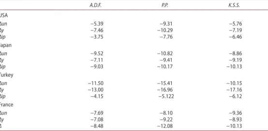
In the second step of the econometric analysis, three unit root tests were applied for each of the countries (the Augmented Dickey-Fuller (A.D.F.), Phillips Perron (P.P.) and Kapetanios, Shin and Shell (K.S.S.) unit root tests). Unit root tests are used to examine whether variables are I(0) or I(1) or not.
Unit root tests are used to analyse whether the series are stationary I(0) or not. Firstly, the long run relationship between variables is specified by the A.D.F. unit root test and following by the P.P. unit root test. The test results of unit root tests are shown in Table 2 (Δ denotes the first differences of the variables) and the stationary relationship between variables is stressed for all of the countries.
3.1. Non-linear A.R.D.L. results
Tables 3 and 4 indicate the results of short and long-run nonlinear A.R.D.L. results for Japan, France, Turkey and the U.S.A., respectively. There is not enough evidence to reject (6) Δyt = c + 𝛿yt−1+ 𝜗+xt−1+ + 𝜗−xt−1− + m−1 ∑ i=1 𝛽iΔyt−1+ n−1 ∑ i=0 (𝜋+ � j Δx + t−1+ 𝜋 −� i Δx + t−1) + et
Table 1. Descriptive statistics.
source: authors’ estimations.
y(France) inf(France) un(France) y(Japan) inf(Japan) un(Japan) mean 1.063442 1.422628 1.036025 1.088486 2.028147 1.016619 std. Dev. 0.318667 0.955391 0.401884 0.424035 0.654926 0.701493 skewness 0.506352 0.767356 1.184816 0.526956 1.030962 0.978665 kurtosis 0.852886 1.075119 1.256409 1.025908 0.950118 1.163947 jarque-Bera 1.007154 1.11368 1.208710 1.2047506 1.73031 2.010047 observations 46 46 46 56 56 56
y(turkey) inf(turkey) un(turkey) y(U.s.a.) inf(U.s.a.) un(U.s.a.) mean 1.070542 1.484159 1.011869 1.054481 1.109345 1.009966 std. Dev. 0.569261 0.592453 0.521891 0.428791 0.756564 0.670397 skewness −0.496924 0.320969 −0.681015 0.093774 0.284906 1.559907 kurtosis 0.724228 0.77040 0.601596 0.814678 0.63212 0.985798 jarque-Bera 1.528560 1.11115 1.59544 1.161654 1.78289 1.67383 observations 56 56 56 56 56 56
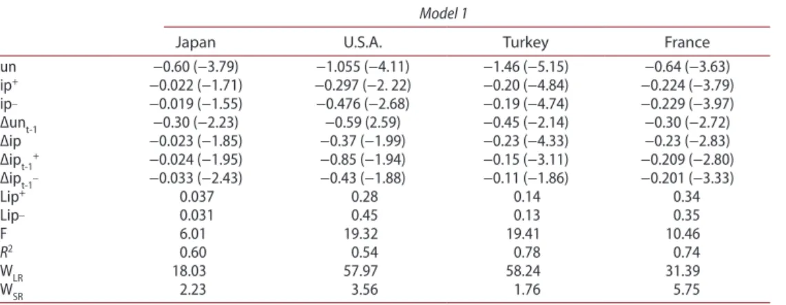
the long-run relationship between inflation and unemployment. According to the results, the Wald test statistics are above the critical value (Wlr defines the Wald test of long run symmetry while Wsr signifies the Wald test of the additive short-run symmetry condition. Lip+ and Lip_ denote positive and negative changes in inflation in the long-run, respectively. un figures the rate of unemployment. ip+ and ip− denote positive and negative changes in
inflation, respectively). This shows that there is a long run relationship between inflation and unemployment in France, Japan, Turkey and the U.S.A.
It must be specified that asymmetric relationships are crucial to emphasise rigidities in the labour markets of the countries. A symmetric relationship implicitly rests on the notion that inflation increment and decrement have the same impact on unemployment. Tables 3 and 4 show our estimation results. As seen in the Tables 3 and 4, ‘downward’ or ‘upward’ unemployment rigidities can be stated for France, Japan, Turkey and the U.S.A.
According to the first model, in a state of instant economic shock, the estimated long term positive effect of inflation for Japan is 0.037 while the estimated negative effect is 0.031. The findings for the U.S.A. are 0.28 and 0.45, for Turkey these estimations are 0.14 and 0.13, for France the results are 0.34 and 0.35, respectively. This points out that for Japan the increase in inflation by 27.02% reduces unemployment by 1% while the decrease in inflation by 32.25 increases unemployment by 1%. These associated figures for the U.S.A. are 3.57, 2.22; for Turkey 7.14, 7.69 and for France 2.94%, 2.85%, respectively. In other meanings, the adjust-ment coefficients of France, Japan, Turkey and the U.S.A. labour markets are respectively, 2.94, 27.02, 7.14, 3.57 which means labour markets in France, Japan, Turkey and the U.S.A. turn their long run equilibrium after 2.94, 27.02, 7.14 and 3.57 period, respectively (Table 3).
Thus, there is enough evidence to conclude that there is the long run negative relationship between inflation and unemployment for France, Japan, Turkey and the U.S.A. Contrarily to this finding, Tang and Bethencourt (2017) aimed to examine the nonlinear structure of the output-unemployment relationship in the 17 Eurozone countries and they found long run and short run symmetric trade-off between output and inflation for France in their study.
The second econometric model (Table 4) presents sufficient evidence for nonlinear link-age between unemployment and economic growth by using the nonlinear A.R.D.L. method.
Table 2. a.D.F., P.P., k.s.s. test results.
source: authors’ estimations.
A.D.F. P.P. K.S.S. Usa ∆un −5.39 −9.31 −5.76 ∆y −7.46 −10.29 −7.19 ∆ip −3.75 −7.76 −6.46 japan ∆un −9.52 −10.82 −8.86 ∆y −7.11 −9.41 −9.19 ∆ip −9.03 −10.17 −10.13 turkey ∆un −11.50 −15.41 −10.15 ∆y −13.00 −16.96 −17.16 ∆ip −4.15 −5.122 −6.12 France ∆un −7.69 −8.10 −9.36 ∆y −7.08 −9.22 −8.93 ∆ −8.48 −12.08 −10.13
As reported by asymmetric test decisions, there is enough the evidence to reject the null hypothesis of the long run asymmetric relationship between macroeconomic variables like economic growth, unemployment.
In a state of economic shock, the long term positive effect of economic growth for France is 0.29 while the negative effect is 0.21. The results for Japan are 5.64 and 8.46; for Turkey 0.82 and 1.44; for the U.S.A. 1.45 and 1.32, respectively. This signifies that for France, 3.44% economic upturn is necessary to decrease unemployment 1% while 4.67% economic down-turn causes an increase in unemployment of 1%. The results for Japan are 1.17 and 1.11; for Turkey 1.21 and 0.69; for the U.S.A. 0.68 and 0.75, respectively.
As support for our results, according to Saglio and López Villavicencio (2012), nominal wages represent less elasticity in the U.S.A. Heyer, Reynès, and Sterdyniak (2007) also stress that nominal wages illustrate more rigidity in the U.S.A. than the European economy.
The asymmetric relationship reflects the opinion that long and short run adjustment speed is low in the France, Japan, Turkey and the U.S.A. Therefore, labour markets in France, Japan, Turkey and the U.S.A. don’t have the inclination of turning their initial case after an economic shock. At this state, the 2007–2008 economic crisis whose effect on American
Table 3. Econometric results for japan, the U.s.a., turkey and France (model 1).
source: authors’ estimations.
Model 1
Japan U.S.A. Turkey France
un −0.60 (−3.79) −1.055 (−4.11) −1.46 (−5.15) −0.64 (−3.63) ip+ −0.022 (−1.71) −0.297 (−2. 22) −0.20 (−4.84) −0.224 (−3.79) ip_ −0.019 (−1.55) −0.476 (−2.68) −0.19 (−4.74) −0.229 (−3.97) Δunt-1 −0.30 (−2.23) −0.59 (2.59) −0.45 (−2.14) −0.30 (−2.72) Δip −0.023 (−1.85) −0.37 (−1.99) −0.23 (−4.33) −0.23 (−2.83) Δipt-1+ −0.024 (−1.95) −0.85 (−1.94) −0.15 (−3.11) −0.209 (−2.80) Δipt-1_ −0.033 (−2.43) −0.43 (−1.88) −0.11 (−1.86) −0.201 (−3.33) Lip+ 0.037 0.28 0.14 0.34 Lip_ 0.031 0.45 0.13 0.35 F 6.01 19.32 19.41 10.46 R2 0.60 0.54 0.78 0.74 WLR 18.03 57.97 58.24 31.39 WsR 2.23 3.56 1.76 5.75
Table 4. Econometric results for japan, U.s.a., turkey and France (model 2).
source: authors’ estimations.
Model 2
Japan U.S.A. Turkey France
un −0.108 (−4.12) −0.69 (−5.83) −0.58 (−1.77) −1.54 (−4.25) y+ −0.60 (−2.95) −1.01 (−2.07) −0.48 (−3.63) −0.45 (−1.87) y_ −0.91 (−4.85) −0.92 (−2.14) −0.84 (−4.65) −0.33 (−1.56) Δunt-1 −0.32 (−2.58) −0.24 (−1.91) −0.91 (−3.25) −0.80 (−3.38) Δy −1.22 (−3.82) −2.38 (−2.71) −0.20 (−1.85) −0.68 (−2.52) Δyt-1+ −1.88 (−3. 87) −2.90 (−3.11) −1.63 (−3.27) −0.35 (−1.82) Δyt-1_ −0.64 (−1.88) −3.25 (−3.95) −0.16 (−1.98) −0.188 (−0.97) Ly+ 5.64 1.45 0.82 0.29 Ly_ 8.46 1.32 1.44 0.214 F 8.98 12.56 11.96 6.06 R2 0.68 0.71 0.72 0.66 WLR 27.95 37.69 35.18 18.19 WsR 3.81 2.53 1.46 0.933
economy has been mostly discussed should be indicated. The crisis has influenced the American labour market inversely.
The existence of a negative relationship between unemployment and inflation is one of the most discussed subjects of macroeconomic policy. Especially, the asymmetric relationship between inflation and unemployment is the mostly accentuated macroeconomic point. For instance, Nguyen and Shin (2011) stresses that American economic recovery at about 10.3% leads to diminished unemployment nearly at the rate of 1. Similarly, Bildirici and Ozaksoy (2014) emphasise that roughly 15% economic recovery is conducive to reducing unemployment by 1%. This study implies the necessity of diminishing unemployment at the rate of nearly 1% to build economic recovery at the point of approximately 64, 36 and 59% respectively in American, Japanese and Turkish labour markets. This is an expected outcome. This study aims to make a contribution to literature by analysing the asymmetric relationship in American, Japanese and Turkish labour markets.
As Shin, Yu, and Greenwood-Nimmo (2013) highlight, the American labour market represents an exceptional instance, because of its flexible labour market, which has a speedy adjustment mechanism and because of this, the economy eliminates the effects of external economic shock. This study supports these findings.
4. Conclusion
This study aims to illuminate the points that potently deliberated for a long time and add an interpretation of the Phillips Curve and conventional perspective of labour markets. The Phillips Curve with its backward bending structure can refer to a positive relationship between the variables. An inversely related pattern of the relationship between inflation and unemployment has a nonlinear structure and this study aims to put emphasis on a linear relationship between the variables besides nonlinear relationship in labour markets which is analysed by the nonlinear A.R.D.L. method.
In this study, the relationship between unemployment and inflation was estimated by nonlinear A.R.D.L. models in France, Japan, Turkey and the U.S.A. By using the nonlinear A.R.D.L. model, the labour market structures of these countries were examined.
In the first model, the long term positive effect of inflation for Japan is 0.037 while the negative effect is 0.031. The findings for the U.S.A. are 0.28 and 0.45, for Turkey are 0.14 and 0.13 and for France these estimations are 0.34 and 0.35, respectively. It points out costly inflationary policy results in a decrease or increase of unemployment at the rate of 1%.
In the second econometric model, the asymmetric relationship between unemployment and economic growth was determined.
According to our results, there is enough evidence to conclude that there is long run negative relationship between inflation and unemployment; unemployment and economic growth for France, Japan, Turkey and the U.S.A.
Disclosure statement
References
Akerlof, G., Dickens, W. T., & Perry, G. L. (2000). Near-rational wage and price setting and the long-run phillips curve. Brookings Papers on Economic Activity, 1, 1–60.
Bachmeier, L. J., & Griffin, J. M. (2003). New evidence on asymmetric gasoline price responses. Review
of Economics and Statistics, 85, 772–776.
Baghli, M., Christophe, C., & Henri, F. (2007). Is the inflation–output Nexus asymmetric in the Euro area? Economics Letters, 94(1), 1–6.
Bildirici, M. (2013). Economic growth and biomass energy. Biomass and Bioenergy, 50, 19–24. Bildirici, M., & Ozaksoy, F. (2014). MURI curve: Alternative approach. International Istanbul Conference
of Economic and Finance. ICEF, Yildiz Technical University
Bildirici, M., & Ozaksoy, F. (2017). The relation between inflation and unemployment with Aardl
analysis (pp. 357–373). Newcastle upon Tyne: Cambridge Scholars Publishing.
Bildirici, M., & Özaksoy, F. (2016). Non-linear analysis of post Keynesian Phillips Curve in Canada labor market. Procedia Economics and Finance, 38, 368–377.
Bildirici, M., & Turkmen, C. (2014). The chaotic relationship between oil return, gold, silver and copper returns in Turkey: Non-linear ARDL and augmented non-linear Granger causality. 4th International Conference on Leadership, Technology, Innovation and Business Management, Yildiz Technical University.
Bildirici, M., & Turkmen, C. (2016). New monetarist Phillips Curve. Procedia Economics and Finance,
38, 360–367.
Chaudhurı, K., Greenwood-Nımmo, M., Kım, M., & Shın, Y. (2013). On the asymmetric U-shaped relationship between inflation, inflation uncertainty, and relative price skewness in the UK. Journal
of Money, Credit and Banking, 45(7), 1431–1449.
Donayre, L., & Panovska, I. (2016). Nonlinearities in the U.S. wage Phillips Curve. Journal of
Macroeconomics, 48, 19–43.
Dritsaki, C., & Dritsaki, M. (2012). Inflation, unemployment and the NAIRU in Greece. International
Conference on Applied Economics (ICOAE) (pp. 118–127).
Eliasson, A.-C. (2001). Is the short-run Phillips Curve nonlinear? Empirical evidence for Australia, Sweden and the United States. Sveriges Riksbank Working Paper Series 124.
Fisher, I. (1926, June). A statistical relation between unemployment and price changes. International
Labor Review, reprinted in Journal of Political EconOTiy (March/Arpil 1973), 496–502.
Friedman, M. (1968). The role of monetary policy. American Economic Review, 58(1), 1–17. Galeotti, M., Lanza, A., & Manera, M. (2003). Rockets and feathers revisited: An international
comparison on European gasoline markets. Energy Economics, 25, 175–190.
Greenwood-Nimmo, M. J., Kim, T. H., Shin, Y., & Van-Treeck, T. (2011). Fundamental asymmetries
in US monetary policymaking: Evidence from a nonlinear autoregressive distributed lag quantile
regression model. Retrieved from http://www.greenwoodeconomics.com/(MG)QT2.pdf
Hasanov, M., Araç, A., & Telatar, F. (2010). Nonlinearity and structural stability in the Phillips Curve: Evidence from Turkey. Economic Modelling, 27(5), 1103–1115.
Heyer, E., Reynès, F., & Sterdyniak, H. (2007). Structural and reduced approaches of the equilibrium rate of unemployment, a comparison between France and the United States. Economic Modelling,
24(1), 42–65.
Huh, H. S., Lee, H. H., & Lee, N. (2008). Nonlinear Phillips Curve, NAIRU and monetary policy rules. Empirical Economics, 37, 131–151.
Humphrey, T. M. (1985). The early history of the Phillips Curve. Federal Reserve Banks – Federal Reserve Bank of Richmond. Economic Review, 71(5), 17–24.
Karantininis, K., Katrakylidis, K., & Persson, M. (2011). Price transmission in the Swedish Pork chain: Asymmetric non-linear ARDL. International Congress, European Association of Agricultural Economists.
Katrakilidis, C., & Trachanas, E. (2012). What drives housing price dynamics in Greece: New evidence from asymmetric ARDL cointegration. Economic Modelling, 29(4), 1064–1069.
Lipsey, R. G. (1960). The relation between unemployment and the rate of change in money wages in the United Kingdom, 1862–1957: A further analysis. Economica, 27(105), 1–31.
Lucas, R. E., Jr. (1972). Expectations and the neutrality of money. Journal of Economic Theory, 4, 103–24.
Lucas, R. E., Jr. (1973). Some international evidence on output – inflation trade-offs. American
Economic Review, 63, 326–34.
Malesevic, L. (2007). Investigating non-linearities in the inflation-growth trade-off in transition countries. Retrieved from http://www.hnb.hr/dub-konf/13-konferencija/malesevic.pdf
Mitchell, W., & Muysken, J. (2008). Chapter 2: Early views on unemployment and the Phillips Curve. Full
employment abandoned: Shifting sands and policy failures. Cheltenham: Edward Elgar Publishing.
Nguyen, V. H., & Shin, Y. (2011). Asymmetric price impacts of order flow on exchange rate dynamics. Melbourne Institute Working Paper Series wp2011n14.
Ozaksoy, F. (2015). Yeni Keynesyen Phillips Eğrisinden MURI’ye emek piyasasında yeni bir bakış. Yayımlanmamış Yüksek Lisans Tezi. Yıldız Teknik Üniversitesi Sosyal Bilimler Enstitütüsü, Supervisor: Prof. Dr. Melike Bildirici.
Palley, T. I. (1997). Does inflation grease the wheels of adjustment? New evidence from the U.S.
Economy. International Review of Applied Economics, 11, 387–398.
Palley, T. (2003). The backward-bending Phillips Curve and the minimum unemployment rate of inflation: Wage adjustment with opportunistic firms. The Manchester School, 71(1), 1463–6786. Palley, T. (2006a). The economics of inflation targeting: Negatively sloped, vertical and
backward-bending Phillips Curve. Economics for Democratic & Open Societies, 1–30.
Palley, T. (2006b). A post-Keynesian framework for monetary policy: Why interest rate operating
procedures are not enough. A handbook of alternative monetary economics. Cheltenham: Edward
Elgar Publishing.
Palley, T. (2008). A backward bending Phillips Curves: A simple model. University of Massachusetts Amherst Working Paper Series, No: 168.
Palley, T. (2009). The economics of the Phillips Curve: Formation of inflation expectations versus incorporation of inflation expectations. Structural Change and Economic Dynamics, 23, 221–230. Pattanaik, S., & Nadhanael, G. V. (2011). Why persistent high inflation impedes growth? An empirical
assessment of theshold level of inflation for India. Reserve Bank of India Working Paper Series, 17. Pesaran, M. H., & Shin, Y. (1999). An autoregressive distributed lag modeling approach to cointegration analysis. In S. Strom (Ed.), Econometrics and economic theory in the 20th century: The Ragnar Frisch
Centennial, 1999 symposium (Chapter 11, pp. 371–413). Cambridge: Cambridge University Press.
https://doi.org/10.1017/CCOL521633230.011
Pesaran, M. H., Shin, Y., & Smith, R. J. (2001). Bounds testing approaches to the analysis of level relationships. Journal of Applied Econometrics, 16, 289–326.
Phelps, E. S. (1967). Phillips Curves, expectations of inflation and optimal unemployment over time.
Economica, 34(135), 254–81.
Phillips, A. W. (1958). The relation between unemployment and the rate of change of money wage rates in the United Kingdom, 1861–1957. Economica, 25(100), 283–299.
Saglio, S., & López-Villavicencio, A. (2012). Introducing price-setting behaviour in the Phillips Curve: The role of non-linearities. MPRA,46646. Retrieved from http://mpra.ub.uni-muenchen.de/46646/ Samuelson, P. A., & Solow, R. M. (1960). Analytical aspects of anti-inflation policy. American Economic
Review Papers and Proceedings, 50(2), 177–194.
Shin, Y., Yu, B., & Greenwood-Nimmo, M. J. (2009). Modelling asymmetric cointegration and dynamic
multipliers in an ARDL framework. Mimeo: University of Leeds.
Shin, Y., Yu, B., & Greenwood-Nimmo, M. J. (2013) Modelling asymmetric cointegration and dynamic multipliers in a nonlinear ARDL framework. In W. C. Horrace & R. C. Sickles (Eds.), Festschrift
in honor of Peter Schmidt. Forthcoming. Retrieved from SSRN https://ssrn.com/abstract=1807745
or https://doi.org/10.2139/ssrn.1807745
Shin, Y., Yu, B., & Greenwood-Nimmo, M. (2014). Modelling asymmetric cointegration and dynamic multipliers in a nonlinear ARDL framework. In W. Horrace & R. Sickles (Eds.), The Festschrift
in Honor of Peter Schmidt.: Econometric Methods and Applications (pp. 281–314). New York, NY:
Springer.
Tang, B., & Bethencourt, C. (2017). Asymmetric unemployment-output tradeoff in the Eurozone.
Tobin, J. (1972). Inflation and unemployment. American Economic Review, 62, 1–26, reprinted in Essays in Economics: Vol. 2, New York, NY: North-Holland, 1975, pp. 33–60.
Van Treeck, T. (2008). Asymmetric income and wealth effects in a non-linear error correction model of
US consumer spending. IMK WP (6). Dusseldorf: Hans- Bockler Foundation.
Wang, P. (2004). The Phillips Curve: Classical, new consensus and post-Keynesian views. Mémoire de maîtrise, Département de Science Economique, Université d’Ottaw, 1–44.
Xu, Q., Niu, X., Jiang, C., & Huang, X. (2015). The Phillips Curve in the US: A nonlinear quantile regression approach. Economic Modelling, 49, 186–197.
Zhang, L. (2017). Modeling the phillips curve in china: A nonlinear perspective. Macroeconomic