Random codes and matrices

(1)

RANDOM CODES AND MATRICES

a dissertation submitted to

the department of mathematics

and the institute of engineering and science

of bilkent university

in partial fulfillment of the requirements

for the degree of

doctor of philosophy

By

˙Ibrahim ¨Ozen

(2)

I certify that I have read this thesis and that in my opinion it is fully adequate, in scope and in quality, as a dissertation for the degree of doctor of philosophy.

Prof. Dr. Alexander A. Klyachko(Supervisor)

Prof. Dr. Sinan Sert¨oz

Prof. Dr. Erdal Arıkan ii

(3)

Prof. Dr. Ferruh ¨Ozbudak

Ass. Prof. Dr. Alex Degtyarev

Approved for the Institute of Engineering and Science:

Prof. Dr. Mehmet B. Baray Director of the Institute

(4)

Merhaba, ho¸s geldin ey ruh-ı revanım merhaba

(5)

ABSTRACT

RANDOM CODES AND MATRICES

˙Ibrahim ¨Ozen Ph.D. in Mathematics

Supervisor: Prof. Dr. Alexander A. Klyachko May, 2009

Results of our study are two fold. From the code theoretical point of view our study yields the expectations and the covariances of the coefficients of the weight enumerator of a random code. Particularly interesting is that, the coefficients of the weight enumerator of a code with random parity check matrix are uncorre-lated. We give conjectures for the triple correlations of the coefficients of weight enumerator of random codes. From the random matrix theory point of view we obtain results in the rank distribution of column submatrices. We give the ex-pectations and the covariances between the ranks (q−rank_{) of such submatrices}

over Fq. We conjecture the counterparts of these results for arbitrary

subma-trices. The case of higher correlations gets drastically complicated even in the case of three submatrices. We give a formula for the correlation of ranks of three submatrices and a conjecture for its closed form.

Keywords: random codes, random matrices, rank, weight enumerator of a random code.

(6)

¨

OZET

RASTSAL KODLAR VE MATR˙ISLER

˙Ibrahim ¨Ozen Matematik, Doktora

Tez Y¨oneticisi: Prof. Dr. Alexander A. Klyachko Mayıs, 2009

Ç alı¸smamızın sonu¸cları iki yönlüdür. Kodlama teorisi a¸cısından, rastsal kodun a˘gırlık polinomunun katsayılarının matematiksel beklentileri ve kovaryansları elde edilmi¸stir. Elde edilen önemli bir sonu¸c, rastsal parite kontrol ile olu¸sturulan kod polinomunun katsayılarının korelasyonunun sıfır olu¸sudur. Rastsal kod polinomu-nun katsayıları arasında ü¸clü korelasyonlar i¸cin varsayım öne sürülmü¸stür. Rast-sal matrisler a¸cısından bakıldı˘gında, rastRast-sal matrisin altmatrislerinin rank beklen-tisi ve aralarındaki kovaryanslar elde edilmi¸stir. Bu sonu¸cların sütun matrislerine sınırlandırılmamı¸s sonu¸cları i¸cin varsayım ileri sürülmü¸stür. Daha yüksek dere-celere bakıldı˘gında, korelasyonların ü¸cüncü derecede ¸cok daha karma¸sıkla¸stı˘gı gözlenmi¸stir. Ü¸cüncü derece korelasyon i¸cin bir toplam formülü elde edilmi¸s, kapalı formu i¸cin sav ileri sürülmü¸stür.

Anahtar s¨ozc¨ukler : rastsal kodlar, rastsal matrisler, rank, rastsal kodun aˇgırlık daˇgılımı.

(7)

Acknowledgement

I would like to express my deepest gratitude to my supervisor Professor Alexander A. Klyachko. His guidance through the work, insightful suggestions and his patience mostly made this study come along.

The department of mathematics in Bilkent university enabled me to keep my chance in spite of many delays. I am grateful to Prof. Mefharet Kocatepe and Prof. Metin G¨urses for the flexibility they showed. I am also obliged to thank to those in the Institute of Science and Engineering that have share in this.

I have received support and encouragement from many friends. I want to thank especially to Murat Altunbulak and Ersin ¨Ureyen for their hospitality during my stays at Ankara. I am also grateful to S¨uleyman Tek and Hatice S¸ahino˘glu for sending me a text which was very critical at the moment.

Finally I thank to my family for their support and encouragement.

(8)

Chapter 1 Introduction

1.1 A Brief Overview of Random Matrices

Study of random matrices has been an efficient way of understanding the average behavior of both mathematical and physical objects.

1.1.1 Complex Random Matrices

Over zero characteristic, the theory of random matrices is mainly developed on eigenvalue statistics. Three basic random matrix ensembles are the Gaussian Orthogonal, Unitary and Symplectic ensembles.

They consist of the sets of n × n

• real symmetric matrices invariant under transformations H → WT

1 HW1,

• Hermitian matrices invariant under transformations H → W∗

2HW2,

• self dual quaternion real matrices invariant under H → WR

3 HW3

respectively, where W1 is an orthogonal, W2 is a unitary and W3 is a symplectic

(11)

CHAPTER 1. INTRODUCTION 2

matrix. W∗ _{(resp. W}R_{) is complex (resp. quaternion) conjugation followed by}

transposition. Recall that a real quaternion q is of the form q = r0+ r1e1+ r2e2+

r3e3, with conjugate ¯q = r0 − r1e1 − r2e2 − r3e3, where ri’s are real. They form

an algebra over real numbers by the multiplication rules e2

1 = e22 = e23 = −1,

e1e2 = e3, e2e3 = e1, e3e1 = e2. A matrix Q = [qij] with real quaternion elements

has the dual matrix QR _{= [¯}_q

ji] and Q is self dual when we have Q = QR.

Symplectic group is the set of real quaternion matrices W such that W−1 _{= W}R_.

In these ensembles, probabilities to have eigenvalues within unit intervals cen-tered at (λ1, λ2, . . . , λn) are known. Correlations of eigenvalues of such matrices

are extensively studied ([20, 6]).

While the initial aim was to understand the energy levels of complex nuclear systems, later developments indicated that eigenvalues of random matrices have similar statistics as the nontrivial zeros of Riemann zeta function ([22, 25]). So, the study of correlations of characteristic polynomials became important to un-derstand the value distribution of this function([15, 5]).

Assuming Riemann Hypothesis Montgomery showed that the two point cor-relation function of Riemann zeta function in the zero mean scaling is similar to two point correlation function for eigenvalues of Circular unitary ensemble in the limit of large matrix size.

Assuming Riemann hypothesis let 1/2+iγj be the nontrivial zeros in the upper

half plane and write ˜γj = γjlog(γj/2π). Montgomery conjectured that distances

˜

γj− ˜γi have the same distribution as arguments of eigenvalues of a large unitary

matrix. He proved a weak version of this in ([22]).

Katz and Sarnak ([14]) proved Montgomery’s conjecture for L functions of algebraic curves over finite fields. The three classical ensembles above appear as the monodromy groups of families of algebraic curves.

Monodromy groups also control the number of rational points. Curves with many rational points are essential for constructing algebaraic geometric codes. It turns out that the families of curves with irreducible monodromy group have big

(12)

number of rational points ([13]).

1.1.2 Random matrices over finite fields

Over positive characteristic, random matrix theory switches from the eigenvalue statistics to the conjugacy class properties of square matrices Mat(n, q) over Fq,

GL(n, q) and the classical groups O(n, q), U(n, q) and Sp(2m, q). The problems studied include the proportion of matrices that have equal minimal and character-istic polynomials (cyclic matrices), that have charactercharacter-istic polynomial free from multiple roots (separable matrices), the same property for minimal polynomial (semisimple matrices).(See ([7]) for example.)

Stong ([26]) showed that the expectation and the variance of the number of different irreducible factors in the characteristic polynomial of a random matrix in GL(n, q) are asymptotically

log(n) + O(1).

Goh and Schmutz ([11]) proved that the distribution is asymptotically normal. Borodin ([2]) studied the distribution of sizes s1 ≥ s2 ≥ . . . of the Jordan

blocks of upper triangular matrices over Fq . He showed that asymptotically as

n → ∞ any finite initial segment of the random vector (s1, s2, . . .) is normally

distributed with mean (p1, p2, . . .) and covariance matrix with entries cij = δijpi−

pipj where pi = 1/qi−1− 1/qi.

1.2 Random codes

Random codes are closely related with the random matrices over finite fields. Specifically, parameters of random codes depend on the distribution and the correlations between the ranks of submatrices.

A linear code C is a linear subspace of Fn

q where Fqis a finite field of q elements.

(13)

of information symbols of the code. The number of nonzero coordinates of a code vector e is said to be the weight |e| of e. Minimum of the weights of nonzero code vectors in C is the minimum distance of the code and it is usually denoted by d. We call a code with parameters n, k, d over Fq an [n, k, d]q code.

If we consider Fn

q as a linear space with the standard scalar product hu, vi =

P

iuivi, then the orthogonal complement C⊥ of C is called the dual code to C.

Let C be an [n, k]q code and fix a basis {bi} of C. Let G be a k × n matrix

whose rows consist of the basis vectors bi of C. Then any element e ∈ C is a

linear combination of row-vectors of G. We call G a generator matrix of C. G is also an important matrix for the dual code C⊥_{. Since any vector e}0 _{∈ C}⊥ _is

orthogonal to the basis vectors of C, the product G × (e0₎T _{is the zero vector and}

this is the criterion for lying in C⊥_{. G is called a parity check matrix of the code}

C⊥_.

Let C ⊂ Fn

q be a code and let Ai be the number of code vectors with exactly

i nonzero coordinates

Ai = |{e ∈ C : |e| = i}|.

Then we define the weight enumerator WC(t) of the code C as the polynomial

WC(t) =

X

i

Aitn−i. (1.1)

We find the following form of the weight enumerator vital for our purposes (see [27])

WC(1 + t) =

X

I⊂{1,2,...,n}

qk−rIt|I|, (1.2)

where rI is rank of the column submatrix of G, spanned by the columns indexed

by I.

All the parameters of codes can be extracted from the weight enumerator WC(t) which is given by the rank function q−rI, I ⊂ {1, 2, . . . , n}, of the generator

matrix. A code can be considered as a configuration of points (columns of the generator matrix) in the projective space. Then existence of a code with given weights turns out to be equivalent to existence of a configuration with given

(14)

rank function as we see in Equations (1.1) and (1.2). But this is a classical wild problem and it can be arbitrarily complicated ([21]). So we pass to the statistical approach rather than trying to determine the explicit structure.

Existence of a code with parameters n, k, d over Fq amounts to simultaneous

vanishing of the coefficients

A1 = A2 = . . . = Ad−1 = 0.

This involves the joint distribution of the coefficients of the weight enumerator. Given the relation between the rank functions and the code weights, it is a natural course of action to study the statistics of the rank functions. The main results of this work are the explicit formulas for the expectation and the covariances between the rank functions of random matrices. They provide the answers to the counterpart problems for the code weights. In particular we find out that the coefficients of weight enumerator of a code constructed by random parity check matrix are uncorrelated.

For a matrix G, we take randomness in the sense that the entries are inde-pendent and they are uniformly distributed along the field Fq. One can easily

deduce from Equation (3.5) that probability of a square n × n matrix over Fq

to be singular is positive even when n → ∞, while for a k × n matrix with R = k/n < 1 the matrix is almost sure to have maximal rank k. Hence we will tacitly assume maximality of the rank when fixing a random k × n matrix with k/n < 1. One must keep in mind that there are two ways that a random matrix gives rise to a code. Once we are given a k × n matrix G there is the [n, k]q

code which assumes G as its generator matrix; and the second, the code which assumes G as its parity check matrix. Both codes will be referred as random code. We denote the random code in the first sense by C and the code in the second sense by C⊥_{. Their weight enumerators will be referred as W}

C(t) = P iAitn−i and W_C⊥(t) = P iA⊥i tn−i respectively.

Throughout the text G is a random k × n matrix over the finite field Fq.

We denote its rank, considered as a random quantity, by rk×n. When we deal

with column sub-matrices we refer to the matrix as GI and its rank by rI, where

(15)

1.3 Statement of Results

Results in this thesis have been published online with the DOI reference 10.1016/j.ffa.2009.03.002 ([18]).

Our main results are as follows. The sth moment of the rank function q−rk×n

of a k × n random matrix is given by µs(q−rk×n) = q−kn X 0≤r≤k qr(n−s) · k r ¸ Y 0≤i<r (1 − q−n+i_), µs(q−rk×n) = Y 0≤i<k (q−n+ q−s− q−n−s+i),

where the product in the second formula is noncommutative in x = q−n _{and y =}

q−s _{with the commutation rule yx = qxy. The moment µ}

s(q−rk×n) is symmetric

in n and k. Furthermore if s is a nonnegative integer then it is also symmetric in s. For example the expectation of q−rk×n _{is given by}

E(q−rk×n) = q−n+ q−k− q−n−k.

The covariance between the rank functions q−rI _{and q}−rJ _{of two column}

sub-matrices is given by

cov(q−rI, q−rJ) = (q − 1)(q

k_{− 1)(q}|I∩J|_{− 1)}

q2k+|I|+|J| .

One may ask about the covariance between the rank functions q−rKI _{where r} KI

denotes rank of the submatrix spanned by the row set K and the column set I. We conjecture that

cov(q−rLI_{, q}−rM J_{) =} (q − 1)(q|I∩J|− 1)(q|L∩M |− 1)

q|I|+|J|+|L|+|M | . (1.3)

Next we show that the covariances between the coefficients of weight enumer-ator of the random code C⊥ _{are given by}

cov(W_C⊥(x), W_C⊥(y)) = X i,j cov(A⊥ i , A⊥j )xn−iyn−j = (q − 1)(q n−k_{− 1)} q2(n−k) ((xy + q − 1) n_{− (xy)}n_).

(16)

An important corollary of this theorem is that the coefficients of weight enumera-tor of the code C⊥_{with random parity check matrix are uncorrelated. This result}

is not valid for the code C given by random generator matrix.

We also studied the triple correlations between the ranks of three submatri-ces. Using the classification of triplets of subspaces we managed to deduce an extremely complicated formula. To our surprise computer experiments show be-yond reasonable doubt that the formula is equivalent to a simple closed one. It is even simpler when we switch from the correlations to the cumulants. We conjec-ture that the closed formula of the joint cumulant of ranks of three submatrices is given by σ(q−rI_{, q}−rJ_{, q}−rK_{) =} (q − 1)2(qk− 1) q3k+I+J+K ¡ qIJ+JK+KI−IJK _{− (q}IJ _{+ q}JK _{+ q}KI₎ + 2 + (qk_{− q)(q}IJK _{− 1)}¢_,

where on the right hand side of the equation the multiplicative notation for sets like IJ means the cardinality of their intersection |I ∩ J|. We remind that the joint cumulant of a triplet of random variables is

σ(X, Y, Z) = E(XY Z) − E(X)cov(Y, Z) − E(Y )cov(Z, X) −E(Z)cov(X, Y ) − E(X)E(Y )E(Z).

This conjecture is equivalent to the following formula for joint cumulants of the coefficients of W_C⊥(t), σ(W_C⊥(x), W_C⊥(y), W_C⊥(z)) = X i,j,l σ(A⊥ i , A⊥j , A⊥l )xn−iyn−jzn−l = q−3(n−k)_{(q − 1)}2_(qn−k_{− 1)} ( ¡ xyz + (q − 1)(x + y + z + q − 2)¢n− (xyz)n

−((xy + q − 1)n_{− (xy)}n_)zn_{− ((yz + q − 1)}n_{− (yz)}n_)xn

−((zx + q − 1)n− (zx)n)yn+ (qn−k− q) h

(xyz + q − 1)n− (xyz)n i)

(17)

For the random code C the corresponding equation is σ(WC(x), WC(y), WC(z)) = (q − 1)2(qk− 1) n q−n_{(xyz + q − 1)}n − q−2n¡(xy + q − 1)n(z + q − 1)n+ (yz + q − 1)n(x + q − 1)n + (zx + q − 1)n_{(y + q − 1)}n¢_{+ 2q}−3n_{(x + q − 1)}n_{(y + q − 1)}n_{(z + q − 1)}n + (qk_{− q)}£_q−2n_{(xyz + (q − 1)(x + y + z + q − 2))}n − q−3n(x + q − 1)n(y + q − 1)n(z + q − 1)n¤o.

There exists a classification of quadruples of subspaces due to Gelfand and Ponomarev ([10]). For further study of this subject, one may wonder whether it may lead to a closed formula for the quadruple correlations.

The above results on correlations imply, for example, that the roots of weight enumerator WC(1 + z) of a selfdual code C = C⊥ are almost sure to be on the

circle z = |√q|, provided q > 9. Here by almost sure we mean that the probability to have a root off the circle tends to 0 as n → ∞. Similar but less sharp results hold for all [n, k]q codes where q > q0(R), R = k/n ([17]).

The thesis is organized as follows. Chapter 2 is a survey to summarize the well known results over finite fields. Results mentioned in this chapter are not used nor needed to proceed to the rest of the thesis.

In Chapter 3 we evaluate the moments and the covariances between the rank functions. Moments are given by Theorem (3.3). We derive the covariance be-tween the ranks of two submatrices in Theorem (3.6). Using this, we show that the coefficients of the weight enumerator of the random code C⊥_{are uncorrelated}

by Theorem (3.10) and Corollary (3.11).

In Chapter 4 we study the triple correlations between the coefficients of the weight enumerators. To proceed in this direction we need the triple correlations between the ranks of three submatrices. A triplet of submatrices gives a triplet of subspaces. We review the classification of triplets of subspaces and obtain the number of triplets with given invariants. This enables us to obtain a formula for the triple correlations between the ranks of three submatrices which is given by Theorem (4.7). The main Conjecture (4.8) provides the closed form of the joint

(18)

cumulant of three ranks. Equivalent to this conjecture we give Corollaries (4.10) and (4.11) on the joint cumulant of coefficients of WC(t) and WC⊥(t) respectively.

(19)

Chapter 2 Known Results Over Finite

Fields

Random matrix theory over finite fields focuses on conjugacy classes of random elements of the classical groups. Some of the properties that are invariant for the same class are separability, semisimplicity, being cyclic, number of Jordan blocks and so on. Similarity classes of matrices in Mat(n, q) and GL(n, q) are well known, conjugacy classes in O(n, q), U(n, q) and Sp(2n, q) are studied by Wall ([30]).

We remind the reader that our purpose is to provide a survey. Results of this chapter won’t be used in the rest of the thesis.

2.1 Results for Mat(n, q) and GL(n, q)

2.1.1 Similarity Classes

Similarity classes of matrices in Mat(n, q) are given by the rational canonical form. For a monic polynomial φ(z) = zm_{+ a}

m−1zm−1+ . . . + a1z + a0 define the

(20)

CHAPTER 2. KNOWN RESULTS OVER FINITE FIELDS 11 companion matrix C(φ) to be C(φ) =          0 1 0 . . . 0 0 0 1 . . . 0 ... 0 0 0 . . . 1

−a0 −a1 −a3 . . . −am−1

         . (2.1)

A matrix A ∈ Mat(n, q) is said to be in rational canonical form if it is the direct sum of companion matrices of nonscalar monic polynomials φi

A =        C(φ1) 0 0 . . . 0 0 C(φ2) 0 . . . 0 ... 0 0 0 . . . C(φt)        (2.2)

such that φi+1| φi. Any matrix is similar to a unique matrix in rational form.

This form follows from the fact that the space on which A acts decomposes as direct sum of cyclic subspaces. So A is cyclic if and only if its rational form is companion matrix C(φ) of a polynomial φ.

One can parameterize a similarity class by a collection of monic irreducible polynomials {pi} with corresponding partitions of natural numbers λi = λi,1 ≥

λi,2 ≥ . . . satisfying _X

i

|λi| deg(pi) = n. (2.3)

Rational form of such a class is given by the matrix        C(Q_ipλi,1_i ) 0 0 . . . 0 0 C(Q_ipλi,2_i ) 0 . . . 0 ... 0 0 0 . . . C(Q_ipλi,t_i )        . (2.4)

Characteristic polynomial of any matrix in the class is given by Q_ip|λi|_i .

For the conjugacy classes of GL(n, q) the only restriction is that characteristic polynomial can not have z as a factor, so |λz| = 0.

(21)

CHAPTER 2. KNOWN RESULTS OVER FINITE FIELDS 12

Let A ∈ Mat(n, q) with characteristic polynomial φ(z). If φ completely factors in Fq then similarity the class of A is given by the Jordan form. To describe it

define Jc to be the elementary Jordan matrix with characteristic value c

Jc =          c 0 . . . 0 0 1 c . . . 0 0 ... ... ... ... ... 0 0 c 0 0 0 . . . 1 c          . (2.5)

Now let p be an irreducible polynomial over Fq with roots in the closure of the

field β, βq_{, β}q2

, . . . , βdeg p−1_{. For any natural number λ we define the companion}

matrix Jp,λ as Jp,λ =        Jβ 0 . . . 0 0 Jβq . . . 0 0 ... ... ... ... ... 0 0 . . . 0 J_βdeg p−1        , (2.6)

where each J is a λ×λ Jordan matrix with the corresponding characteristic value. Suppose the similarity class of A has data pi and λi. Then A is similar to a

matrix A =          Jp1,λ1,1 0 . . . 0 0 0 Jp1,λ1,2 . . . 0 0 ... ... ... ... ... 0 0 Jpi,λi,1 . . . . ..          . (2.7)

2.1.2 Cycle Indices

Cycle indices for Mat(n, q) and GL(n, q) are first introduced by Kung and Stong. These are polynomials that the cycle structures are encoded in their coefficients. Let xp,λp be variables corresponding to pairs of monic irreducible polynomials p

(22)

and corresponding partitions of natural numbers |λp|. Then one defines the cycle

index generating function of GL(n, q) as the power series 1 +X n un |GL(n, q)| X α∈GL(n,q) Y p6=z xp,λp(α)

where the product is over all monic irreducible polynomials over Fq. Cycle index

for Mat differs only in including the polynomial z in the product.

Stong gives a factorization for the cycle index, using a quantity cGL,p,q(λ). For

a partition λ with mi parts of size i, define

di = m11 + m22 + . . . + mi−1(i − 1) + (mi+ mi+1+ . . .)i.

For empty partition λ set cGL,p,q(λ) = 0, otherwise

cGL,p,q(λ) = Y i mi Y l=1

(qdeg(p)di_{− q}deg(p)(di−l)_). _(2.8)

Then the cycle index generating functions of GL(n, q) and Mat(n, q) have the following factorizations respectively

We need a few lemmas that will be useful in deriving results from the cycle indices. In the following we use the notation [un_{]f (u) to denote the coefficient of}

un _{in the Taylor expansion of f (u) around 0.}

Lemma 2.1 If f (1) < ∞ and the Taylor series of f around 0 converges at u = 1, then

lim

n→∞[u

n_]f (u)

1 − u = f (1). (2.11)

Proof. Let f (u) =P∞_n=0anun. Then

f (u) 1 − u = Ã ∞ X i=0 ui ! Ã ∞ X n=0 anun ! = ∞ X n=0 ( n X i=0 an−i)un.

(23)

CHAPTER 2. KNOWN RESULTS OVER FINITE FIELDS 14 Lemma 2.2 Y p µ 1 − udeg(p) qdeg(p)t ¶ = 1 − u qt−1, (2.12)

where the product is over all monic irreducible polynomials over Fq.

Proof. Assume that t = 1 and let v = u

q. Then using 1 1 − vdeg(p) = ∞ X i=0 (vdeg(p))i we get Y p 1 1 − vdeg(p) = X ip vdeg(Qppip).

So coefficient of vd_{is the number of monic polynomials of degree d, which is equal}

to qd_{. Hence when we pass to u notation we get}

1 1 − udeg(p) qdeg(p) = ∞ X d=0 ud₌ 1 1 − u.

So for t = 1 we get the result and the general case follows by changing u to

u qt−1. Lemma 2.3 Y p6=z ∞ Y r=1 µ 1 − udeg(p) qdeg(p)r ¶ = 1 − u, (2.13)

where p runs through monic irreducible polynomials not equal to z. Proof. By the previous lemma we get

Y p6=z ∞ Y r=1 µ 1 − udeg(p) qdeg(p)r ¶ = ∞ Y r=1 Ã 1 − u qr−1 1 − u qr !

and the cancelations bring the result.

Gordon’s generalization of Rogers-Ramanujan identities [cite] gives the fol-lowing corollary that will be used later

∞ Y r=1 µ 1 − 1 qr deg(p) ¶ X λ:λ1<k 1 cGL,p,q(λ) = ∞ Y r=1 r=0,±k(mod2k+1) µ 1 − 1 qr deg(p) ¶ . (2.14)

(24)

Now we are ready to show how the cycle index machinery is used. For large matrices probability of being semi-simple, cyclic and separable matrices will be obtained.

Theorem 2.4 As n → ∞, probability that a random element of Mat(n, q) is semi-simple tends to ∞ Y r=1 r=0,±2(mod5) µ 1 − 1 qr−1 ¶ . (2.15)

Proof. Semi-simplicity of a matrix in Mat(n, q) is equivalent that Jordan form has no block of size greater than 1. So that partitions of the similarity class satisfy λ1 < 2. Cycle index for Mat and its factorization is

1 +X n un |GL(n, q)| X α∈GL(n,q) Y p xp,λp(α) = Y p X λ xp,λ u|λ| deg(p) cGL,p,q(λ) ,

where the products are over all monic irreducible polynomials over Fq. If we

set xp,λp = 1 for those pairs with the partition satisfying λ1 < 2 and xp,λp = 0

otherwise, we get X

n

un|(semisimple matrices in Mat(n, q))|

|GL(n, q)| =

on the left hand side. Hence limiting probability becomes limn→∞ |GL(n, q)| qn2 [u n_]Y p X λ:λ1<2 u|λ| deg(p) cGL,p,q(λ) = Eq.2.13 lim n→∞ |GL(n, q)| qn2 [u n_] Q p ³Q_∞ r=1 ³ 1 − udeg(p) qr deg(p) ´ P λ:λ1<2 u|λ| deg(p) cGL,p,q(λ) ´ (1 − u)Q∞_r=1 ³ 1 − u qr ´ = Eq.2.11 Y p Ã_∞ Y r=1 µ 1 − 1 qr deg(p) ¶ X λ:λ1<2 1 cGL,p,q(λ) ! = Eq.2.14 ∞ Y r=1 r=0,±2(mod5) µ 1 − 1 qr−1 ¶ .

(25)

Probability to get semi-simple element in GL(n, q) is given by the next theo-rem.

Theorem 2.5 As n → ∞, probability that a random element of GL(n, q) is semi-simple tends to ∞ Y r=1 r=0,±2(mod5) ³ 1 − 1 qr−1 ´ ³ 1 − 1 qr ´ . (2.16)

Proof. In the cycle index of GL(n, q) we set xp,λp = 1 if λ satisfies λ1 < 2 and

xp,λp = 0 otherwise. This gives the desired probability on the right hand side and

it is equal to lim n→∞[u n_]Y p6=z X λ:λ1<2 u|λ| deg(p) cGL,p,q(λ) = Eq.2.13 lim n→∞[u n_] 1 1 − u Y p6=z Ã ∞ Y r=1 µ 1 − u deg(p) qr deg(p) ¶ X λ:λ1<2 u|λ| deg(p) cGL,p,q(λ) ! = Eq.2.11 Y p6=z Ã_∞ Y r=1 µ 1 − 1 qr deg(p) ¶ X λ:λ1<2 1 cGL,p,q(λ) ! = Eq.2.14 Y p6=z ∞ Y r=1 r=0,±2 (mod5) µ 1 − 1 qr ¶ = ∞ Y r=1 r=0,±2 (mod5) 1 ³ 1 − 1 qr ´Y p ∞ Y r=1 r=0,±2 (mod5) µ 1 − 1 qr ¶ = ∞ Y r=1 r=0,±2 (mod5) ³ 1 − 1 qr−1 ´ ³ 1 − 1 qr ´ .

Next, we give probabilities that the random element is cyclic.

Theorem 2.6 As n → ∞, probability that a random element in Mat(n, q) is

cyclic tends to _µ 1 − 1 q5 ¶_Y∞ r=3 µ 1 − 1 qr ¶ .

(26)

Proof. A matrix is cyclic if and only if all the partitions in its rational canonical form have at most one part. Once again manipulating cycle index accordingly, we obtain the probability as

lim n→∞ |GL(n, q)| qn2 [u n_]Y p Ã 1 + ∞ X j=1 uj deg(p) qj deg(p)−deg(p)_(qdeg(p)_{− 1)} ! = Eq.2.12 ∞ Y r=1 µ 1 − 1 qr ¶ lim n→∞[u n_] Q p ³ 1 − udeg(p) qdeg(p) ´ ³ 1 +P∞_j=1 uj deg(p) qj deg(p)−deg(p)_(qdeg(p)₋₁₎ ´ 1 − u = Eq.2.11 ∞ Y r=1 µ 1 − 1 qr ¶ Y p µ 1 + 1 qdeg(p)_(qdeg(p)_{− 1)} ¶ = Eq.2.12 ∞ Y r=3 µ 1 − 1 qr ¶ Y p µ 1 − 1 q6 deg(p) ¶ = µ 1 − 1 q5 ¶_Y∞ r=3 µ 1 − 1 qr ¶ .

Theorem 2.7 As n → ∞, probability that a random element of GL(n, q) is cyclic tends to 1 − 1 q5 1 + 1 q3 .

Proof. Proof is similar to the previous case.

Now we give the probabilities that a random element is separable.

Theorem 2.8 As n → ∞, probability that a random element of Mat(n, q) is separable tends to ∞ Y r=1 µ 1 − 1 qr ¶

(27)

size 1. So we get the probability from the cycle index as lim n→∞ |GL(n, q)| qn2 [u n_]Y p µ 1 + udeg(p) qdeg(p)_{− 1} ¶ = Eq.2.12 lim n→∞ |GL(n, q)| qn2 [u n_] Q p ³ 1 + udeg(p) qdeg(p)₋₁ ´ ³ 1 − udeg(p) qdeg(p) ´ 1 − u = Eq.2.11 ∞ Y r=1 µ 1 − 1 qr ¶ .

Theorem 2.9 As n → ∞, probability that a random element of GL(n, q) is separable tends to

1 −1 q

Proof. Cycle index of GL(n, q) and the condition on the partitions give the prob-ability lim n→∞[u n_]Y p6=z µ 1 + udeg(p) qdeg(p)_{− 1} ¶ = Eq.2.12 lim n→∞[u n_] ³ 1 − u q ´ Q p6=z ³ 1 + udeg(p) qdeg(p)₋₁ ´ 1 − u = Eq.2.11 1 − 1 q.

2.2 Results for Other Classical Groups

Unitary Groups: Unitary group U(n, q) is defined as the subgroup of GL(n, q2₎

that preserves a nondegenerate skew linear form. A skew linear form on an n dimensional vector space V over Fq2 is a bilinear map h, i : V × V → F_q2 satisfying hx, yi = hy, xiq_{. One such form is given by hx, yi =}P

ixiyiq. Any two

nondegenerate skew linear forms are equivalent ([4, page 7]), so U(n, q) is unique up to isomorphism. Cardinality of the unitary group is given by |U(n, q)| = q(n2) Qn

(28)

Description of conjugacy classes in the classical groups requires combinatorial properties of polynomials. For a polynomial φ(z) ∈ Fq2[z] with nonzero constant term, define ˜ φ(z) = z deg(φ)_φq₍1 z) (φ(0))q ,

where φq_{raises each coefficient of φ to the qth power. A conjugacy class in U(n, q)}

is given by a collection of monic irreducible polynomials p and corresponding partitions λp of nonnegative integers. This collection gives a conjugacy class if

and only if 1. |λz| = 0,

2. λp = λp˜,

3. P_p|λp| deg(p) = n.

Let ˜N(q, d) be the number of monic, irreducible polynomials p(z) ∈ Fq2(z) of degree d such that p = ˜p. The number ˜N(q, d) is given by

˜ N(q, d) = ( 0 if d is even, 1 d P r|dµ(r)(q d r + 1) if d is odd. (2.17) Furthermore, let ˜M(q, d) be the number of unordered pairs of monic, irreducible, degree d polynomials over Fq2, where p 6= ˜p. This number is given by

˜ M(q, d) =        1 2(q2− q − 2) if d = 1, 1 2d P r|dµ(r)(q 2d r − qdr) if d > 1 and d is odd, 1 2d P r|dµ(r)q 2d r if d is even. (2.18)

Symplectic Groups: Symplectic group is defined as as the subgroup of GL that preserves a non-degenerate alternating form. An alternating form on a vector space V over Fq is a bilinear map h, i : V × V → Fq such that hx, yi = −hy, xi.

Alternating forms exist only on vector spaces of even dimension and they are all equivalent, so the Symplectic group Sp(2n, q) is unique up to isomorphism. An example to such forms is hx, yi = P_i(x2i−1y2i− x2iy2i−1). Order of the group

Sp(2n, q) is given by qn2Q_n

(29)

Given a polynomial φ(z) ∈ Fq[z] with non-vanishing constant term, define the

polynomial

(φ)∗_{(z) =} zdeg(φ)φq(1z)

φ(0) .

Conjugacy classes in the Symplectic group Sp(2n, q) are defined by the fol-lowing data on the monic,non-constant irreducible polynomials p ∈ Fq[z] and

corresponding partitions λp of non-negative integers. For p(z) = z ± 1, the

cor-responding partition λ±

p must have an even number of odd parts; and to each

non-zero even part a sign is associated. This data gives a conjugacy class if and only if 1. |λz| = 0, 2. λp = λ(p)∗, 3. P_p=z±1|λ± p| + P p6=z±1|λp| deg(p) = 2n.

Combinatorial properties of polynomials for Sp(2n, q) depends on the parity of characteristic. So define

e(q) = (

2 if q is odd, 1 if q is even.

We also need the number N(q, d) of monic, irreducible polynomials of degree d over Fq. This number is given by

N(q, d) = ( q − 1 if d = 1 1 d P r|dµ(r)q d r if d > 1. (2.19)

Now let N∗_{(q, d) be the number of monic, irreducible, degree d polynomials}

p over Fq such that p = ¯p; and let M∗(q, d) be the number of un-ordered pairs

(30)

numbers are given by

N∗(q, d) =        e(q) if d = 1, 0 if d is odd and d > 1, d−1P r|d, r oddµ(r)(q d 2r + 1 − e(q)) if d is even, (2.20) M∗(q, d) =        1 2(q − e(q) − 1) if d = 1, 1 2N(q, d) if d is odd and d > 1, 1 2 ¡ N(q, d) − N∗_{(q, d)}¢ _{if d is even.} (2.21)

Orthogonal Groups: Orthogonal groups can be defined as subgroups of GL(n, q) that preserves a non-degenerate symmetric bilinear form. We assume that the characteristic is not equal to 2. For n = 2l + 1 odd, there are two such forms up to isomorphism. Their corresponding groups O+_{(2l + 1, q) and}

O−_{(2l + 1, q) are isomorphic, with inner product matrices A and δA, where δ is}

a non-square in Fq and A is given by

A =     1 0 0 0 0l Il 0 Il 0l     .

Order of these groups is given by 2ql2Q_l

i=1(q2i− 1).

For n = 2l even, there are again two forms up to isomorphism with inner product matrices Ã 0l Il Il 0l ! ,       0l−1 Il−1 0 0 Il−1 0l−1 0 0 0 0 1 0 0 0 0 −δ      ,

where δ is a non-square in Fq. If we denote the two orthogonal groups by O+(2l, q)

and O+_{(2l, q), their cardinalities are given by 2q}l2_−l

(ql_{∓ 1)}Ql

(31)

2.2.1 Separable Matrices

Let sG(∞, q) denote limiting probability that a random element in G is separable

as n → ∞ where G is one of the classical groups. Fulman et. al. give the following table of these probabilities ([7]).

Group G q Limiting separability probability sG(∞, q)

GL(n, q) any 1 −1 q U(n, q) any ³ 1 + 1 q ´ Q d odd ³ 1 − 2 qd_(qd₊₁₎ ´_{N (q,d)}˜ any q_q22−1₊₁ Q d odd ³ 1 − 1 (qd₊₁₎2 ´_{N (q,d)}˜ _Q d≥1 ³ 1 + 1 q4d₋₁ ´_{M (q,d)}˜ SP(2m, q) odd ³ 1 −1 q ´₂_Q d≥1 ³ 1 − 2 qd_(qd₊₁₎ ´_N∗_(q,2d) even ³ 1 −1 q ´ Q d≥1 ³ 1 − 2 qd_(qd₊₁₎ ´_N∗_(q,2d) odd q(q−1)_(q2₋₁₎32 Q d≥1 ³ 1 − 1 (qd₊₁₎2 ´_N∗_(q,2d)_Q d≥1 ³ 1 + 1 (q2d₋₁₎ ´_M∗_(q,d) even (q−1)_(q2₋₁₎2 Q d≥1 ³ 1 − 1 (qd₊₁₎2 ´_N∗_(q,2d)_Q d≥1 ³ 1 + 1 (q2d₋₁₎ ´_M∗_(q,d) O(2m + 1, q) any sSp(∞, q) O±_{(2m, q)} _odd _s Sp(∞, q) O±_{(2m, q)} _even 1 2sSp(∞, q)

Table 2.1: Separable matrix limiting probabilities.

They also give the following Table (2.2) of lower and upper bounds for the complicated limiting probabilities sG(∞, q).

Group G q sSp(∞, q) lower bound sSp(∞, q) upper bound

GL(n, q) any 1 − q−1 _{1 − q}−1 U(n, q) any 1 − q−1_{− 2q}−3_{+ 2q}−4 _{1 − q}−1_{− 2q}−3_{+ 6q}−4 2 0.4147 0.4157 3 0.6283 0.6286 Sp(2m, q) odd 1 − 2q−1_{+ 2q}−2_{− 4q}−3_{+ 4q}−4 _{1 − 2q}−1_{+ 2q}−2_{− 4q}−3_{+ 9q}−4 even 1 − 3q−1_{+ 5q}−2_{− 10q}−3_{+ 12q}−4 _{1 − 3q}−1_{+ 5q}−2_{− 10q}−3_{+ 23q}−4 2 0.2833 0.2881 3 0.3487 0.3493

O(2m + 1, q) any same as for sSp(∞, q) same as for sSp(∞, q)

O±_{(2m, q)} _odd _{same as for s}

Sp(∞, q) same as for sSp(∞, q)

even 1

2 bound for sSp(∞, q) 12 bound for sSp(∞, q)

(32)

One can find table of convergence rates for the separability limiting probabil-ities in ([7]).

2.2.2 Cyclic and Regular Matrices

Let cG(∞, q) denote the limiting probability of cyclicness in G as n → ∞. For

the classical groups, the probabilities are given in ([7]) and we take the Table (2.3) of results from there.

Group G q Limiting probability cG(∞, q)

GL(n, q) any (1 − q−5_{)/(1 + q}−3₎ U(n, q) any ³ 1 + 1 q ´ Q d odd ³ 1 − 1 qd_(qd₊₁₎ ´_{N (q,d)}˜ _Q d≥1 ³ 1 + 1 q2d_(q2d₋₁₎ ´_{M (q,d)}˜ any ³ 1 − 1 q2 ´ Q d odd ³ 1 + _q3dq_(qd−1d₊₁₎ ´_{N (q,d)}˜ _Q d≥1 ³ 1 + 1 q6d ´_{M (q,d)}˜ any (q2_q(q−1)(q4₊₁₎3−1) Q d odd ³ 1 + 1 (qd_+1)(q2d₋₁₎ ´_{N (q,d)}˜ _Q d≥1 ³ 1 + 1 (q2d_−1)(q4d₊₁₎ ´_{M (q,d)}˜ Sp(2m, q) any Q_d≥1 ³ 1 − 1 qd_(qd₊₁₎ ´_N∗_(q,2d)_Q d≥1 ³ 1 + 1 qd_(qd₋₁₎ ´_M∗_(q,d) odd _(q2q_+1)(q3(q3−1)4₋₁₎ Q d≥1 ³ 1 + 1 (qd_+1)(q2d₋₁₎ ´_N∗_(q,2d)_Q d≥1 ³ 1 + 1 (qd_−1)(q2d₊₁₎ ´_M∗_(q,d) even _q(qq32−1₊₁₎ Q d≥1 ³ 1 + 1 (qd_+1)(q2d₋₁₎ ´_N∗_(q,2d)_Q d≥1 ³ 1 + 1 (qd_−1)(q2d₊₁₎ ´_M∗_(q,d) O(2m + 1, q) any ³ 1 −1 q ´ cSp(∞, q) O±_{(2m, q)} _odd ³_{1 −}1 q + 2q12 ´ cSp(∞, q) even ³ 1 − 1 2q ´ cSp(∞, q)

Table 2.3: Cyclic matrix limiting probabilities.

Upper and lower bounds for the limiting probabilities are given in Table (2.4). In that table, the constants k1, k2, k3 are given by

k1 = 1 − q−1, k2 = 1 − q−1+ 1 2q −2_, _k 3 = 1 − 1 2q −1_.

One can find tables of convergence rates and limiting probabilities expanded in q−1 _modO(q−10_{) in ([7]).}

An element of a finite classical group G of characteristic p is called regular if its centralizer in the corresponding group over Fqhas minimal possible dimension,

(33)

Group G q cG(∞, q) lower bound cG(∞, q) upper bound

GL(n, q) any (1 − q−5_{)/(1 + q}−3₎ _{(1 − q}−5_{)/(1 + q}−3₎

U(n, q) any (1 − q−3_{)/(1 + q}−4₎ _{1 − q}−3

Sp(2m, q) odd 1 − 3q−3_{+ q}−4_{− q}−5 _{1 − 3q}−3_{+ 2q}−4_{+ q}−5

even 1 − 2q−3_{− q}−5 _{1 − 2q}−3_{+ q}−4_{+ q}−5

O(2m + 1, q) any k1 bound for cSp(∞, q) k1 bound for cSp(∞, q)

O±_{(2m, q)} _odd _k

2 bound for cSp(∞, q) k2 bound for cSp(∞, q)

even k3 bound for cSp(∞, q) k3 bound for cSp(∞, q)

Table 2.4: Explicit bounds for cyclic matrix limiting probabilities.

which is equal to rank of G. For the general linear, unitary and symplectic groups, notions of cyclic and regular elements coincide. For the orthogonal groups, the two concepts are different. Table (2.5) from ([7]) shows the limiting probabilities rG(∞, q) of regular elements in the corresponding orthogonal groups.

Group G q Limiting probability rG(∞, q)

O(2m + 1, q) odd ³ 1 + 1 q2_(q+1) ´ cSp(∞, q) even cSp(∞, q) O±_{(2m, q)} _odd ³_{1 +} 1 q2_(q+1) +_2q4_(q+1)1 2 ´ cSp(∞, q) even ³ 1 + 1 2q2_(q+1) ´ cSp(∞, q)

Table 2.5: Regular orthogonal matrix limiting probabilities.

Cyclic matrices in a more general range of groups are investigated for design and analysis of algorithms for efficient computation in matrix groups ([23, 24]). Authors give estimations for the probabilities of random element to be non-cyclic in the groups

SL(n, q) ≤ G ≤ GL(n, q), SU(n, q) ≤ G ≤ GU(n, q), Sp(2m, q) ≤ G ≤ GSp(2m, q), Ωε_{(n, q) ≤ G ≤ GO}ε_{(n, q).}

Here general unitary group GU(n, q) and general symplectic group GSp(2m, q) consist of matrices in GL(n, q2_{) and GL(2m, q) that preserve the corresponding}

form up to a scalar multiplication. The group Ω(n, q) is defined as the commutator subgroup of the orthogonal group O(n, q). The authors denote the probability for

(34)

the random element in G to be non-cyclic by νG. Their results are summarized

in Table (2.6).

Group G n, m q Upper bound for νG

SL(n, q) ≤ G ≤ GL(n, q) n ≥ 3 any 1

q(q2₋₁₎ SU(n, q) ≤ G ≤ GU(n, q) n = 3 any q+3

q2_(q2₋₁₎ n ≥ 4 any q2₊₂ q2_(q−1)(q2₊₁₎ Sp(2m, q) ≤ G ≤ GSp(2m, q) m ≥ 2 any _q(q1+t(G)2₋₁₎ +_2q2_(q12₋₁₎ + t(G) q2_(q−1)(q2₋₁₎ Ωε_{(2m, q) ≤ G ≤ GO}ε_{(2m, q)} _{m ≥ 3} _odd s(G) 2q + q+4 2q(q2₋₁₎ even s(G)_2q + 2 q(q2₋₁₎ Ω(2m + 1, q) ≤ G ≤ O(2m + 1, q) m ≥ 2 odd 1 q−1 +(q−1)(q32₊₁₎ Table 2.6: Bounds for probability of non-cyclicity.

In this table, the quantity t(G) is 1 or 2 depending on the group. Similarly, s(G) takes values 1, 2, 4 when q is odd and 1 or 2 when q is even.

2.2.3 Semisimple Matrices

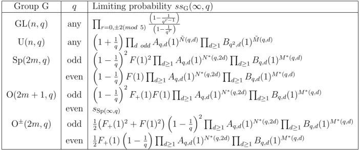
In this subsection let ssG(∞, q) denote the limiting probability of semisimple

matrices as n → ∞. We give the Table (2.7) of probabilities from ([7]). In this table results are expressed in terms of the following quantities

Aq,d(1) = µ 1 − 1 qd ¶ Ã 1 +X m≥1 1 |U(m, qd_)| ! , Bq,d(1) = µ 1 − 1 qd ¶ Ã 1 +X m≥1 1 |GL(m, qd_)| ! , F+(1) = 1 + X m≥1 µ 1 |O−_{(m, q)|} + 1 |O+_{(m, q)|} ¶ , F (1) = 1 +X m≥1 1 |Sp(m, q)|

In Table (2.8) we quote the lower and upper bounds for the limiting probability ssG(∞, q) from ([7]). The reader can also find convergence rates for the limiting

(35)

Group G q Limiting probability ssG(∞, q)

GL(n, q) any Q_{r=0,±2(mod 5)} ³ 1−_qr−11 ´ (1−_qr1 ) U(n, q) any ³ 1 + 1 q ´ Q d oddAq,d(1) ˜ N (q,d)Q d≥1Bq2_,d(1)M (q,d)˜ Sp(2m, q) odd ³ 1 −1 q ´₂ F (1)2Q d≥1Aq,d(1)N ∗_(q,2d)Q d≥1Bq,d(1)M ∗_(q,d) even ³ 1 −1 q ´ F (1)Q_d≥1Aq,d(1)N ∗_(q,2d)Q d≥1Bq,d(1)M ∗_(q,d) O(2m + 1, q) odd ³1 −1 q ´₂ F+(1)F (1) Q d≥1Aq,d(1)N ∗_(q,2d)Q d≥1Bq,d(1)M ∗_(q,d) even sSp(∞,q) O±_{(2m, q)} _odd 1 2 ¡ F+(1)2+ F (1)2 ¢ ³ 1 − 1 q ´₂_Q d≥1Aq,d(1)N ∗_(q,2d)Q d≥1Bq,d(1)M ∗_(q,d) even 1 2F+(1) ³ 1 −1 q ´ Q d≥1Aq,d(1)N ∗_(q,2d)Q d≥1Bq,d(1)M ∗_(q,d)

Table 2.7: Semisimple matrix limiting probabilities.

Group G q ssG(∞, q) lower bound ssG(∞, q) upper bound

GL(n, q) any 1 − q−1_{+ q}−3_{− 2q}−4 _{1 − q}−1_{+ q}−3 U(n, q) any 1 − q−1_{− q}−3_{− 2q}−4 _{1 − q}−1_{− q}−3_{+ 3q}−4 2 0.4698 0.4724 3 0.6498 0.6501 Sp(2m, q) odd 1 − 3q−1_{+ 5q}−2_{− 7q}−3_{+ 6q}−4 _{1 − 3q}−1_{+ 5q}−2_{− 7q}−3_{+ 13q}−4 even 1 − 2q−1_{+ 2q}−2_{− 2q}−3_{+ q}−4 _{1 − 2q}−1_{+ 2q}−2_{− 2q}−3_{+ 5q}−4 2 0.3476 0.3481 3 0.3819 0.3821 O(2m + 1, q) odd 1 − 2q−1_{+ 2q}−2_{− 2q}−3_{− 2q}−4 _{1 − 2q}−1_{+ 2q}−2_{− 2q}−3_{+ 7q}−4 3 0.5046 0.5053 O±_{(2m, q)} _odd _{1 − 2q}−1₊5 2q−2− 7 2q−3 1 − 2q−1+ 5 2q−2− 7 2q−3+ 21 2 q−4 3 0.5244 0.5252 even 1 2(1 − q−1− 3q−4) 12(1 − q−1+ 5q−4) 2 0.2513 0.2515

(36)

Chapter 3 Random Codes

This section is devoted to calculation of expectations and covariances between the coefficients of weight enumerator of random codes.

3.1 Expectations of Coefficients of Weight

Enu-merator

We will start with the moments of the random variable q−rk×n _{where r}

k×n is the

rank of a k×n matrix. The basic tool for evaluation of moments is the probability P (n, k, r) of the random k × n matrix to have rank r.

We need q-analogues [n]q of positive integers n and the q-factorials to express

this probability. Instead of the usual definition [n]q = (qn− 1)/(q − 1) we use the

following form

[n]q := qn− 1.

(37)

CHAPTER 3. RANDOM CODES 28

These functions extend the Binomial coefficients as follows [0]q! = 1, [n]_q! = [n]q[n − 1]q. . . [1]q, · n r ¸ q = [n]q! [r]q![n − r]q! . (3.1)

The quantum Binomial coefficient in Eq. (3.1) gives the number of r dimensional subspaces of an n dimensional linear space over Fq. Cardinality of the group

GL(k, q) is given by the factorial

|GL(k, q)| = qk(k−1)2 [k]_q! (3.2)

In the following part, we drop the subscript q in the notation. We will need two classical formulas in the sequel

q-Binomial Theorem (Commutative) Y 0≤j<d (1 − qjt) = X 0≤i≤d (−1)iqi(i−1)2 · d i ¸ ti, (3.3)

q-Binomial Theorem (Noncommutative) (x + y)d= X 0≤i≤d · d i ¸ xiyd−i, (3.4)

where the power on the left hand side is noncommutative in x and y. The power is to be expanded so that every monomial is in the form xi_yj _{by the relation yx=qxy.}

Note that the q-Binomial identities are expressed in q-Binomial coefficients and our convention on [n]q doesn’t change them. See ([12]) for the theory of the

subject and proofs of the items above.

Proposition 3.1 The probability P (n, k, r) of a k × n matrix to have rank r is given by P (n, k, r) = q−kn+r(r−1)₂ [n]! [n − r]! [k]! [k − r]! 1 [r]!. (3.5)

(38)

In the next theorem we will use the following simple lemma. Lemma 3.2 [k]! [k − d]! = q −d(d−1)₂ X 0≤i≤d (−1)i_qi(i−1)₂ · d i ¸ qk(d−i) _(3.6) Proof. [k]! [k − d]! = Y 0≤i<d (qk−i_{− 1) = q}kd−d(d−1)₂ Y 0≤i<d (1 − qi−k₎

When we replace the last product with the corresponding sum by Eq. (3.3) we get the result.

The following theorem gives the moments of the rank function of a random matrix.

Theorem 3.3 The sth _{moment µ}

s(q−rk×n) of the rank function q−rk×n is given by

µs(q−rk×n) = q−kn X 0≤r≤k qr(n−s) · k r ¸ Y 0≤i<r (1 − q−n+i), (3.7) µs(q−rk×n) = Y 0≤i<k (x + y − q−n−s+i₎ ¯ ¯ ¯ ¯ ¯ x=q−n_,y=q−s , (3.8)

where the product in the second formula is noncommutative in x and y. Ev-ery term should be put in the form xi_yj _{before substituting q}−n _{and q}−s _using

the commutation rule yx = qxy. Moment µs(q−rk×n) is symmetric in n and k.

Furthermore if s is a nonnegative integer then the formula is also symmetric in s.

(39)

Proof. We use the formula in Equation (3.5) for probability. µs(q−rk×n) = X r q−rs_{P (n, k, r)} = X r q−kn+r(r−1)₂ −rs [k]! [k − r]![r]! [n]! [n − r]! (3.9) = Eq.(3.6) q−kn X r,i q−rs · k r ¸ (−1)iqi(i−1)2 · r i ¸ qn(r−i) (3.10) = q−knX r qr(n−s) · k r ¸ Y 0≤i<r (1 − q−n+i₎ (3.11) To get the second formula of moments we proceed from Equation (3.10) as follows

µs(q−rk×n) = q−kn X r q−rs · k r ¸ X i (−1)i_qi(i−1)₂ · r i ¸ (qn₎r−i = r→k−r q−kn X r,i q−s(k−r) · k r ¸ (−1)i_qi(i−1)₂ · k − r i ¸ qn(k−r−i) = X r,i (−1)iqi(i−1)2 · k i ¸ qi(−n−s) · k − i r ¸ (q−n)r(q−s)k−i−r = X i (−1)iq(i)(i−1)2 · k i ¸ (q−n−s)i(q−n+ q−s)k−i (3.12) The last equation follows from the noncommutative q-Binomial formula (Eq. (3.4)). Finally by the commutative q-Binomial formula given in Eq. (3.3) we get

µs(q−rk×n) =

Y

0≤i<k

(q−n+ q−s− q−n−s+i)

where we remind that the product is noncommutative. It should be expanded in x = q−n_{, y = q}−s _{so that every monomial is put in the form x}i_yj _{by the}

commutation relation yx = qxy and then substitute for x and y.

The probability formula P (n, k, r) is symmetric in n and k hence the same holds for the moment formulas. This can be proven by expanding [k]!/[k − r]! instead of [n]!/[n − r]! in Eq. (3.9). If s is nonnegative integer the formula is completely symmetric in n, k and s. This follows from the symmetry of the noncommutative q-Binomial formula (3.4).

(40)

Example 3.1 An easy calculation gives the expectation E and the second moment µ2 of q−rk×n as follows

E(q−rk×n_{) = q}−n_{+ q}−k_{− q}−n−k_, _(3.13)

µ2(q−rk×n) = q−2n+ q−2k+ q−2n−2k+1+ q−n−k(q + 1)(1 − q−n− q−k). (3.14)

The following examples give the expectations of coefficients of weight enumer-ators of the random codes C and C⊥_{. In the following example and henceforth}

C is an [n, k] code given by a k × n random generator matrix.

Example 3.2 Expectation of weight enumerator of the random code C is given by E(WC(t)) = X i E(Ai)tn−i = tn+ (qk_{− 1)} qn (t + q − 1) n_. _(3.15)

Let G be a random k × n matrix and let C be the code with generator matrix G. Weight enumerator WC(t) is expressed via rank function by

WC(t) =

X

I⊂{1,2,...n}

qk−rI(t − 1)|I|,

where rI is rank of the column submatrix spanned by the column set I.

Expec-tation of the weight enumerator is given by E(WC(t)) =

X

I⊂{1,2,...n}

qk_E(q−rI_{)(t − 1)}|I|_.

The result follows when we substitute E(q−rI_{) = E(q}−rk×|I|_{) given by Equation}

(3.13).

We will obtain an analogous result for the random code C⊥ _{by Mac-Williams}

duality ([19]) W_C⊥(1 + t) = q−ktnW_C ³ 1 + q t ´ . (3.16)

Recall that C⊥ _{is considered to be an [n, n − k] code given by a random k × n}

parity check matrix.

Example 3.3 Expectation of weight enumerator of the random code C⊥ _{is given}

by E W_C⊥(t) = X i E(A⊥ i )tn−i = q−k((t + q − 1)n+ (qk− 1)tn). (3.17)

(41)

Let G be the random k × n parity check matrix of C⊥_{. We know expectation}

of weight enumerator of the code C which assumes G as its generator matrix (Example 3.2). Taking expectations of both sides of Eq. (3.16) and using Eq. (3.15) we obtain the assertion.

Expectations and the second moments of the code weights are not new results. One can find them in ([9, page 10]) and ([1, page 44]) for example.

3.2 Covariances Between the Coefficients of

Weight Enumerators

We will obtain the covariances between the coefficients of weight enumerators from the covariance of rank functions. The covariance between two rank functions is given by

cov(q−rI, q−rJ) = E(q−rI−rJ) − E(q−rI)E(q−rJ). (3.18) The new ingredient E(q−rI−rJ_{) requires the joint probability P (r}

I, rJ) of ranks

of sub-matrices GI and GJ spanned by the column sets I and J respectively. In

order to express P (rI, rJ) we need an auxiliary function. Let G be a k × n matrix

and let M fixed columns of G span a matrix of rank m. Denote by P (n, k, M, m, r) the probability that G has rank r.

Lemma 3.4

P (n, k, M, m, r) = P (n − M, k − m, r − m). (3.19) Proof. Let V0 be the column space of given M vectors. We have to find n − M

column vectors of rank r − m in the space Fk

q/V0 and then lift them up to Fkq. So

the number N(n, k, M, m, r) of complementary matrices is given by N(n, k, M, m, r) = q(n−M )(k−m)_{P (n − M, k − m, r − m)q}(n−M )m_.

(42)

The following proposition gives the moments of this partial probability func-tion.

Proposition 3.5 Moments of the partial rank function is given by X r q−rsP (n, k, r − m) = q−smµs(q−rk×n) (3.20) = q−sm−kn X 0≤r≤k qr(n−s) · k r ¸ Y 0≤i<r (1 − q−n+i_)(3.21) = q−sm Y 0≤i<k (q−n+ q−s− q−n−s+i) (3.22) where in the last formula the product is noncommutative in the variables x = q−n

and y = q−s_{. Moment formula is symmetric in n and k. Moreover when m = 0}

and s is a nonnegative integer the formula is completely symmetric in n, k and s. Proof. Proof of this proposition repeats the same steps as Theorem (3.3) so we skip the proof.

Theorem 3.6 Let G be a random k × n matrix, I, J ⊂ {1, 2, . . . , n} be two sets of columns. Then covariance between the rank functions q−rI _{and q}−rJ _{is given}

by

cov(q−rI_{, q}−rJ_{) =} (q − 1)(qk− 1)(q|I∩J|− 1)

q2k+|I|+|J| . (3.23)

Proof. Covariance is given by

cov(q−rI, q−rJ) = E(q−rI−rJ) − E(q−rI)E(q−rJ). (3.24) So we need the expectation of q−rI−rJ_{, hence the joint probability P (r}

I, rJ) of

ranks rI and rJ. This probability is given by the following sum

P (rI, rJ) =

X

r

P (IJ, k, r)P (I, k, IJ, r, rI)P (J, k, IJ, r, rJ),

where IJ is the shortcut notation for |I ∩ J|. The sum runs over the rank of the intersection. We extend the intersection to the sets I and J with ranks rI and

rJ. Substituting for the auxiliary probabilities by Equation (3.19) we get

E(q−rI−rJ_{) =} X r,rI,rJ

q−rI−rJ_{P (IJ, k, r)P ( ¯¯}_{I, k − r, r}

(43)

where ¯¯I = |I \ J| and ¯¯J = |J \ I|. We can sum up over rI and rJ by Equations

(3.13) and (3.20) E(q−rI−rJ_{) =}X

r

P (IJ, k, r)¡q−k_{(1 − q}− ¯I¯_{) + q}−r− ¯I¯¢¡_q−k_{(1 − q}− ¯J¯_{) + q}−r− ¯J¯¢_.

Finally summation over r gives

E(q−rI−rJ) = q−2k(1 − q− ¯I¯)(1 − q− ¯J¯) + q− ¯I− ¯¯ J¯µ2(q−rk×IJ) +

³

q− ¯I−k¯ (1 − q− ¯J¯) +q− ¯J−k¯ _{(1 − q}− ¯I¯₎´_E(q−rk×IJ_).

We have expressed E(q−rI−rJ_{) in terms of the first and the second moments of the}

rank function and they are given by Equations (3.13) and (3.14). If we substitute this with the product E(q−rI_)E(q−rJ_{) in Equation (3.24) we get the assertion.}

While the covariances between the rank functions of column submatrices are enough for code theoretical purposes the same question about arbitrary subma-trices is still an interesting problem. Let G be a random k × n matrix. Let I ⊂ {1, 2, . . . , n} be a column set and L ⊂ {1, 2, . . . , k} be a row set. We denote by rLI rank of the submatrix spanned by the rows in L and the columns in I.

Conjecture 3.7 Covariance between the rank functions q−rLI_{, q}−rM J _{of two}

sub-matrices is given by

cov(q−rLI, q−rM J) = (q − 1)(q

|I∩J|_{− 1)(q}|L∩M |_{− 1)}

q|I|+|J|+|L|+|M | .

Before we proceed with the covariance of code weights, we need the following lemma. Lemma 3.8 Let Sij = X I,J⊂{1,2,...n} |I|=i,|J|=j q|I∩J|. (3.25)

We have the following generating function for Sij

X

i,j

Random codes and matrices

RANDOM CODES AND MATRICES

a dissertation submitted to

the department of mathematics

and the institute of engineering and science

of bilkent university

in partial fulfillment of the requirements

for the degree of

doctor of philosophy

By

˙Ibrahim ¨Ozen

ABSTRACT

RANDOM CODES AND MATRICES

¨

OZET

RASTSAL KODLAR VE MATR˙ISLER

Acknowledgement

Contents

Chapter 1

Introduction

1.1

A Brief Overview of Random Matrices

1.1.1

Complex Random Matrices

1.1.2

Random matrices over finite fields

1.2

Random codes

1.3

Statement of Results

Chapter 2

Known Results Over Finite

Fields

2.1

Results for Mat(n, q) and GL(n, q)

2.1.1

Similarity Classes

2.1.2

Cycle Indices

2.2

Results for Other Classical Groups

2.2.1

Separable Matrices

2.2.2

Cyclic and Regular Matrices

2.2.3

Semisimple Matrices

Chapter 3

Random Codes

3.1

Expectations of Coefficients of Weight

Enu-merator

3.2

Covariances Between the Coefficients of

Weight Enumerators