Optimization of gendarmerie posts' main supply roads via regional ring transportation system

OPTIMIZATION OF GENDARMERIE POSTS’

MAIN SUPPLY ROADS VIA REGIONAL RING

TRANSPORTATION SYSTEM

A THESIS

SUBMITTED TO THE DEPARTMENT OF INDUSTRIAL

ENGINEERING

AND THE INSTITUTE OF ENGINEERING AND SCIENCES

OF BILKENT UNIVERSITY

IN PARTIAL FULFILMENT OF THE REQUIREMENTS

FOR THE DEGREE OF

MASTER OF SCIENCE

By

Yunus Emre KARAMANOĞLU

JULY, 2004

I certify that I have read this thesis and in my opinion it is fully adequate, in scope and in quality, as a thesis for the degree of Master of Science.

Assoc. Prof. Osman Oğuz (Principal Advisor)

I certify that I have read this thesis and in my opinion it is fully adequate, in scope and in quality, as a thesis for the degree of Master of Science.

Prof. Mustafa Ç. Pınar

I certify that I have read this thesis and in my opinion it is fully adequate, in scope and in quality, as a thesis for the degree of Master of Science.

Asst. Prof. Oya Ekin Karaşan

Approved for the Institute of Engineering and Sciences

Prof. Mehmet Baray

ABSTRACT

OPTIMIZATION OF GENDARMERIE POSTS’

MAIN SUPPLY ROADS VIA REGIONAL RING

TRANSPORTATION SYSTEM

Yunus Emre KARAMANOĞLU

M.S in Industrial Engineering

Advisor: Assoc. Prof. Osman OĞUZ

JULY 2004

The aim of this study is to find the optimum distances traveled by the vehicles distributing goods to the military units, belonging to a command center, in one day and the appropriate fleet types and sizes for each Command Center. We examine the differences in the total distances traveled by the vehicles when the types and number of the vehicles are changed in the fleet. A mixed integer programming model is proposed, and for the implementation of

the model, optimization modeling software GAMS is used. The proposed model is obtained from the current system elements and shows the differences between the current distribution system and the solution of the proposed model. How the total distances are affected when distribution is made from one center is investigated, and ideal main supply routes, ideal sequences of supply plans, and fleet sizes are proposed.

Keywords: Mixed integer Programming, Fleet Size and Capacitated Vehicle Routing, Regional Ring Transportation System.

ÖZET

JANDARMA KARAKOLLARININ ANA İKMAL

GÜZERGAHLARININ BÖLGESEL RİNG TAŞIMA

SİSTEMİYLE OPTİMİZASYONU

Yunus Emre KARAMANOĞLU

Endüstri Mühendisliği Bölümü Yüksek Lisans

Tez Yöneticisi: Doç. Dr. Osman OĞUZ

TEMMUZ 2004

Bu çalışmada, askeri birliklerin en küçük birlik seviyesine kadar yapılmakta olan ikmallerinin aynı gün içerisinde yapılması için gereken araç filo sayısını bulmak ve bu araçların katettikleri mesafeleri optimum seviyeye indirmek amaçlanmıştır. Farklı araç, tip ve sayıları kullanıldığında toplam mesafede oluşan farklılıklar incelenmiştir. Tamsayılı programlama modeli önerilmiş ve bu modelin uygulanması için GAMS yazılımı kullanılmıştır. Model hali hazırda bulunan sistemle belirlenmiş olup, şu anki sistemle önerilen sistem arasındaki farkları ortaya koymaktadır. Toplam dağıtım mesafelerinin merkezi sistem kullanıldığında nasıl etkilendiği sorusuna yanıt bulunmaya çalışılmış ve ideal güzergahlar tesbit edilmiş ve en uygun ikmal planlama sırası önerilmiştir.

Anahtar Kelimeler: Tamsayılı Programlama, Filo Hacmi ve Kapasite Sınırlı Araç Güzergahı Bulma, Bölgesel Ring Taşıma Sistemi.

ACKNOWLEDGEMENT

I am indebted to Assoc. Prof. Osman OĞUZ for his valuable guidance, understanding, and above all for enthusiasm which he inspired on me during this thesis.

I am also indebted to the readers Prof. Mustafa Ç. PINAR and Asst. Prof. Oya Ekin KARAŞAN for showing keen interest to the subject matter and accepting to read and review this thesis.

I would like to thank Captain İbrahim CAN, First Lit. Nejdet KARACA, First Lit. Ünal AKMEŞE for their support.

I am very thankful to M. Rasim KILINÇ, M. Oğuz ATAN, Ayşegül ALTIN, Zümbül BULUT, Salih ÖZTOP, Damla and Güneş ERDOĞAN for their support, assistance and friendship during the graduate study.

I would like to thank all Industrial Engineering Faculty, staff and my friends for their assistance and support during the graduate study.

I would like to thank The General Command of Gendarmerie for giving me the opportunity to continue my education in Bilkent University.

Finally I am very thankful to my mother, my father and my sister for their support, tolerance and patience.

CONTENTS

List of Figures IX

List of Tables X

English-Turkish Meanings of Some Military Terms XI

1. INTRODUCTION

1.1. Regional Ring Transportation System (RRTS) 2 1.1.1. Current Distribution System 3

1.1.1.a. Distribution of Deliveries to Companies and Out-posts 3

1.1.1.b. Picking-Up the Items from Company Points and Out-posts 4

1.1.2. Proposed Distribution System

2. LITERATURE REVIEW

2.1. The Traveling Salesman Problem (TSP, M-TSP) 9

2.1.1. TSP and M-TSP Optimal Approaches 11

2.1.2. TSP and M-TSP Heuristic Solution Methods 14

2.1.2.1. Tour Construction Procedures 14

2.1.2.1.1. Nearest Neighbor Procedures 14

2.1.2.1.2. Clarke and Wright Savings 15

2.1.2.1.3. Insertion Procedure 15

2.1.2.1.4. Minimal Spanning Tree Procedure 16

2.1.2.1.5. Christofides’ Heuristic 17

2.1.2.1.6. Nearest Merger 17

2.1.2.2. Tour Improvement Procedures 18

2.1.2.3. TSP and M-TSP Composite Procedures 19

2.1.2.4. Akl’s Directed TSP Approach 20

2.1. The Vehicle Routing Problems 20

2.2.1. Solution Strategies of VRP’s 21

2.2.1.1. Saving or Insertion Procedures 22

2.2.1.2. Cluster First-Route Second 22

2.2.1.3. Route First-Cluster Second 23

2.2.1.4. Improvement or Exchange Procedure 23

2.2.1.5. Mathematical Programming Approaches 23

2.2.1.6. Interactive Optimization 24

2.3.2. Solution Techniques for Single Depot VRP’s 25

2.3.2.1. The Savings Algorithm 25

2.3.2.2. The Sweep Approach 25

2.3.2.3. A Penalty Algorithm 26

2.3.2.4. M-Tour Approach 26

2.3.2.5. A Generalized Assignment Heuristic 26

2.3. The Fleet Size and Mix Vehicle Routing Problems 26

3. The PROBLEM and FORMULATION

3.1. Data Lists 32

3.1.1. Points 33

3.1.2. Vehicles 33

3.1.3. Materials 34

3.2. Assumptions for the Problem Formulation 34

3.2.1. Security of the Roads is not considered 34

3.2.2. All demands (Delivery/Pick-up) of the points must be satisfied 34

3.2.3. Vehicle speeds are fixed 35

3.2.4. The load and unload times are fixed 35

3.2.5. Time windows are fixed 35

3.2.6. The cost of vehicles in fleet is considered to be same 35 3.2.7. The utilization rate of the vehicle in fleet is important 35

3.2.8. Fleet sizes for each regiment center is considered to be same 36 3.2.9. Mobile posts are not considered 36

3.3. Formulation 36

3.3.1. Notation 36

3.3.2. Initial Data and Parameters 37

3.3.3. Variables 37

3.3.4. Objective Function and Formulation 38

3.3.5. Explanation of the Formulation 40

4. COMPUTATIONAL RESULTS

4.1. Results 47

4.1.1. Regiment Center-A 48

4.1.2. Regiment Center-B 49

4.1.3. Regiment Center-C 49

4.1.4. Comparison of the Distribution Systems in Distance 50 4.1.5. Comparison of the Distribution Systems in Cost 52 4.1.6. General Comparison of the Systems in Distance and Cost 53

5. CONCLUSION

5.1. Future Research Topics 56

BIBLIOGRAPHY 58

APPENDIX 66

LIST OF FIGURES

Figure 1.2. Current System 5

Figure 1.3. Proposed System 7

Figure 2.2.1.1. Two Subtours on a graph of 6 nodes 11

Figure 2.3.2.1. Savings Algorithm 25

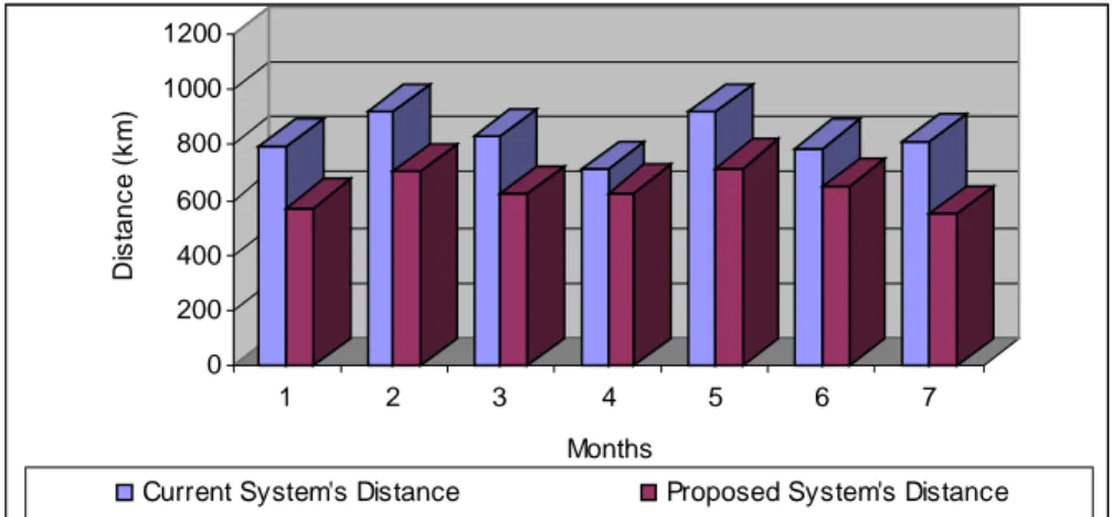
Figure 4.1. Comparison of the Current System with the Proposed System in

Distance for months in Command A 51

Figure 4.2. Comparison of the Current System with the Proposed System in

Distance for months in Command B 51

Figure 4.3. Comparison of the Current System with the Proposed System in

Distance for months in Command C 51

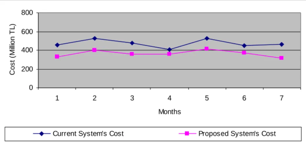
Figure 4.4. Comparison of the Current System with the Proposed System in

Cost for months in Command A 52

Figure 4.5. Comparison of the Current System with the Proposed System in

Cost for months in Command B 52

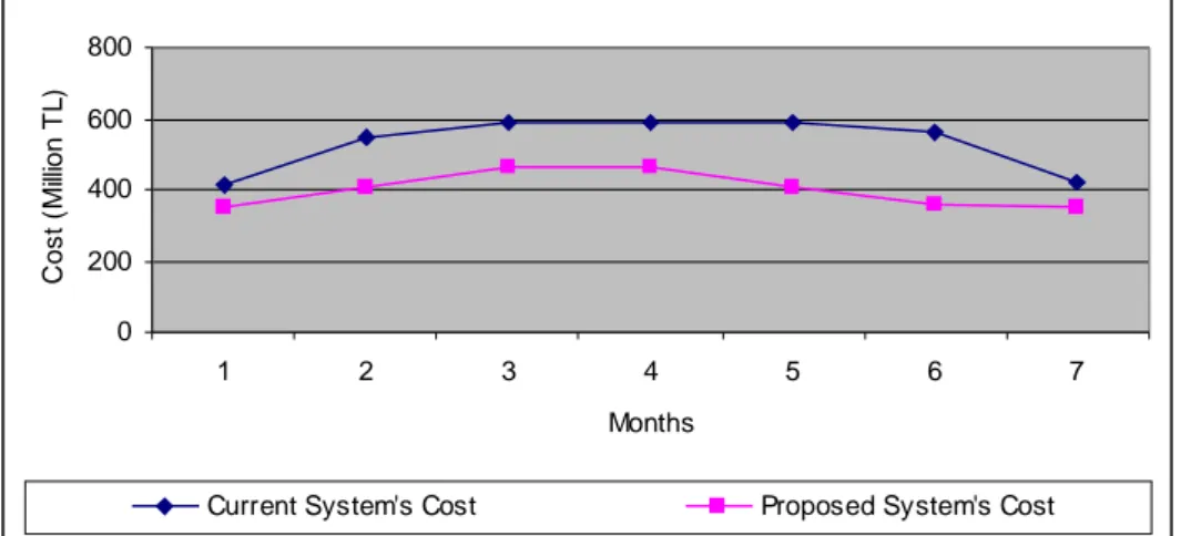
Figure 4.6. Comparison of the Current System with the Proposed System in

Cost for months in Command C 53

Figure 4.7. General Comparison of the Current System with the Proposed

System in Average Distances for months in selected Command 54

Figure 4.8. General Comparison of the Current System with the Proposed

LIST OF TABLES

Table 1.1. Demanding Points of the Sample Problem 7

Table 3.1. Capacities of the selected vehicles (in 1000 kgs) 34

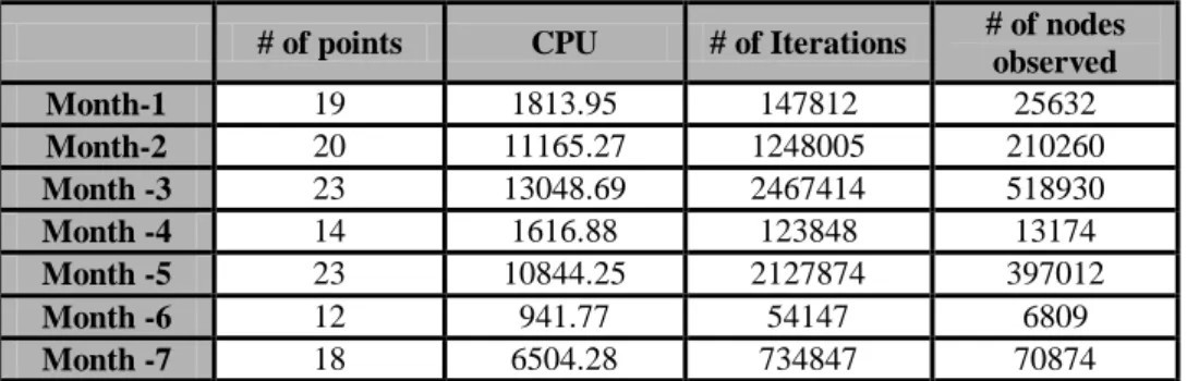
Table 4.1. Required CPU times, number of iterations and number of nodes

observed for Command-A 45

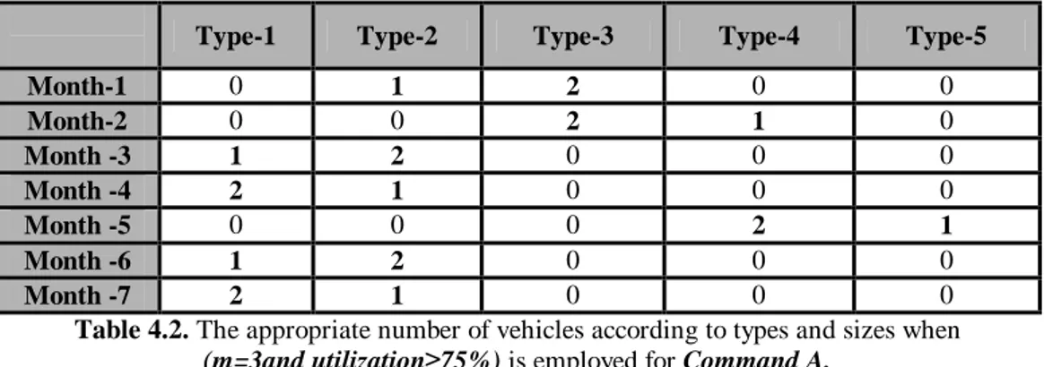
Table 4.2. The appropriate number of vehicles according to types and sizes

when (m=3and utilization≥75%) is employed for Command-A 45

Table 4.3. Required CPU times, number of iterations and number of nodes

observed for Command-B 46

Table 4.4. Required CPU times, number of iterations and number of nodes

observed for Command-C 46

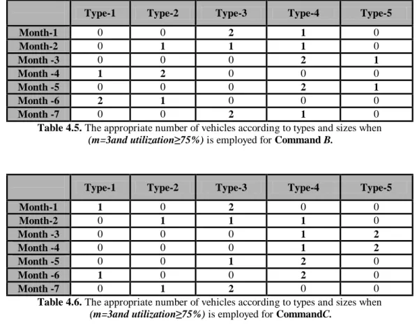
Table 4.5. The appropriate number of vehicles according to types and sizes

when (m=3and utilization≥75%) is employed for Command-B 47

Table 4.6. The appropriate number of vehicles according to types and sizes

when (m=3and utilization≥75%) is employed for Command-C 47

Table 4.7. Total distances and costs for distribution in Command-A 48

Table 4.8. Total distances and costs for distribution in Command-B 49

Table 4.9. Total distances and costs for distribution in Command-C 50

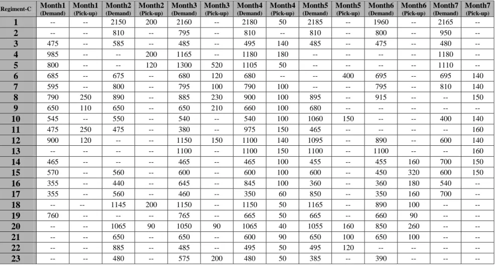
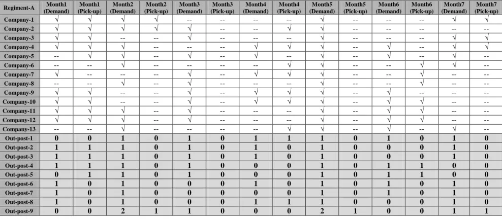
Table A.1.Delivery/Pick-up amounts (kg) of the points in Regiment Center A 66

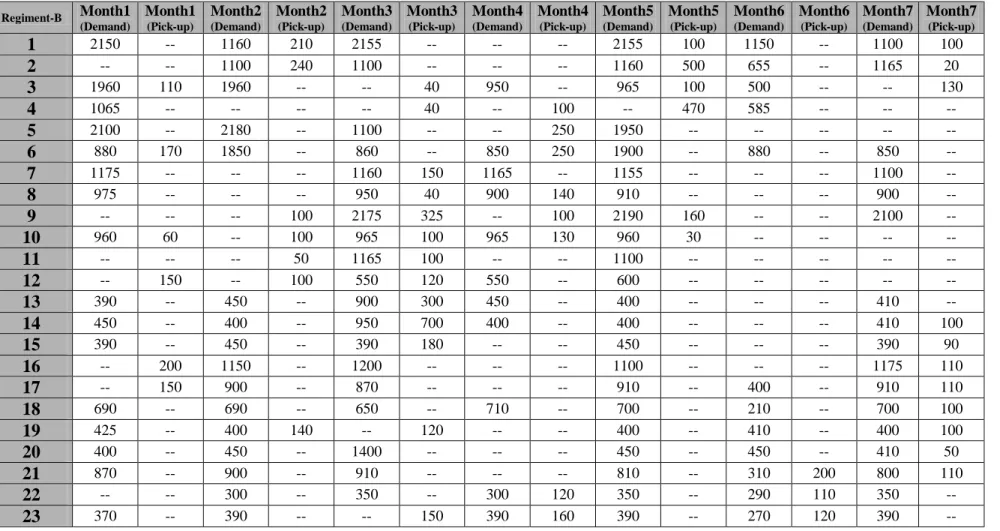
Table A.2.Delivery/Pick-up amounts (kg) of the points in Regiment Center B 67

Table A.3. Delivery/Pick-up amounts (kg) of the points in Regiment Center C 68

Table A.4. Records the vehicles in Regiment Center A 69

Table A.5. Records the vehicles in Regiment Center B 70

English-Turkish Meanings of Some Military Terms

Brigade: Tümen

Regiment: Alay

Regiment Center: Alay (İl) Merkezi

Company: Bölük

Company Center: Bölük (İlçe) Merkezi

Out-post: Dış Karakol

Out-post Point: Karakol (Kasaba) Merkezi

Gendarmerie Post: Jandarma Karakolu

CHAPTER 1

INTRODUCTION

In the battlefield, one of the most crucial factors that a commander must consider is the logistics system of the military units. The army may lose the war, because of a poor logistics system. Turkish Armed Forces has implemented many modifications in its structure to catch up with technological development in recent years. In context of these modifications, Armed Forces have started projects with the aim of improving the distribution system of the units.

The word logistics comes from the Greek word “λογιστικος”, meaning skilled in calculation. Further, the dictionary defines logistics as the branch of military service having to do with moving, supplying and quartering troops. These descriptions imply that logistics involves the care and feeding of combat forces and the necessary measures to provide this support.

Lessons taken from the recent history about military logistics are very important. We can say that military logistics is the art and science of equipping and supplying armies. If military logistics is done well, it is a significant combat multiplier. There is an old saying: “For want of the nail a shoe was lost, for want of a shoe the horse was lost...Ultimately, the war was lost for the want of a nail.” Logistics is that important to war fighting. For this reason; supplying the demands of specially dispersed points is a critical issue for command.

The demands of points must be satisfied in very short time limits because the lateness in logistics may prevent the execution of the given duties to the units. All of the Commands use highway transportation. (In some cases, airway and railway transportations are also being used) A modern transportation concept is based on the principle of delivering goods from an address to demanding address or picking up goods from demanding address to another

address. Ring transportation has been in preference among the transportation systems in military since it is more economical and secure.

Ring transportation system is composed of Central Ring Transportation System (CRTS) and Regional Ring Transportation System (RRTS). Since RRTS meets transportation demands inside of Brigades’ and Regiments’ own responsibility areas, our distribution system can be thought as a Regional Ring Transportation System.

This study begins with the problem definition of the current system and proposed system. In Chapter 2, we present the types of vehicle routing problems and related literature. This chapter covers traveling salesman problem (TSP), single-multiple vehicle routing problem(VRP), delivery-pickup problem, time dependent vehicle routing problems, fleet size and mix vehicle routing problem (FSMVRP) and application of areas of different routing problems.

We present the constructions of the model in Chapter 3. We firstly state our assumptions, and then present the indices, variables and constraints that belong to our formulation. In Chapter 4, we present the computational results obtained from our model and the differences between the current and proposed system. In Chapter 4, we also present the suitable vehicle types and sizes for each month. In Chapter 5, we give a summary of our research and conclude the study along with suggestions for future research directions.

1.1 Regional Ring Transportation System

RRTS’s mission is to deliver items from Regiment Center to Companies and to pick up items from Companies to bring to Regiment Center. Delivering to points is named as provision. The type of provision being used is explained in Section 1.1.1. Pick ups depend on the demand points requiring items in their own areas be sent to Main Repair Factories in the Main Center through

Regiment Center, i.e., to send a defective machine, weapon and ammunition for repair. Regiment Centers use this distribution system.

1.1.1. Current Distribution System

1.1.1. a. Distribution of Deliveries to Companies and Out-Posts

In current RRTS, fixed routes are performed according to the responsibility area of the Regiment Centers. The number of the fixed routes may change according to the number of the company points located in that responsibility zone. All demands (pick-up/delivery) must be satisfied in one-day period following the vehicles’ departure. RRTS delivers only to the Company Points and Out-posts that are located in the responsibility area of the Company Points in consideration; take their demands from their Company Points. This means that the vehicles of the Out-posts make extra mileages and this effects vehicle utilization. (In our study and in our tables, we used the term, “Total Distance”; which includes Fixed Routes between Company Points and Regiment Center; and distances traveled by the vehicles of the Out-posts. “Total Distance = Fixed Route + Distances traveled by the vehicles of Out-posts”. Distances between Company Points and Out-posts are considered if the Out-post has demand/pick-up).

RRTS delivers to the company points in two occasions: First, points can request any item from Regiment Center at any time. Then, RRTS delivers to these points. Secondly, Points are visited periodically. Regiment Center knows when to deliver to the company points without being informed. The word “delivery demand” will stand for two occasions in the following parts of our study.

In our study, we select three Regiment Centers; Regiment Center A has totally 22 points (13 Company Points and 9 Out-post Points), Regiment Center

B has 23 points (15 Company Points and 8 Out-post Points) and Regiment Center C has totally 23 points (14 Company Points and 9 Out-post Points).

Out-posts are located according to responsibility area of the Company Points, for this reason; a company may have more than one out-post in its responsibility area. There are also Companies that have no Out-post in their responsibility areas.

1.1.1. b. Picking-Up the Items from Company Points and Out-Posts

RRTS also picks up items from the points. The points make “pick-up demand” when they have any item to send to Regiment Center or to the factories.

In the current system, points do not inform Regiment Center about their pick-up demands since points are being visited periodically. The Pick-Up demands of the Out-posts are not taken from their original locations. These units bring their pick-up demands to their Company Centers’ locations, and RRTS pick-ups these items from Company Centers. This effects the vehicle utilization and creates problems in transportation.

Each vehicle is assigned to a tour and then loaded after Regiment Center have gotten information of delivery demands according to the delivery demand quantities of points on vehicles’ routes. The vehicle fleet loaded with delivery demands come back to Center with the load that they picked up from the pick-up demanding points after completing the routes.

In the current system, vehicle utilizations are not considered either. Some of the vehicles return to their locations empty, and some of the vehicles, especially the vehicles of the out-posts, go to their company points empty, take their demand and return back. This effects vehicle utilization and vehicles travel unnecessary distances and consequently the cost of a distribution in the area of a regiment center increases.

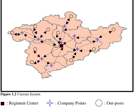
When we think that Gendarmerie is responsible for security and public order over 91% of Turkey, and also when we think that there are 81 Gendarmerie Regiment Points, 901 Gendarmerie Company Points and 2581 Out-posts in Turkey (valid for year 2003); we can easily see the economical significance of the problem (Cost of the distribution system is approximately $800,000 per year). For this reason, an appropriate distribution system for these regiment centers is very important for our military units.

Figure 1.2 shows the current distribution system:

Figure 1.2Current System

: Regiment Center : Company Points : Out-posts : Fixed Routes between Regiment and Companies

: Routes between Companies and Out-posts

This application brings fixed travel distance and fixed cost for each time since fixed routes are performed even if some points on the routes have zero demand or pick-up, and some of the out-post points are visited twice in this system.

It is clear that this fixed travel distance (cost) includes unnecessary distance (cost) due to ignoring non-demanding points and extra utilization of the out-post vehicles.

1.1.2. Proposed Distribution System

In all habited parts of our country, there are companies or out-post points ready to sustain public security and order. The distribution system of these units is very important because, a problem in the distribution system may cause an important difficulty in performing the given duties. Our aim is to develop a mathematical programming model to provide a better operational system for RRTS. In our mathematical model, only demanding points are visited including out-posts on the route by the appropriate vehicle types and sizes. The types and sizes of the vehicles that are to be used in the fleet are very important because of their utilization rates. In all of the areas as in the military, for different types of systems there exist preset limits and these limits determine the performance and profit of the system under consideration. For this reason, in our study, we use a utilization limit for the vehicles in our fleet. The vehicles having a utilization rate under a limit are not to be considered.

The fleets of The Regiment Centers are to be formed by mid-class vehicles because of the road characteristics of Turkey. This will be clearer when we present the assumptions used in our study. In our model, the vehicles will visit all of the demanding points on their routes and they will not consider whether the visiting point is a company point or out-post. By the help of this procedure the vehicles of the out-posts will not be used and will not make extra and unnecessary mileage.

To give an example, let us assume that in a selected Regiment Center that have nineteen points including both Companies and Out-posts (9 Company Points and 10 Out-post Points), only ten points have demands (pick-up/delivery) and these points inform Regiment Center about their demand

quantities. We only aim to show the improvement in travel distance (cost) in this part. Table 1.1 shows these demanding (pick-up/delivery) points:

1 2 3 4 5 6 7 8 9 10 11 12 13 14 15 16 17 18 19

Delivery √ √ √ √ √

Pick-up √ √ √ √ √ √ √ √ √ Table 1.1 Demanding Points of the Sample Problem

Figure 1.3Proposed System

: Regiment Center : Company Points : Out-posts

Optimal solution of our Mixed-Integer Programming Model is shown in Figure 1.3. The points in black are demanding points.

Appropriate vehicle fleet visits only demanding customers. This application enables us to get rid of unnecessary distance (cost) and unnecessary utilization of the vehicles of out-posts. It can easily be seen that we can determine the vehicle fleet size giving the optimal solution by considering the number of demanding points.

In this thesis, our goal is to investigate how the total distance (cost) is affected when the proposed system for RRTS (with the appropriate vehicle types and sizes) is employed. We have developed a mixed-integer programming model. The models determine which routes will be followed and assign demands (pick-up/delivery) to appropriate vehicle types and sizes. The objective of the models is to minimize distance, transportation costs and get rid of the extra mileages of the vehicles. The mixed-integer programming model is solved for a seven-month data.

CHAPTER 2

THE LITERATURE REVIEW

Vehicle Routing Problem is an important research area in industrial engineering and in operations research that encompasses a wide range of problems such as the delivery/pick-up of the items of the customers, time dependent delivery/pick-up problems, distribution of the goods of private firms to customer locations,…, etc.

The effective management of the vehicles belonging to a fleet gives rise to a variety of ‘Vehicle Routing Problems’ (VRP). The basic routing problem is easy to state. We are given a set of nodes or arcs to be served by a fleet of vehicles. There are no restrictions on when or the order in which these entities must be served. The problem is to construct a low-cost, feasible set of routes— one for each vehicle. A route is a sequence of locations that each vehicle must visit along with an indication of the service it provides.

The routing of vehicles is primarily a spatial problem. It is assumed that no temporal or other restrictions impact the routing decision except maximum route-length constraints. This is in contrast to scheduling problems, where the movement of each vehicle must be traced through both time and space.

Due to relatively unconstrained nature of these problems and their inherent complexity, they have challenged combinatorial analysts and operations researchers for many years.

2.1. The Traveling Salesman Problem (TSP, M-TSP)

The TSP is the problem of finding a route for a salesman such that total distance traveled or cost is minimized. In its most basic form, TSP is the problem of finding the shortest route in a given graph which starts and ends at

the same node, called origin, with all the other nodes visited exactly once. M-TSP is a generalized version of the well-known M-TSP that comes closer to accommodating real world problems where there is a need to account for more than one salesman (vehicle). Some basic routing problems are:

a. The Traveling Salesman Problem, b. The Chinese Postman Problem, c. The M-Traveling Salesman Problem,

d. The Single Depot, Multiple Vehicle, Node Routing Problem, e. The Multiple Depot, Multiple Vehicle, Node Routing Problem, f. The Single Depot, Multiple Vehicle, Node Routing Problem with stochastic demand

g. The Capacitated Chinese Postman Problem

Let G = [N, A, C] be a network defined with N the set of nodes (vertices), A the set of edges, and C = [cij] the matrix of costs. That is, cij is the

cost of moving or the distance from node i to node j. The traveling salesman problem requires the Hamiltonian cycle in G of minimal total cost. (A Hamiltonian cycle is a cycle passing through each node i∈N exactly once) Many interesting aspects of this problem have been discussed by Bellmore and Nemhauser (1974) and Christofides (1976a). Kirkpatrick et al. (1982) studied the connections between statistical mechanics and TSP.

Karp (1972) has shown that the traveling salesman problem (TSP) is NP-complete. Garey et al. (1976) and Papadimitriou (1977) have showed that it is NP-hard even when additional assumptions such as the triangle inequality (C is said to satisfy the triangle inequality if and only if cij + cjk ≥ cik for all i, j, k∈

N) or Euclidian distances are invoked.

Little et al. (1963), Held and Karp (1970), (1971), Miliotis (1976), Crowder and Padberg (1980) have proposed ingenious algorithms for the TSP.

Due to the difficulty of the TSP, many heuristic procedures have been developed. Rosenkrantz, Stearns, and Lewis (1977) have compared these heuristics analytically by studying worst-case behavior. Golden et al. (1980) has used some computational experimentation to compare the performance of these heuristics.

Stewart (1981) has described a number of new algorithms designed specifically to perform well on Euclidian problems.

2.1.1. TSP and M-TSP Optimal Approaches

Optimal approaches to the TSP are based on mathematical programming formulations. The TSP and M-TSP are generally formulated as integer linear programs based as follows. Let,

1, if edge ( , ) is in the tour 0, otherwise

ij

i j X = 



Xij is a 0-1 variable indicating whether or not a salesman goes directly

from node i to node j. Then we would like to find Xij which are to become 1,

i.e. finding the edges that salesman should go through, for the distance traveled or cost to be minimized. An assignment-based formulation of a problem selects the matrix X=( xij) of decision variables so that exactly one arc (i, j) emanates

from each node i and exactly one arc (i, j) is directed into each node j. This implies an assignment of each node to its successor node on the tour. The assignment requirements do not ensure that the matrix X corresponds to a tour. Instead, the assignment may result in subtours as shown in Figure 2.1.1.1:

2 3 4 5

1 6

To eliminate the possibility of subtours, some restrictions are imposed on the choices for arc selection matrix X. A typical formulation for TSP can be like the following one:

Minimize

∑∑

∑

∑

The set S can be any restrictions that prohibit subtour solutions satisfying the assignment constraints (2), (3), and (5). Such restrictions are called subtour-breaking constraints. Possible choices for S include:

(i) S={(xij):

∑∑

x 1 for every nonempty proper subset Q of N};

(ii)S={(xij):

∑∑

x 1 for every nonempty subset R of {2,3,..,n}};

(iii)S={(xij): yi - yj + n xij ≤ n-1 for 2≤ i≠j ≤n for some real numbers yi }.

In these notations, S contains nearly 2n subtour-breaking constraints in (i) and (ii) but only n2-3n+2 constraints in (iii). We can observe that the configuration in our Figure 2.1.1.1 satisfies constraints (2), (3), and (5), but not (4). That is, it does not represent a tour. The first set of subtour-breaking constraints (i) states that every proper subset Q of nodes must be connected to the other nodes in the network in the solution X. They prohibit the solution in Figure 2.1.1.1 when Q=(1,2,3). The second set of subtour-breaking constraints (ii) implies that the arcs selected in X contain no cycle, since a cycle on nodes R must contain‌‌‌‌ R arcs. It excludes the solution in our Figure 2.1.1.1 when R=(4,5,6). The third set of subtour-breaking constraints is more complicated.

Adding constraints (iii) for arcs 4-5, 5-6, and 6-4 in Figure 2.2.1.1 yields 3n≤3(n-1), a contraction. A similar contradiction arises whenever the matrix X contains a subtour solution. Thus, each set of constraints (i), (ii), and (iii) prohibits subtours.

The first Integer Linear Programming formulation (ILP) for the m-TSP was given by Miller, Tucker and Zemlin (MTZ) (1960). In the formulation of MTZ, the salesman turns back to the origin, denoted by 0, t times.

Minimize

∑ ∑

∑

∑

∑

{ }

The constraint (1) forces the salesman to turn back to the origin exactly t times. The constraints (2) and (3) are the usual degree constraints of an assignment problem. They proposed constraint (4) by using extra variable in order to reduce the number of exponentially growing subtours, which do not include the origin.

These constraints are generally called subtour elimination constraints (SEC). In constraint (4), p is the maximum number of nodes that a salesman is allowed to visit and ui are arbitrary real numbers.

In the following part, we present some heuristics solution approaches and exact solution methods from the literature:

2.1.2. TSP and M-TSP Heuristic Solution Methods

The heuristics, we examine from the existing literature, fall into three classes: Tour Construction Procedures, Tour Improvement Procedures and Composite Procedures. Tour Construction Procedures generate an approximately optimal tour from the distance matrix. Tour Improvement Procedures attempt to find a better tour given an initial tour. Composite Procedures construct a starting tour from one of the tour construction procedures and then attempt to find a better tour using one or more of the tour improvement procedures. Most of these procedures are described in the literature:

2.1.2.1. Tour Construction Procedures

2.1.2.1.1. Nearest Neighbor Procedure

Rosenkrantz, Stearns, Lewis (1977) have applied this procedure. The steps of the procedures are the following:

Step 1. Start with any node as the beginning of a path.

Step 2. Find the node closest to the last node added to the path. Add this node to the path.

Step 3. Repeat step 2 until all nodes are contained in the path. Then, join the first and last nodes.

Worst Case Behavior:





where lg denotes the algorithm to the base 2,

 

times, each time with a new node selected as the starting node. The best solution obtained can be listed as the answer. This strategy runs in an amount of time proportional to n3.

2.1.2.1.2. Clarke and Wright Savings

Clarke and Wright (1964) were the first to present this algorithm and Golden (1977b) has applied this procedure in his work. The procedure is the following:

Step 1. Select any node as the central depot that is denoted as node 1. Step 2. Compute savings sij = c1i + c1j - cij for i,j = 2,3,…,n.

Step 3. Order the savings from largest to smallest.

Step 4. Starting at the top of the savings list and moving downwards, from larger subtours by linking appropriate nodes i and j. Repeat until a tour is formed.

Worst Case Behavior: The worst-case behavior of this approach is known for both a sequential and concurrent version. Golden (1977a) has demonstrated that for a sequential version of this algorithm where at each step we select the best savings form the last node added to the subtour, the worst case ratio is bounded by a linear function in lg(n).

Ong (1981) has derived a similar result for the concurrent version.

The Clarke and Wright savings procedure requires on the order of n2lg(n) computations.

2.1.2.1.3. Insertion Procedure

Rosenkrantz, Stearns, and Lewis (1977) have applied this procedure in their paper. An insertion procedure takes a subtour on k nodes at iteration k and

attempts to determine which node (not already in the subtour) should join the subtour next (the selection step).

In the literature, we found seven types of this procedure:

a. Nearest Insertion Procedure

b. Cheapest Insertion Procedure

c. Arbitrary Insertion Procedure

d. Farthest Insertion Procedure

e. Quick Insertion Procedure

f. Convex Hull Insertion Procedure

g. Greatest Angle Insertion Procedure

h. Difference x Ratio Insertion Procedure

2.1.2.1.4. Minimal Spanning Tree Approach

Kim (1975) has applied this procedure in his study firstly. The steps of the procedure are the following:

Step 1. Find a minimal spanning tree T of G.

Step 2. Double the edges in the minimal spanning tree (MST) to obtain an Euler cycle.

Step 3. Remove polygons over the nodes with degree greater than 2 and transform the Euler cycle into a Hamiltonian cycle.

Worst Case Behavior:

2 ≤ timalTour LenghtofOp our TApproachT LenghtofMS .

2.1.2.1.5. Christofides’ Heuristic

Christofides (1976) has proposed the following technique for solving TSP’s:

Step 1. Find a minimal spanning tree T of G.

Step 2. Identify all the odd degree nodes in T. Solve a minimum cost perfect matching on the odd degree nodes using the original cost matrix. Add the branches from the matching solutions to the branches already in T, obtaining an Euler cycle. In this sub-graph every node is of even degree although some nodes may have degree greater than 2.

Step 3. Remove polygons over the nodes with degree greater than 2 and transform Euler cycle into a Hamiltonian cycle.

Worst Case Behavior:

5 . 1 ' ≤ timalTour LenghtofOp Tour ristofides LenghtofCh

. Cornuejols and Nemhauser (1978) have improved this bound slightly in obtaining a tight bound for every n≥3. This procedure requires O (n3) operations.

2.1.2.1.6. Nearest Merger

Rosenkrantz et al. (1977) has applied this procedure first. The nearest merger method when applied to a TSP on n nodes constructs a sequence S1,…,Sn such that each Si is a set of n-i+1 disjoint subtours covering all the

nodes. Procedure:

Step 1. S1 consists of n subtours, each containing a single node.

Step 2. For each i‹n, find an edge (ai, bi) such that ca_ib_i= min {cxy for x

and y in different subtours in Si }. Then Si+1 is obtained from Si by merging the

Worst Case Behavior: 2 ≤ timalTour LenghtofOp rTour arestMerge LenghtofNe

. This approach requires on the order of n2 computations.

Other tour constructions algorithms have been proposed by Stinson (1978) and Karp (1977).

Stinson’s heuristic is a modification of Vogel’s approximation method that has been used extensively in obtaining an initial feasible solution to the transportation problem.

Karp (1977) has presented a partitioning algorithm for the TSP in the plane and performed a probabilistic analysis in order to obtain some theoretical results.

2.1.2.2. Tour Improvement Procedures

Tour Improvement Heuristics try to improve a feasible tour by simple tour modifications after an initial tour is obtained by the use of tour construction heuristics. Tour improvement heuristics are performed according to a specified order of operations until a tour for which no operation yields a better tour is reached. These specified orders of operations could be assumed as a local search method because better tours obtained are only local optimum tours.

Lin (1965) proposed the r-opt algorithm where r edges in a feasible tour are exchanged for r edges not in that optimal solution as long as the result remains a tour and the length of that tour is less than the length of the previous tour. An improvement to Lin’s r-opt algorithm is due to Lin and Kerninghan (1973), where the value of r changes dynamically during the algorithm.

Simulated Annealing Heuristics remove the disadvantage of r-opt algorithm, which can get stuck at local optima by moving from a given initial

solution to a minimum –cost solution by changing the initial solution gradually. However, sometimes, the initial solution is substituted by the new solution although the new solution is more costly. This increases the probability of getting closer to the global optimum. Many authors have proposed the application of simulated annealing to the TSP. Some of these are due to Rossier et al. (1986) and Nahar et al. (1989).

Tabu search heuristics are similar to the simulated annealing in the way of prevention from getting stuck at local optima. These kinds of heuristics have become popular for the last decades. The solutions which have already been examined are stored in ‘tabu list’ to prevent cycling. The tabu search has been applied to the TSP with numerous successful results. Some of these are due to Knox (1988), Malek (1988) and Fiechter (1990).

Genetic algorithms (GA) have been recent approach to the combinatorial optimization type problems. GAs are actually based on human genetics, trying to imitate the natural evolution scheme and known to find near-optimal solutions to highly complex problems. For the case of TSP, the chromosomes are used to represent the tours are generally coded as the order of visited vertices or edges in the graph. Detailed discussions on the subject can be found in Grefenstette al (1985).

2.1.2.3. TSP and M-TSP Composite Procedures

These procedures are related with the tour construction procedures. A basic composite procedure can be stated as follows:

Step 1. Obtain an initial tour using one of the tour construction procedures.

Step 2. Apply a 2-opt procedure to the tour found in Step 1. Step 3. Apply a 3-opt procedure to the tour found in Step 2.

From the existing literature, this composite procedure is fast computationally and gives good results when it is compared with the other procedures. The aim of this procedure is first, getting a good initial solution rapidly and then, by the help of 2-opt and 3-opt, to find an almost optimal solution.

2.1.2.4. Akl’s Directed TSP Approach

All of the heuristic algorithms described in the literature are intended for symmetric TSP’s (although some can be applied to asymmetric problems). There are some algorithms designed especially for asymmetric TSP’s. This is the one that has been introduced by Akl (1980). Akl’s procedure is designed for directed (asymmetric) TSP’s and is closely related to Christofides’s algorithm. Given a directed TSP on graph G, the algorithm computes a nearly optimal solution. The steps are the followings:

Step 1. Find a MDSG (A Minimal Directed Spanning Tree is a sub-graph spanning n nodes of a complete directed graph with weights w (i,j), which has a minimum weight and forms a tree when directions are ignored.) of G.

Step 2. Add a set of arcs to the MDSG in order to make the directed graph thus obtained Eulerian.

Step 3. Find a Eulerian cycle in this directed graph.

Step 4. Transform the Euler cycle into a Hamiltonian cycle.

2.2. The Vehicle Routing Problems

The vehicle routing problems require a set of delivery routes from a central depot to various demand points each having service requirements, in order to minimize the total distance covered by the entire fleet. Vehicles have capacities and, some time, maximum route time constraints. All vehicles start

and finish at the central depot. If the maximum route time constraints are omitted we obtain the standard vehicle routing problem (VRP). The problem as stated is a pure delivery problem. When there are only pick-ups, we have an equivalent problem also. When both pick-ups and deliveries are present simultaneously, we have a more complex problem.

From a graph theoretical point of view the VRP may be stated as follows: Let G (V, A) be a complete graph with node set V =

{

}

{

}

associated cost cij, (i≠ j), representing the travel cost (distance, time) between

nodes i and j. There are m identical vehicles based at the depot, having same capacity Q. The VRP consists of designing a set of least-cost vehicles in such a way that each node except from the depot is visited exactly once by exactly one vehicle to satisfy its demand; all vehicle routes start and end at the depot, vehicle capacities are not exceeded and some other side constraints are satisfied.

The VRP can have different aspects that form the characteristics of the problem. Some of these are: Nature of demand (pure pick-ups or pure deliveries, pick-ups or deliveries with backhaul option, single or multiple commodities, priorities for customers), information on demand (known in advance, changeable by time), vehicle fleet (fixed or variable fleet size, one or more than one) homogeneous fleet or multiple vehicle types), depot (single or multiple), scheduling requirements (time windows for pick-up/delivery (soft, hard), load/unload times).

2.2.1. Solution Strategies of VRP’s

Most solution strategies for VRP’s can be classified as one of the following approaches:

a. Savings or Insertion Procedure

b. Cluster First-Route Second Procedure c. Route First-Cluster Second Procedure d. Improvement or Exchange Procedure e. Mathematical Programming Approaches f. Interactive Optimization

g. Exact Procedures

In the following part, we give brief definitions of the procedures:

2.2.1.1. Saving or Insertion Procedure

These procedures search for a solution such that at each step a current configuration that is possibly feasible is compared with an alternative configuration that yields the largest savings in terms of some criterion function or that inserts least expensively a demand entity not in the current configuration into the existing route. The procedure ends when a feasible configuration is obtained.

Examples of these procedures are described by Clarke and Wright (1964), Golden et al. (1977) and, Norback and Love (1977).

2.2.1.2. Cluster First-Route Second

These procedures group or cluster demand nodes first and then design economical routes over each cluster as a second step.

Examples of this procedure can be found in the papers of; Gillett and Miller (1974), Gillett and Johnson (1976) and Karp (1977) for the standard single depot vehicle routing problem.

2.2.1.3. Route First-Cluster Second

In this method, first, a large route or cycle is constructed which includes all of the demand entities. Next, the large route is partitioned into a number of smaller, but feasible routes. Golden et al. (1982) has provided an algorithm that resembles this approach for a heterogeneous fleet size vehicle routing problem. Newton and Thomas (1969) and Bodin and Berman (1979) have used this approach for routing school buses to and from a single school.

2.2.1.4. Improvement or Exchange Procedure

Lin (1965) and Lin and Kernighan (1973) have developed this approach. At each step of this procedure, one feasible solution is altered to yield another feasible solution with a reduced overall cost. This procedure continues until no additional cost reductions are possible. Bodin and Sexton (1979) have modified this approach in order to schedule mini-buses for the subscriber dial-a-ride problem.

2.2.1.5. Mathematical Programming Approaches

These approaches include algorithms that are based on a mathematical programming formulation of the routing problems. Fisher and Jaikumar (1981) have formulated the Dantzig-Ramser (1959) vehicle routing problem as a mathematical program in which two interrelated components are identified. One component is a traveling salesman problem and the other is a generalized assignment problem. Their heuristic attempts to take advantage of the fact that these two problems have been studied extensively and powerful mathematical programming approaches for their solution have been devised. The algorithm due to Krolak and Nelson (1978) is similar to this approach. Christofides et al. (1981) and Stewart and Golden (1979) have discussed Lagrangian relaxation

procedures for routing of vehicles. Christofides, Mingozzi and Toth (1981) have represented a mathematical programming based approach for obtaining lower bounds in a variety of combinatorial optimization problems related to vehicle routing.

Toth and Vigo (1997) proposed an integer linear programming model for VRPB in asymmetric distance matrix. They grouped the vertices as Linehaul (L) and Backhaul (B).

2.2.1.6. Interactive Optimization

This is a general-purpose approach in which a high degree of human interaction is incorporated into problem solving process. The idea behind this approach is that the decision maker should have the capability of setting and revising parameters and injecting subjective assessments based on knowledge and intuition into the optimization model.

Krolak, Felts and Marble (1971) and Krolak, Felts and Nelson (1971) have presented some adaptations of this approach.

2.2.1.7. Exact Procedures

These procedures for solving vehicle routing problems include specialized branch and bound, dynamic programming and cutting plane algorithms.

Some of the more effective TSP approaches are described by Held and Karp (1970), (1971), Hansen and Krarup (1974), Miliotis (1976), (1978). Christofides et al. (1981) has discussed exact algorithms for VRP.

Any relaxation procedure that can improve good lower bounds on the optimal value of the vehicle routing problem can be imbedded within a branch and bound approach to yield an exact procedure.

2.2.2. Solution Techniques for Single Depot VRP’s

2.2.2.1. The Savings Algorithm

The Savings algorithm due to Clarke and Wright (1964) is an ‘exchange’ procedure in the sense that at each step one of tours is exchanged for a better set. Initially, every demand point is supplied individually by a separate vehicle:

Figure 2.2.2.1.Savings Algorithm

Instead of using two vehicles to service nodes i and j, only one vehicles is used. The saving Sij is obtained by:

(2C1i + 2C1j) - (C1i + C1j + Cij) = C1i + C1j - Cij

If the distances are asymmetric then Sij = C1i+C1j-Cij . For every possible

pair of tour end points i and j there is a corresponding savings Sij.

2.2.2.2. The Sweep Approach

The Sweep approach was devised by Gillett and Miller (1974). This approach constructs a solution in two stages. First, it assigns nodes to vehicles and then it sequences the order in which each vehicle visits the nodes assigned to it. Rectangular coordinates for each demand point are required, with these coordinates, polar coordinates can be calculated. A ‘seed’ node is selected randomly. With the central depot as the pivot, we can start sweeping the ray from the central depot to the seed. Demand nodes are added to a route as they are swept. 1 1 i j i j

2.2.2.3. A Penalty Algorithm

Stewart and Golden (1979) and Stewart (1981) have presented a heuristic algorithm that treats the capacity constraints by moving them into the objective function and applying a multiplier in order to impose a penalty when demand on a route exceeds capacity.

2.2.2.4. M-Tour Approach

This approach, due to Russell (1977), is very similar to Penalty algorithm. The essential difference is that the M-Tour algorithm requires a feasible solution to the VRP (with M vehicles) as input.

2.2.2.5. A Generalized Assignment Heuristic

This heuristic was developed by Fisher and Jaikumar (1981). It views the VRP as consisting of two interrelated components. One component is traveling salesman problem and the other is a generalized assignment problem.

2.3. The Fleet Size and Mix Vehicle Routing Problems

The fleet size and composition vehicle routing problem is the problem of deciding on the composition of a fleet of vehicles and constructing an associated set of routes for these vehicles that services a pre-specified set of customers with known demands for delivery. The objective of this problem is to minimize the sum of fixed costs (arising from vehicle acquisition) and routing costs (associated with movements between the depot and the customer locations). This problem may be viewed as a generalization of the standard

vehicle routing problem. In both the FSMVRP and the standard VRP, the routes must be designed to satisfy the following constraints:

(i) Each customer location is serviced by exactly one vehicles,

(ii) Each route must begin and end at the depot, visiting a number of customers in between,

(iii) The total demand of all customers served on a route must not exceed the capacity of the vehicle assigned to that route.

The two problems FSMVRP and VRP differ, however, in that while the VRP assumes that a fixed number of vehicles with the same capacity are already available, the FSMVRP chooses the number of and capacities of the vehicles in the fleet from a pool of T different types of vehicles. The FSMVRP thus requires the composition of the fleet in conjunction with the construction of individual routes and therefore, it must account for the fixed cost of acquiring vehicles.

The fleet size and mix vehicle routing problem also called vehicle fleet mix problem (Taillard, 1999), involves two basic decisions: the composition of a heterogeneous vehicle fleet and the routing of this fleet. The vehicle fleet can be composed of vehicles having different capacities as well as different fixed and variable costs. The objective is to minimize the total cost, which is composed of vehicle fixed utilization costs and of variable traveling costs. The objective can be achieved by finding the optimal mix of vehicles and by determining the associated routes while satisfying the associated routes while satisfying the problem constraints.

Mathematically, the problem may be defined as follows. Let G=(V,A) be a graph where V={v0,…..vn} is the vertex set and A={(vi,vj):vi,vj∈V, i≠j}is

the arc set. Vertex v0 represents a depot where M different vehicle types are

based. Each vertex vi ∈V/{v0} corresponds to a customer and is associated

with a non-negative demand qi and a service time si. Each edge (vi,vj) is

associated with a non-negative cost cij, representing its travel cost and a

represent, respectively, the vehicle fixed cost, the capacity and the maximum travel time for vehicle type k=1,….,M. The FSMVRP is to determine a mix of vehicles as well as their routes such that: (1) routes start and end at the depot, (2) each customer is visited exactly once, (3) the total demand of a router does

not exceed the capacity of the vehicle type used, (4) the total duration of each route (including travel and service times) does not exceed the maximal traveling time Tk of the vehicle type used, and (5) the sum of fixed and variable

costs are minimized.

The FSMVRP is clearly NP-hard as it is equivalent to the vehicle routing problem (VRP) when M=1. This latter problem has generated a considerable amount of research (Laporte 1992, Laporte and Osman 1995). The best existing optimal algorithms for the VRP appear to be those of Cornuéjols and Harche (1993) and of Hadjiconstantinou (1995) and can rarely solve problem instances involving more than 50 customers. The best heuristics for the VRP appear to be the Tabu search based algorithms of Taillard (1993), Osman (1993) and Gendreau (1994), and the improved petal heuristic Renaud et al. (1996).

In spite of its practical importance, the FSMVRP has attracted less research effort. Gould (1969) developed a linear program for a problem version where only round trips between the depot and each customer are considered. Woods and Harris (1979) also addressed this problem by using a simulation approach. Etazadi and Beasley (1983) presented a formulation where vehicles may visit many customers.

Golden et al. (1984) presented a mathematical formulation of FSMVRP:

Minimize _{ij ijk} n j n i T k n j ijk T k k X c X f

∑

∑

∑

∑

∑

∑

∑

0 0 0 = −

∑

∑

∑

∑

∑

Xijk∈{0,1} for all i, j, k (j=1,…,n) (7)

Where n=number of customers, T = number of vehicle types, ak=capacity

of vehicle type k (a1<a2<a3<…..<ak), fk = fixed acquisition cost of vehicle type

k (f1<f2<…<fk), dj=demand of customer j, cij=cost of travel from customer i to

customer j, ri=commodity flow variable associated with customer i, xijk=1 if

vehicle type k travels from customer i to customer j and =0 otherwise.

It is assumed that an infinite supply of each vehicle of type is available. The central depot is denoted by 0 and the term _ijk

n

j

X

∑

represents the number of vehicles of type k used. Therefore, the first double-sum in the objective function gives the total fixed or acquisition cost; the next triple-sum gives the total variable or routing cost.

The first two sets of constraints ensure that each customer is visited exactly once and that a vehicle arriving at a customer location also leaves that location.

The next three sets of constraints guarantee that vehicle capacities are not exceeded. The variable ri gives the total demand that a vehicle has serviced on

its route after it reaches customer i (the demand of customer i is included). Thus, (6) states that the cumulative demand at any customer location is bounded by the capacity of the vehicle serving that customer. The constraints r0=0 and (5) properly define the variables ri (i=1,…,n). This is easily seen after

observing that _ijk n j X

∑

equals to 0 or 1. Moreover, these constraints serve as subtour breaking constraints.

Because of its complexity, the research effort dealing with FSMVRP has focused on heuristics. One of the most important contributions to this field is that of Golden et al. (1984) who suggested five adaptation of Clarke and Wright’s (1964) saving algorithms.

Gheysens et al. (1984, 1986) presented two heuristics for the FSMVRP. The first one incorporates the vehicle capacity constraints into the objective function together with the fixed vehicle costs and the variable traveling costs, by using penalty multipliers.

The second heuristic is a two-stage algorithm. Other saving algorithms have been proposed by Desrochers and Verhoog (1991). Their matching based saving algorithm is based on successive route fusions where the best fusion is selected by solving a weighted matching problem. A number of variants of this algorithm are proposed where each variant uses a different savings formula.

Salhi and Rand (1993) presented a route perturbation (PERT) procedure that extends the previous work of Salhi and Rand (1987) for the VRP. The algorithm applies some perturbation procedures to the routes in order to improve the vehicle use of the whole fleet.

Osman and Salhi (1996) presented a modified version of RPERT; called MRPERT, allowing the search process to restart several times producing several solutions. The best solution is then retained.

A different strategy to solve the FSMVRP is to use neighborhood search procedures, like the Tabu search method to repeatedly improve the obtained solution. Three Tabu search based procedures are presented in Osman and Salhi (1996), in Taillard (1996) and in Gendreau et al. (1999).

Gendreau et al. (1999) proposed a Tabu-based heuristic using the heuristic called GENIUS developed to solve the traveling salesman problem by Gendrau et al. (1992) within an adaptive memory procedure.

Renaud and Boctor (2002) have presented a new sweep-based heuristics for the fleet size and mix vehicle routing problem. The problem involves two kinds of decisions: the selection of a mix of vehicles among the available vehicle types and the routing of the selected fleet. The proposed algorithm first generates a large number of routes that are serviced by one or two vehicles. The selection of routes and vehicles to be used is then made by solving to optimality, in polynomial time, a set-partitioning problem having a special structure.

CHAPTER 3

THE PROBLEM and FORMULATION

In this thesis, one of our objectives is to develop and solve a model that determines the optimal routes, which vehicle fleet will follow and provides a method for assigning demands to appropriate vehicles. We will try to decrease the total distances traveled by the vehicles.

We proposed a different distribution system for demands (delivery and pick-up) of the points. The vehicles are to distribute the items (or to pick-up) on the same day to the points of a selected regiment center. All of the points of the center are to be separated to different sectors and without considering the classification between Company Points and Out-posts; the items are to be delivered/ picked up to/from points. In the proposed distribution system, for each regiment center, we will try to find the appropriate vehicle types and sizes to construct the fleet of the regiment center and to minimize the distance (cost). Our problem can be seen as a fleet size and mix vehicle routing problem (FSMVRP).

This method is to be implemented for three selected Regiment Center by the data obtained from the selected Centers. (The names of the Regiment Centers will not be used in this study.) It is expected that the total distances traveled by the vehicles will be reduced by this method and the speed of the distribution system will be increased.

3.1. Data Lists

The amount of the provisions of the points is collected from the Regiment Commands. The provision amounts for a month may be different because the number of the personnel in the units may change according to

discharges from month to month. The amounts of picks-ups are also different because the pick-up materials for a point do not occur very often. (Deliveries may contain foods, military clothes for soldiers, new equipments, transmitters, etc. Pick-ups may contain broken items, repairable items, etc.)

3.1.1. Points

The Company Points and Out-posts are situated throughout the country. We considered in this study three selected Regiment Commands, their Company Points and Out-posts. Their distance matrixes are provided from the selected Regiment Commands and used in our study. Regiment Center A has totally 22 points (13 Company Points and 9 Out-post Points), Regiment Center B has 23 points (15 Company Points and 8 Out-post Points) and Regiment Center C has totally 23 points (14 Company Points and 9 Out-post Points).

3.1.2. Vehicles

In this study we considered the medium-class vehicles. The Regiment Commands will select the appropriate number of vehicle types and sizes for their distributions.

The weight capacities of the vehicles are to be considered (The Vehicles are selected according to the road capacities of the selected regions, large-class vehicle are not considered because of the transportation and road limitations. Large-class vehicles are not suitable for the roads between company points and out-post points).

We construct a vehicle pool with five different vehicle types and sizes. We assumed that vehicles can be refueled on their way whenever they need, so no need to consider their maximum distances with a full depot.

In Table 3.1, we present the vehicle types and sizes that are to be used in this study:

Truck Type1 Truck Type2 Truck Type3 Truck Type4 Truck Type5 2 3.5 5 7 8.5

Table 3.1Capacities of the selected vehicles (in 1000 kgs)

3.1.3. Materials

The weights of the items are important in the view of weight capacity of vehicles. The weight of the items may change according to number of personnel of the selected units.

3.2. Assumptions for the Problem Formulation

In our formulation, we use some assumptions to make our formulation solvable and simplify the problem. Our assumptions are the following:

3.2.1. Security of the roads is not considered

Security is very important for special activities. The distribution of military units needs special attention. The roads may have different properties according to their locations. These properties can be considered in a stochastic environment. To make the problem solvable, we excluded any risk analysis and considered all the roads in secure conditions.

3.2.2. All demands (Delivery/Pick-up) of the points must be satisfied

In this assumption, we assumed that Regiment Center must meet all demands (pick-up/delivery). The materials to be sent to Main Center are carried by the selected vehicles. There is no weekly schedule for picking up the defected or broken items from points.