Phase and TV based convex sets for blind deconvolution of microscopic images

(1)

Phase and TV Based Convex Sets for Blind

Deconvolution of Microscopic Images

Mohammad Toﬁghi, Onur Yorulmaz, Kivanç Köse, Deniz Cansen Yıldırım, Rengül Çetin-Atalay, and A. Enis Çetin,

Fellow, IEEE

Abstract—In this paper, two closed and convex sets for blind de-convolution problem are proposed. Most blurring functions in mi-croscopy are symmetric with respect to the origin. Therefore, they do not modify the phase of the Fourier transform (FT) of the orig-inal image. As a result blurred image and the origorig-inal image have the same FT phase. Therefore, the set of images with a prescribed FT phase can be used as a constraint set in blind deconvolution problems. Another convex set that can be used during the image re-construction process is the Epigraph Set of Total Variation (ESTV) function. This set does not need a prescribed upper bound on the Total Variation (TV) of the image. The upper bound is automat-ically adjusted according to the current image of the restoration process. Both the TV of the image and the blurring ﬁlter are regu-larized using the ESTV set. Both the phase information set and the ESTV are closed and convex sets. Therefore they can be used as a part of any blind deconvolution algorithm. Simulation examples are presented.

Index Terms—Blind deconvolution, epigraph sets, inverse prob-lems, projection onto convex sets.

I. INTRODUCTION

A

wide range of deconvolution algorithms has been devel-oped to remove blur in microscopic images in recent years [1]–[17]. In this article, two new convex sets are introduced for blind deconvolution algorithms. Both sets can be incorpo-rated to any iterative deconvolution and/or blind deconvolution method.

One of the sets is based on the phase of the Fourier trans-form (FT) of the observed image. Most point spread functions

Manuscript received March 15, 2015; revised August 05, 2015, October 01, 2015, and October 26, 2015; accepted October 27, 2015. Date of publication November 20, 2015; date of current version January 21, 2016. This work was supported by the Turkish Scientiﬁc and Technical Research Council (TUBITAK), under Project 113E069. M. Toﬁghi and O. Yorulmaz contributed equally and the names are listed in alphabetical order. The guest editor coor-dinating the review of this manuscript and approving it for publication was Prof. Michael Unser.

M. Toﬁghi, O. Yorulmaz, and A. E. Çetin are with the Department of Elec-trical and Electronics Engineering, Bilkent University, 06800 Ankara, Turkey (e-mail: toﬁghi@ee.bilkent.edu.tr; yorulmaz@ee.bilkent.edu.tr; cetin@bilkent. edu.tr).

K. Köse is with the Dermatology Service, Memorial Sloan Kettering Cancer Center, New York, NY 10022 USA (e-mail: kosek@mskcc.org).

D. C. Yıldırım is with the Department of Molecular Biology and Genetics, Bilkent University, 06800 Ankara, Turkey (e-mail: deniz.yildirim@bilkent.edu. tr).

R. Çetin-Atalay is with the Bioinformatics Department, Graduate School of Informatics, Middle East Technical University, 06800 Ankara, Turkey (e-mail: rengul@metu.edu.tr).

Color versions of one or more of the ﬁgures in this paper are available online at http://ieeexplore.ieee.org.

Digital Object Identiﬁer 10.1109/JSTSP.2015.2502541

(PSF) in x-y plane of microscopes are symmetric with respect to origin. Therefore, Fourier transform of such functions do not have any phase. As a result, FT phase of the original image and the blurred image have the same phase. The set of images with a prescribed phase is a closed and convex set and projection onto this convex set is easy to perform in Fourier domain.

The second set is the Epigraph Set of Total Variation (ESTV) function. Total variation (TV) value of an image can be limited by an upper-bound to stabilize the restoration process. In fact, such sets were used by many researchers in inverse problems [13], [18]–[23]. In this paper, the epigraph set of the TV function will be used to automatically estimate an upper-bound on the TV value of a given image. This set is also a closed and convex set. Projection onto ESTV function can be also implemented effectively. ESTV can be incorporated into any iterative blind deconvolution algorithm.

Another contribution of this article is that the ESTV set is ap-plied onto the blurring functions during iterative deconvolution algorithms. Blurring functions are smooth functions, therefore their total variation value should not be high.

Image reconstruction from Fourier transform phase informa-tion was ﬁrst considered in 1980's [24]–[27] and total variainforma-tion based image denoising was introduced in 1990's [28]. However, FT phase information and ESTV have not been used in blind de-convolution problem to the best of our knowledge.

Recently, Fourier phase information is used in image quality assessment and blind deblurring by Leclaire and Moisan [29], in which phase information is used to deﬁne an image sharpness index, and this index is used as a part of a deblurring algorithm. In this article FT phase is directly used during the blind decon-volution of ﬂuorescence (FL) microscopic images.

The paper is organized as follows. In Section II, we review image reconstruction problem from FT phase and describe the convex set based on phase information. In Sections III, we de-scribe the Epigraph set of the TV function. We modify Ayers-Dainty blind deconvolution method by performing orthogonal projections onto FT phase and ESTV sets in Section IV. We present our experimental results in Section V and conclude the article in Section VI.

II. CONVEX SETBASED ON THE PHASE OF

FOURIERTRANSFORM

In this section, we introduce our notation and describe how the phase of Fourier transform can be used in deconvolution problems.

1932-4553 © 2015 IEEE. Personal use is permitted, but republication/redistribution requires IEEE permission. See http://www.ieee.org/publications_standards/publications/rights/index.html for more information.

(2)

Fig. 1. (a) A 1-D signal , (b) Gaussian ﬁlter with , (c) ﬁltered signal and, (d) FT phase of and obtained using an FFT with size 128.

Let be the original image and be the blur-ring function representing a slice of the 3-D point spread func-tion. The observed image is obtained by the convolution of with :

(1) where represents the two-dimensional convolution operation. The discrete-time Fourier transform of is, therefore, given by

(2)

When is symmetric with respect to origin

is real. Our zero phase

assump-tion is . Blurring functions satisfying

this assumption includes Gaussian blurs and uniform discs. Therefore, phase of

and are the same:

(3) for all values.

In Fig. 1, a one-dimensional (1-D) example is shown. The original signal is shown in Fig. 1(a). The signal is obtained by convolving with , which is a Gaussian ﬁlter. FT Phase plots of and are the same as shown in Fig. 1(d).

Based on the above observation the following set can be deﬁned:

(4)

Fig. 2. (a) noisy “Lena” image, (b) Phase only version of the “Lena” image, and (c) phase only version of the noisy “Lena” image.

which is the set of images whose FT phase is equal to a given prescribed phase . It can easily be shown that this set is closed and convex in , for images of size

.

Projection of an arbitrary image onto is imple-mented in Fourier domain. Let the FT of be

. The FT of its projection is obtained as follows:

(5) where the magnitude of is the same as the magni-tude of but its phase is replaced by the prescribed

phase function . After this step, is

obtained using the inverse FT. The above operation is imple-mented using the FFT and implementation details are described in Section IV.

Obviously, projection of onto the set is the same as itself. Therefore, the iterative blind deconvolution algorithm should not start with the observed image. Image reconstruction from phase (IRP) has been extensively studied by Oppenheim and his coworkers [24]–[27]. IRP problem is a robust inverse problem. In Fig. 2, phase only version of the well-known Lena image is shown. The phase only image is obtained as follows:

(6) where represents the inverse Fourier transform, is a constant and is the phase of Lena image. Edges of the original image are clearly observable in the phase only image. Therefore, the set contains the crucial edge information of the original image .

When the support of is known, it is possible to reconstruct the original image from its phase within a scale factor. Oppen-heim and coworkers developed Papoulis-Gerchberg type iter-ative algorithms from a given phase information. In [26] sup-port and phase information are imposed on iterates in space and Fourier domains in a successive manner to reconstruct an image from its phase.

In blind deconvolution problem the support regions of and are different from each other. Exact support of the original image is not precisely known; therefore, is not sufﬁcient by itself to solve the blind deconvolution problem. However, it can be used as a part of any iterative blind deconvolution method.

When there is observation noise, (1) becomes:

(3)

where represents the additive noise. We use bold face letters and underlined bold face letters for dimensional vectors and dimensional vectors, respectively. In this case, phase of the observed image is obviously different from the phase of the original image. Luckily, phase information is robust to noise as shown in Fig. 2(c) which is obtained from a noisy version of Lena image. In spite of noise, edges of Lena are clearly visible in the phase only image. Gaussian noise with variance is added to Lena image in Fig. 2(a). Fig. 2(b) is obtained from the original Lena image and Fig. 2(c) is obtained from the phase of noisy Lena image, respectively.

FTs of some symmetric blurring functions may take negative values for some values. In such values, phase

of the observed image differs from by .

Therefore, phase of should be corrected as in phase unwrapping algorithms. Or some of the values around can be used during the image reconstruction process. It is possible to estimate the main lobe of the FT of the blurring function from the observed image. Phase of FT coefﬁ-cients within the main lobe are not effected by a shift of .

In this article, the set will be used as a part of the iterative blind deconvolution schemes developed by Dainty et al. [30] and Fish et al. [31], together with the epigraph set of total vari-ation function which will be introduced in the next section.

III. EPIGRAPHSET OFTOTALVARIATIONFUNCTION

Bounded total variation is widely used in various image de-noising and related applications [18], [23], [32]–[35]. The set of images whose TV values is bounded by a prescribed number is deﬁned as follows:

(8) where TV of an image is deﬁned, in this paper, as follows:

(9) This set is a closed and convex set in . Set can be used in blind deconvolution problems. But the upper bound

has to be determined somehow a priori.

In this article we increase the dimension of the space by one and consider the problem in . We deﬁne the epigraph set of the TV function:

(10) where is the transpose operation.

The concept of the epigraph set is graphically illustrated in Fig. 3. Since is a convex function in , then the set is closed and convex in . In (10) one does not need to specify a prescribed upper bound on TV of an image. An orthogonal projection onto the set reduces the total variation value of the image, as graphically illustrated in Fig. 3, because of the convex nature of the TV function. Let be an dimensional image to be projected onto the set

Fig. 3. Graphical representation of the orthogonal Projection onto the Epi-graph Set of TV function (PES-TV), deﬁned in (11). The observation vector is projected onto the set , which is the epigraph set of TV function.

. In orthogonal projection operation, we select the nearest vector on the set to . The projection vector of an image is deﬁned as:

(11) where . The projection operation described in (11) is equivalent to:

(12)

where is the projection of onto

the epigraph set. The projection must be on the boundary of the epigraph set. Therefore, the projection must be on the form

. Equation (12) becomes:

(13) It is also possible to use as a the convex cost function and (13) becomes:

(14) The solution of (11) can be obtained using the method that we discussed in [23], [36]. The solution is obtained in an iterative manner and the key step in each iteration is an orthogonal pro-jection onto a supporting hyperplane of the set .

In current TV based denoising methods [33] the following cost function is used:

(15) However, we were not able to prove that (15) corresponds to a non-expansive map or not. On the other hand, minimization problem in (13) and (14) are the results of projection onto convex sets, as a result they correspond to non-expansive maps [5], [18], [32], [37]–[42]. Therefore, they can be incorporated into any iterative deblurring algorithm without affecting the convergence of the algorithm.

(4)

IV. HOW TOINCORPORATE AND INTO A

DEBLURRINGMETHOD

In this section, we present our implementation to integrate phase and TV based convex sets approach into Blind Ayers-Dainty Method with Phase and ESTV sets.

One of the earliest blind deconvolution methods is the iter-ative space-Fourier domain method developed by Ayers and Dainty [30]. In this approach, iterations start with a

, where we introduce a new notation to specify equa-tions . For example, we rewrite (1) as follows:

(16) The method successively updates and in a Wiener ﬁlter-like equation. Here is the th step of the algorithm:

1) Compute , where represents the FT

operation and , with some abuse of notation. 2) Estimate the blurring ﬁlter response using the following

equation

(17) where is a small real number.

3) Compute .

4) Impose the positivity constraint and ﬁnite support constraints on . Let the output of this step be .

5) Compute .

6) Update the image

(18)

7) Compute .

8) Impose spatial domain positivity and finite support constraint on to produce the next iterate . Iterations are stopped when there is no significant change be-tween successive iterates. We can easily modify this algorithm using the convex sets defined in Section II and III.

In the proposed algorithm, the phase information is imposed on the current iterate as follows:

(19) where is the phase of . This step is the projec-tion onto the set . We also introduce a new step to Ayers and Dainty's algorithm as follows: project onto the set to obtain as follows:

(20) Similarly the updated blur ﬁlter is obtained by projecting

onto the set as follows:

(21)

Fig. 4. Flowchart of the proposed algorithm based on Ayers-Dainty method. PES-TV stands for Projection onto the Epigraph Set of TV function.

The steps 1–8) will also change according to the proposed al-gorithm. The ﬂowchart of the proposed algorithm is shown in Fig. 4.

Since the ﬁlter is a zero-phase ﬁlter in microscopic image analysis

this condition is also imposed on the current iterate in Step 4. The term “support” refers to the extent of the image. Let us assume that the 2D image is . Its phase can be computed

by DFT, where and . Inverse FFT

may produce nonzero values outside the region. In this case we make the values of pixels outside the support region ( region) simply zero.

Global convergence of Ayers-Dainty method has not been proved. In fact, we experimentally observed that it may diverge in some FL microscopy images. Projections onto convex sets are non-expansive maps [42]–[44], therefore, they do not cause any divergence problems in an iterative image debluring algorithm.

V. EXPERIMENTALRESULTS

We ﬁrst start with the example given in “http://www. optinav.com/Iterative-Deconvolution.htm” [45], which is linked by the EPFL 3D Deconvolution in microscopy web-page “http://bigwww.epﬂ.ch/deconvolution/?p=bio”. In Fig. 5, the original image is shown in part (a). The blurred image with a Gaussian with is shown in Fig. 5(b). This image has a . The image deblurred using the non-blind

method in [45] is shown in Fig. 5(c), .

We downloaded the restored image from [45]. The relatively low PSNR value may be due to a shift of pixels. The restora-tion result of ordinary Ayers-Dainty algorithm is shown in Fig. 5(d) with a . The restoration result of the Ayers-Dainty method with phase information has a higher (Fig. 5(e)). The white cable or stripe on the ground is barely visible. This cable is not visible in Figs. 5(b)–(d). Result of the Ayers-Dainty method and ESTV

(5)

Fig. 5. (a) Example test image in [45], (b) Gaussian blurred image with with . (c) The image deblurred by the non-blind deconvo-lution method in [45]; , (d) Result of the Ayers-Dainty algorithm; , (e) Result of the Ayers-Dainty and phase information; , (f) Ayers-Dainty and ESTV projection; , (g) Ayers-Dainty with phase and ESTV projections; . This is a sharp image but there are some ringing arti-facts. (h) The restoration result of the non-blind approach based on phase only iterations; . This is the only image clearly showing the white cable or stripe on the ground and the two antennas are clearly visible.

projection is shown in Fig. 5(f) with . The restoration result of Ayers-Dainty method with phase and ESTV

projections is shown in Fig. 5(g) with .

This is a sharp image but there are some ringing artifacts. In

Fig. 6. (a) DAPI stained cell nuclei image (100X) from Huh7 cells with best possible focus: and (b) another image with slight out of focus . The im-ages and are combined to obtain (c) the deblurred image using Gaussian ﬁltering based edge-enhancement together with phase and ESTV projections.

Fig. 5(h) the restoration result of a non-blind deconvolution method using the phase only iterations is shown. This has a

low because the method did not produce a

good result on the sky but it is the only image clearly showing the white cable or stripe on the ground and the two antennas are clearly visible.

A. 3D Blind Deconvolution Examples

In this subsection we present 3D examples. We combined two z-stack images to obtain a deconvolved image with clear features. The image shown in Fig. 6(c) is the result of a 3D edge enhancement algorithm together with FT phase and ESTV projections. The ﬁrst image, shown in Fig. 6(a) is obtained by focusing the Nikon ECLIPSE Ti-S microscope. The image shown in Fig. 6(b) is obtained with a slight out-of focus. These are the images of Huh7, human hepatocellular carcinoma cells (ATCC), which were maintained in Dulbecco's Modiﬁed

(6)

Fig. 7. DAPI stained cell nuclei image (100X) from Huh7 cells obtained with best possible focus: and (b) another image with slight out of focus . The images and are combined to obtain (c) the deblurred image using Gaussian ﬁltering based edge-enhancement together with phase and ESTV pro-jections.

Eagle's Medium (DMEM) (Invitrogen GIBCO), supplemented with 10% fetal bovine serum (FBS) (Invitrogen GIBCO), 2 mM L-glutamine, 0.1 mM nonessential amino acids, 100 units/mL penicillin and 100 g/mL streptomycin at 37 in a humidiﬁed incubator under 5% .

Huh7 cells were stained using CD133 seeded onto coverslips (50000 cell/well) in 6-well plates and grown for 72 hours until cells reached 80% conﬂuency. Cells were ﬁxed with cold 4% paraformaldehyde for 30 min at room temperature and washed with 1xPBS. For blocking cells were incubated with 3% BSA-PBS-T(0.1%) for 90 minutes on a shaker at room

Fig. 8. The Huh7 cells nucleus image (100 ) obtained with best possible focus: and (b) another image with slight out of focus . The images and are combined to obtain (c) the deblurred image using Gaussian ﬁltering based edge-enhancement together with phase and ESTV projections.

temperature. Primary antibody incubation was done using human anti-CD133/2 (MACS cat.# 130-090-851) for an hour as recommended by the manufacturer. Cells were washed 3 times with 1xPBS for 5 minutes. Secondary antibody incubation were done using Alexa-ﬂuor 488 goat anti-mouse IgG antibody (Invitrogen cat.# A11029, 1:1000) for an hour. After repeating the washing step, counterstaining (DAPI) was done using UltraCruz Mounting Medium (Santa Cruz cat.# sc-24941).

Time-lapse images of ﬂuorescently stained cells were taken using Nikon ECLIPSE Ti-S inverted microscopy and NIS-Elements Viewer software. Cell nuclei images shown

(7)

Fig. 9. Immunoﬂuorescense images of CD133 positive Huh7 liver cancer cells with differential focus: (a) (top), (b) (middle). The images and are combined to obtain (c) the deblurred image using Gaussian ﬁltering based edge-enhancement together with phase and ESTV projections.

in Fig. 6–8 were taken using 340–380 nm ﬁlter (duration: 1 minute, interval: 1 sec) under 150 ms exposure. CD133 positive cell time-lapse images shown in Fig. 9 were taken using the 465–495 nm ﬁlter (duration: 1 minute, interval: 1 sec) under 600 ms exposure.

The Gaussian ﬁlter based edge enhancement is achieved using the following equation:

(22)

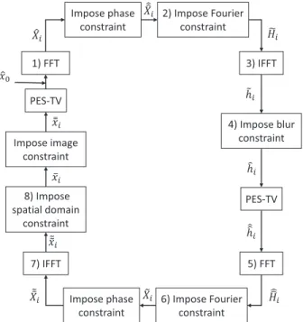
Fig. 10. Sample ﬂuorescent labeled mouse liver tissue images used in experi-ments (a) Im-1, (b) Im-2 (c) Im-3, and (d) Im-4 obtained from [47].

where is a 2D Gaussian filter with and is the high frequency component amplification coefficient. High fre-quency components of is added onto the better focused image . After this step the edge-enhanced image is successively projected onto the phase and ESTV sets in an iterative manner. The image shown in Fig. 6(c) is obtained after 100 iterations.

Obviously, we cannot present PSNR values but the image shown in 6(c) has clearer features compared to 6(a). After 100 iterations we did not observe any improvements in 6(c).

In Fig. 7 another restoration example is shown. In Fig. 8 a third restoration example is shown. Clearly, axial information positively contributed to the deblurring process in Figs. 6, 7 and 8.

In Fig. 9(a) and (b) two differentially focused immunoﬂuo-rescence z-stack images of CD133 positive Huh7 liver cancer cells are shown, respectively. High frequency information from the image is combined with using (21) with and . The image shown in Fig. 9(c) is obtained using suc-cessive phase and ESTV projections after 20 set of iterations. As a result, blurred regions of are clearly visible in Fig. 9.

B. 2D Simulated Blind Deconvolution Using Ayers-Dainty Method

The contribution of phase and ESTV sets to a blind decon-volution problem is also evaluated using different ﬂuorescence (FL) microscopy images obtained at Bilkent University as a part of a project funded by Turkish Scientiﬁc Research Council and German BMBF to track the motility and migration of cells.

(8)

TABLE I

DECONVOLUTIONRESULTS FORFL MICROSCOPICIMAGESBLURRED BY AGAUSSIANFILTERWITHDISCSIZE20AND . PSNR (DB) VALUES AREREPORTED

Fig. 11. Sample deblurring results for “im-7”: (a) Original image, (b) blurred image (Gaussian ); , (c) Image obtained by Ayers-Dainty with Phase and ESTV sets; , (d) Ayers-Dainty method; , (e) image obtained using [16]; . The blurring ﬁlter estimate for each case is shown in the bottom right corner.

The contact inhibition phenomena as a result of cell migration was ﬁrst described in 1950s [46] in cultured cells which in-dicated that cell migration and motility are under the control of cell signaling. Cell migration and motility is a cellular ac-tivity that occurs during various stages of the life cycle of a cell under normal or pathological conditions. Embryonic de-velopment, wound-tissue healing, inﬂammation, angiogenesis,

cancer metastasis are some of the major cellular activities that involve cell motility.

We used a video object tracker to track cells in our research. But the performance was very poor because the FL cell images were very smooth. Therefore we decided to develop a blind convolution method to obtain sharp cell images. After blind de-convolution, cells have clear features and sharper edges which can be used by video object trackers to track the motility of in-dividual cells. In this application we do not have the z-stack im-ages. We only have a slice of the FL image stack. The deconvo-lution operation is performed only the current image slice. The 2D image sequence is obtained using upright fluorescence mi-croscope Nikon Eclipse 50i. We did not use its widefield mode but this microscope can be also used in widefield mode.

In order to evaluate PSNR we selected relatively sharp cell images from FL images and we synthetically blurred them using a 20 20 Gaussian ﬁlter with . We also visually checked the results of our algorithm on naturally blurred images. We tested proposed method against blind Ayers-Dainty [30] to observe the improvement. In Ayers-Dainty based methods, we started by an impulse image in which only one component was nonzero, as the initial guess. This way we ensured that all the frequency components would have a nonzero magnitude value. Furthermore we compared our method with another blind deconvolution method proposed in [16], which achieve deblurring by minimizing a regularization cost. Unfortunately, this method did not produce successful results in FL images.

In Fig. 10, some sample images are shown that are used in experimental studies. Ayers-Dainty method is compared with its own extension using FT phase and ESTV sets.

For Ayers-Dainty based methods, we limited the number of iterations to 300 and stopped the iterations when the estimation difference of consecutive iterations became smaller than a pre-scribed threshold. We have the results of standard Ayers-Dainty method [30], Ayers-Dainty and ESTV set, Ayers-Dainty and phase set, and the proposed Ayers-Dainty with phase and ESTV sets. The comparison of the PSNR performances of these algo-rithms is given in Table I.

We also used blind deconvolution method proposed in [16] to deblur FL microscopy images as shown in Table I. The PSNR

(9)

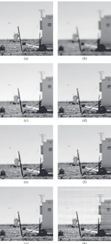
Fig. 12. The deconvolution results for FL image downloaded from [http://bigwww.epﬂ.ch/algorithms/mltldeconvolution/] (a) blurred image, (b) deblurred by the blind deconvolution using phase information (the images and the codes are provided in http://signal.ee.bilkent.edu.tr/BlindDeconvolu-tion.html), (c) deblurred by Ayers and Dainty's algorithm, and (d) Deblurred by Xu et al.'s algorithm [7], which has clear artifacts in blue channels.

performance of this algorithm is not as good as the Ayers-Dainty method. Image deblurring results for “im-7” is shown in Fig. 11. The bold PSNR values are the best results for a given image. We observed that best blind deconvolution results are obtained with Ayers-Dainty method using phase and ESTV set in gen-eral in our FL image test set. The method described in [16] cannot improve ﬁne details of FL images as shown in Fig. 11 and Table I. In the following web-page you may ﬁnd the MATLAB code of projections onto and and example FL images which four of them are shown in Fig. 10. We have the Matlab source codes together with more examples in our web-page: http://signal.ee.bilkent.edu.tr/BlindDeconvolution.html.

In another set of experiments, we used the FL image shown in Fig. 12(a) which is blurred by an unknown ﬁlter or captured with a focus blur [48]. This image is deblurred using the blind decon-volution by phase information and its output is compared with Ayers and Dainty's and Xu et al.'s algorithm [7]. The deblurred image using the blind deconvolution by phase information and , Ayers and Dainty's algorithm, and the Xu et al.'s algo-rithm are shown in Fig. 12(b), 12(c), and 12(d), respectively.

Ayers and Dainty's method sometimes does not converge as shown in Fig. 12(c). Xu et al.'s algorithm also diverges when we select “default” option. It does not diverge when we select “small” kernel option but the result is far from perfect as shown in Fig. 12. The blue channel has clear artifacts. Sets and can be also incorporated into Xu et al.'s method for sym-metric kernels but we do not have an access to the source code. We get the best results when we use and in a succes-sive manner as shown in Fig. 12(b).

VI. CONCLUSION

Both FT phase and the epigraph set of the TV function are closed and convex sets. They can be used as a part of itera-tive microscopic image deblurring algorithms because blurring functions can be assumed to be symmetric in x-y plane. Both sets not only provide additional information about the desired solution but they also stabilize the deconvolution algorithms. It is experimentally observed that phase and ESTV sets signiﬁ-cantly improve the blind deblurring results of Ayers and Dainty's method in FL microscopy images. They can also be used as a part of non-blind deconvolution methods as well.

ACKNOWLEDGMENT

We would like to thank Editors of this Special Issue and the reviewers for their constructive comments.

REFERENCES

[1] P. Campisi and K. Egiazarian, Blind Image Deconvolution: Theory and

Applications. Boca Raton, FL, USA: CRC, 2007.

[2] D. Kundur and D. Hatzinakos, “Blind image deconvolution,” IEEE

Signal Process. Mag., vol. 13, no. 3, pp. 43–64, May 1996.

[3] T. Chan and C.-K. Wong, “Total variation blind deconvolution,” IEEE

Trans. Image Process., vol. 7, no. 3, pp. 370–375, Mar. 1998.

[4] M. Sezan and H. Trussell, “Prototype image constraints for set-theo-retic image restoration,” IEEE Trans. Signal Process., vol. 39, no. 10, pp. 2275–2285, Oct. 1991.

[5] M. Sezan, “An overview of convex projections theory and its applica-tion to image recovery problems,” Ultramicroscopy, vol. 40, no. 1, pp. 55–67, 1992.

[6] H. Trussell and M. Civanlar, “The feasible solution in signal restora-tion,” IEEE Trans. Acoust., Speech, Signal Process., vol. 32, no. 2, pp. 201–212, Apr. 1984.

[7] L. Xu, S. Zheng, and J. Jia, “Unnatural l0 sparse representation for natural image deblurring,” in Proc. IEEE Conf. Comput. Vis. Pattern

Recog. (CVPR), Jun. 2013, pp. 1107–1114.

[8] P. Ye, H. Feng, Q. Li, Z. Xu, and Y. Chen, “Blind deconvolution using an improved l0 sparse representation,” in Proc. 7th Int. Symp. Adv. Opt.

Manuf. Testing Technol. (AOMATT’14), 2014, pp. 928 419–928 419,

Int. Soc. for Opt. and Photon..

[9] J. Boulanger, C. Kervrann, and P. Bouthemy, “Adaptive spatio-tem-poral restoration for 4D ﬂuorescence microscopic imaging,” in Medical

Image Computing and Computer-Assisted Intervention—MICCAI’05,

ser. Lecture Notes in Computer Science, J. Duncan and G. Gerig, Eds. Berlin/Heidelberg, Germany: Springer , 2005, vol. 3749, pp. 893–901.

[10] C. Sorzano, E. Ortiz, M. López, and J. Rodrigo, “Improved Bayesian image denoising based on wavelets with applications to electron mi-croscopy,” Pattern Recog., vol. 39, no. 6, pp. 1205–1213, 2006. [11] S. Acton, “Deconvolutional speckle reducing anisotropic diffusion,”

in Proc. IEEE Int. Conf. Image Process. (ICIP), Sep. 2005, vol. 1, pp. I-5–I-8.

[12] N. Dey, L. Blanc-Féraud, C. Zimmer, P. Roux, Z. Kam, J.-C. Olivo-Marin, and J. Zerubia, “Richardson-Lucy algorithm with total varia-tion regularizavaria-tion for 3D confocal microscope deconvoluvaria-tion,”

(10)

[13] N. Dey, L. Blanc-Féraud, C. Zimmer, P. Roux, Z. Kam, J.-C. Olivo-Marin, and J. Zerubia, “3D microscopy deconvolution using Richardson-Lucy algorithm with total variation regularization,” Res. Rep. RR-5272, 2004.

[14] P. Pankajakshan, B. Zhang, L. Blanc-Féraud, Z. Kam, J.-C. Olivo-Marin, and J. Zerubia, “Blind deconvolution for thin-layered confocal imaging,” Appl. Optimiz., vol. 48, no. 22, pp. 4437–4448, Aug. 2009. [15] B. Zhang, J. Zerubia, and J.-C. Olivo-Marin, “Gaussian

approxima-tions of ﬂuorescence microscope point-spread function models,” Appl.

Optimiz., vol. 46, no. 10, pp. 1819–1829, Apr. 2007.

[16] D. Krishnan, T. Tay, and R. Fergus, “Blind deconvolution using a nor-malized sparsity measure,” in Proc. IEEE Conf. Comput. Vis. Pattern

Recog. (CVPR), 2011, pp. 233–240.

[17] E. Bostan, U. Kamilov, M. Nilchian, and M. Unser, “Sparse stochastic processes and discretization of linear inverse problems,” IEEE Trans.

Image Process., vol. 22, no. 7, pp. 2699–2710, Jul. 2013.

[18] P. L. Combettes and J.-C. Pesquet, “Image restoration subject to a total variation constraint,” IEEE Trans. Image Process., vol. 13, no. 9, pp. 1213–1222, Sep. 2004.

[19] P. L. Combettes and J.-C. Pesquet, “Proximal splitting methods in signal processing,” in Fixed-Point Algorithms for Inverse Problems in

Science and Engineering, ser. Springer Optimization and Its

Applica-tions. New York, NY, USA: Springer, 2011, pp. 185–212. [20] G. Chierchia, N. Pustelnik, J.-C. Pesquet, and B. Pesquet-Popescu,

“Epigraphical projection and proximal tools for solving constrained convex optimization problems,” Signal, Image, Video Process., pp. 1–13, 2014.

[21] A. E. Cetin and M. Toﬁghi, “Projection-based wavelet denoising [lec-ture notes],” IEEE Signal Process. Mag., vol. 32, no. 5, pp. 120–124, Sep. 2015.

[22] M. Toﬁghi, K. Kose, and A. E. Cetin, “Denoising images corrupted by impulsive noise using projections onto the epigraph set of the total variation function (PES-TV,” Signal, Image, Video Process., vol. 9, no. 9, pp. 41–48, 2015.

[23] M. Toﬁghi, K. Kose, and A. E. Cetin, “Denoising using projections onto the epigraph set of convex cost functions,” in Proc. IEEE Int.

Conf. Image Process. (ICIP), Oct. 2014, pp. 2709–2713.

[24] M. Hayes, J. Lim, and A. V. Oppenheim, “Signal reconstruction from phase or magnitude,” IEEE Trans.Acoust., Speech, Signal Process., vol. ASSP-28, no. 6, pp. 672–680, Dec. 1980.

[25] A. V. Oppenheim and J. Lim, “The importance of phase in signals,”

Proc. IEEE, vol. 69, no. 5, pp. 529–541, May 1981.

[26] A. V. Oppenheim, M. H. Hayes, and J. S. Lim, “Iterative procedures for signal reconstruction from Fourier transform phase,” Opt. Eng., vol. 21, no. 1, pp. 211 122–211 122, 1982.

[27] S. Curtis, J. Lim, and A. V. Oppenheim, “Signal reconstruction from one bit of Fourier transform phase,” in Proc. IEEE Int. Conf. Acoust.,

Speech, Signal Process. (ICASSP)., Mar. 1984, vol. 9, pp. 487–490.

[28] L. I. Rudin, S. Osher, and E. Fatemi, “Nonlinear total variation based noise removal algorithms,” Phys. D: Nonlinear Phenom., vol. 60, no. 1–4, pp. 259–268, 1992.

[29] A. Leclaire and L. Moisan, “No-reference image quality assessment and blind deblurring with sharpness metrics exploiting Fourier phase information,” J. Math. Imag. Vis., vol. 52, no. 1, pp. 145–172, 2015. [30] G. R. Ayers and J. C. Dainty, “Iterative blind deconvolution method

and its applications,” Opt. Lett., vol. 13, no. 7, pp. 547–549, Jul. 1988. [31] D. Fish, J. Walker, A. Brinicombe, and E. Pike, “Blind deconvolution by means of the Richardson-Lucy algorithm,” J. Opt. Soc. Amer. A, vol. 12, no. 1, pp. 58–65, 1995.

[32] N. Pustelnik, C. Chaux, and J. Pesquet, “Parallel proximal algorithm for image restoration using hybrid regularization,” IEEE Trans. Image

Process., vol. 20, no. 9, pp. 2450–2462, Sep. 2011.

[33] A. Chambolle, “An algorithm for total variation minimization and ap-plications,” J. Math. Imag. Vis., vol. 20, no. 1–2, pp. 89–97, Jan. 2004. [34] Y. Censor, W. Chen, P. L. Combettes, R. Davidi, and G. Herman, “On the effectiveness of projection methods for convex feasibility problems with linear inequality constraints,” Comput. Optimiz. Applicat., vol. 51, no. 3, pp. 1065–1088, 2012.

[35] M. Toﬁghi, “Image restoration and reconstruction using projections onto epigraph set of convex cost functions,” M.S. thesis, Bilkent Univ., Ankara, Turkey, 2015.

[36] A. E. Cetin, A. Bozkurt, O. Gunay, Y. H. Habiboglu, K. Kose, I. Onaran, R. A. Sevimli, and M. Toﬁghi, “Projections onto convex sets (POCS) based optimization by lifting,” in Proc. IEEE Global Conf.

Signal Inf. Process. (GlobalSIP), 2013, p. 623.

[37] D. Youla and H. Webb, “Image restoration by the method of convex projections: Part 1 theory,” IEEE Trans. Med. Imag., vol. MI-1, no. 2, pp. 81–94, 1982.

[38] A. E. Cetin and A. Tekalp, “Robust reduced update Kalman ﬁltering,”

IEEE Trans. Circuits Syst., vol. 37, no. 1, pp. 155–156, Jan. 1990.

[39] A. E. Çetin and R. Ansari, “Convolution-based framework for signal recovery and applications,” J. Opt. Soci. Amer., vol. 5, no. 8, pp. 1193–1200, Aug. 1988.

[40] H. Trussell and M. R. Civanlar, “The Landweber iteration and projec-tion onto convex set,” IEEE Trans. Acoust., Speech, Signal Process., vol. ASSP-33, no. 6, pp. 1632–1634, 1985.

[41] H. Stark, D. Cahana, and H. Webb, “Restoration of arbitrary ﬁnite-energy optical objects from limited spatial and spectral information,”

J. Opt. Soc. Amer., vol. 71, no. 6, pp. 635–642, Jun. 1981.

[42] P. Combettes, “The foundations of set theoretic estimation,” Proc.

IEEE, vol. 81, no. 2, pp. 182–208, Feb. 1993.

[43] S. Theodoridis, K. Slavakis, and I. Yamada, “Adaptive learning in a world of projections,” IEEE Signal Process. Mag., vol. 28, no. 1, pp. 97–123, Jan. 2011.

[44] I. Yamada, “The hybrid steepest descent method for the variational in-equality problem over the intersection of ﬁxed point sets of nonex-pansive mappings,” in Inherently Parallel Algorithms in Feasibility

and Optimization and their Applications, ser. Studies in Computational

Mathematics. Amsterdam, The Netherlands: Elsevier, 2001, vol. 8, pp. 473–504.

[45] B. Dougherty, 1999, MS Windows NT Iterative Deconvolution [On-line]. Available: http://www.optinav.com/Iterative-Deconvolution.htm [46] M. Abercrombie and J. E. Heaysman, Invasiveness of Sarcoma Cells.

New York, NY, USA: Nature Publishing Group, 1954.

[47] E. Akhan, D. Tuncel, and K. C. Akcali, “Nanoparticle labeling of bone marrow-derived rat mesenchymal stem cells: Their use in differentia-tion and tracking,” BioMed Res. Int., vol. 2015, p. 9, 2015.

[48] C. Vonesch and M. Unser, “A fast multilevel algorithm for wavelet-regularized image restoration,” IEEE Trans. Image Process., vol. 18, no. 3, pp. 509–523, Mar. 2009.

Mohammad Toﬁghi received his B.Sc. in electrical

engineering from Urmia University, Urmia, Iran, in 2012. In 2010, he collaborated with the Advanced Communication Research Institute, Department of Electrical Engineering, Sharif University of Technology, Tehran, Iran. He received his M.Sc. in electrical engineering from the Electrical and Elec-tronics Engineering Department, Bilkent University, Ankara, Turkey, in 2015. He is currently pursuing his PhD in Department of Electrical Engineering, Pennsylvania State University, University Park, PA. His research interests include signal and image processing, computer vision and machine learning.

Onur Yorulmaz received his B.Sc. and M.Sc. degree

in the Electrical and Electronics Engineering Depart-ment, Bilkent University, Ankara, Turkey, in 2012. He is currently working on his PhD studies in the Electrical and Electronics Engineering Department of Bilkent University. His research interests include signal and image processing, computer vision, and machine learning.

Kivanç Köse got his Ph.D. degree from the Electrical

and Electronics Engineering Department, Bilkent University in 2011. He is currently working as a Postdoctoral Research Fellow at Dermatology De-partment, Memorial Sloan-Kettering Cancer Center. He is an associate editor of Signal, Image and Video

Processing journal. He research interests include

signal and image processing, inverse problems in image processing, computer vision and machine learning in medical image processing applications.

(11)

Deniz Cansen Yıldırım received her B.Sc. in

molec-ular biology and genetics from Bilkent University Ankara, Turkey, in 2011. She is currently carrying out her Ph.D. studies at the same department in Bilkent University. Her research interests include discovery of novel small molecule kinase inhibitors against liver cancer and cancer stem cells.

Rengül Çetin-Atalay received her Ph.D. degree in

1997 from Université de Paris-Sud, Orsay, France. She was a French Government scholar during her PhD. She carried out her doctoral studies as a Research Assistant at Ecole Polytechnique, Paris, France. Between 1997–2014, Dr. Cetin-Atalay was a faculty member at Bilkent University. She worked as an Assistant Professor at the Virginia Bioinformatics Institute, Virginia Polytechnic Institute and State University, Virginia, USA, during her sabbatical leave in 2004. She is currently a faculty member at

Middle East Technical University, Ankara, Turkey. Dr. Cetin-Atalay's research interests lie in the ﬁelds of bioinformatics and molecular cellular biology of liver cancer.

A. Enis Çetin got his Ph.D. degree from the

Univer-sity of Pennsylvania in 1987. Between 1987–1989, he was Assistant Professor of Electrical Engineering at the University of Toronto. He has been with Bilkent University, Ankara, Turkey, since 1989. He will be on sabbatical leave at University of California, San Diego, starting Dec. 2015. He was an Associate Editor of the IEEE TRANSACTIONS ON

IMAGEPROCESSINGbetween 1999–2003. Currently,

he is the editor in-chief of Signal, Image and Video

Processing journal and on the editorial boards of

journals Signal Processing and Journal of Advances in Signal Processing

(EURASIP), and Journal of Machine Vision and Applications (IAPR), Springer.

He is currently an Associate Editor of the IEEE Signal Processing Magazine and IEEE TRANSACTIONS ONCIRCUITS, SYSTEMS,ANDVIDEOTECHNOLOGY.

He is a fellow of IEEE. His research interests include signal and image processing, human–computer interaction using vision and speech, audio-visual multimedia databases.