Original Research
Measuring Local RF Heating in MRI: Simulating
Perfusion in a Perfusionless Phantom
Imran B. Akca, BS,
1Onur Ferhanoglu, MS,
1Christopher J. Yeung, PhD,
2Sevin Guney, MSc,
3T. Onur Tasci, MS,
1and Ergin Atalar, PhD
1,4*
Purpose: To overcome conflicting methods of local RF heat-ing measurements by proposheat-ing a simple technique for predicting in vivo temperature rise by using a gel phantom experiment.
Materials and Methods: In vivo temperature measurements are difficult to conduct reproducibly; fluid phantoms intro-duce convection, and gel phantom lacks perfusion. In the proposed method the local temperature rise is measured in a gel phantom at a timepoint that the phantom temperature would be equal to the perfused body steady-state temperature value. The idea comes from the fact that the steady-state temperature rise in a perfused body is smaller than the steady-state temperature increase in a perfusionless tom. Therefore, when measuring the temperature on a phan-tom there will be the timepoint that corresponds to the per-fusion time constant of the body part.
Results: The proposed method was tested with several phantom and in vivo experiments. Instead, an overall aver-age of 30.8% error can be given as the amount of underes-timation with the proposed method. This error is within the variability of in vivo experiments (45%).
Conclusion: With the aid of this reliable temperature rise prediction the amount of power delivered by the scanner can be controlled, enabling safe MRI examinations of pa-tients with implants.
Key Words: RF heating; MRI safety; interventional MRI; metallic implants; perfusion; bioheat equation
J. Magn. Reson. Imaging 2007;26:1228 –1235. © 2007 Wiley-Liss, Inc.
THE RISK OF HAZARDOUS RF heating when doing MRI scans with metallic objects present in the body is well reported. The potential for RF heating is particularly great for long linear conductive objects, such as guide-wires and minimally invasive imaging antennas (1–3).
Most published studies of RF heating with such de-vices have measured temperature changes in fluid or gel phantoms (4 –10). However, the temperature in-creases measured in such phantom studies do not ac-curately reflect the temperature increases that can oc-cur in living patients, primarily because the physiologic effects of bioheat transfer have not been taken into account (11).
The sources of error are several. First, as Smith et al (12) demonstrated, the choice of phantom material has a significant effect on the measured temperature changes in such phantom experiments. Studies that have used fluid phantoms (water or saline) (4 –7) intro-duced the possibility of convective heat transfer (a physiologic phenomenon in most tissues), which non-linearly limits the potential temperature increase, resulting in significant underestimation of the temper-ature change. Studies with gel phantoms (8 –10) re-moved the possibility of convection but can still signif-icantly overestimate (100% or more) or underestimate (50% or more) the temperature change if the gel’s ther-mal conductivity differs from that of the body (12).
Second, no phantom study has attempted to model a crucial heat transfer component—perfusion. All living tissues in the body are perfused, although some, like the eye and cortical bone, have very low perfusion. A worst-case heating scenario has very low perfusion, not zero perfusion (13). Perfusion is a significant compo-nent of bioheat transfer that, if ignored, will result in overestimation of the temperature change. This overes-timation is exacerbated for larger phantoms.
One approach to overcome these limitations has been to measure specific absorption rate (SAR) in phantom studies (14,15) rather than temperature change. Mea-surements of SAR, which is proportional to the initial
rate of temperature increase, are much less susceptible
1
Electrical and Electronic Engineering Department, Bilkent University, Ankara, Turkey.
2
Division of Intramural Research, National Heart, Lung & Blood Insti-tute, National Institutes of Health, Bethesda, Maryland.
3
Institute of Health Sciences, Department of Physiology, Gazi Univer-sity, Ankara, Turkey.
4
Department of Radiology, Johns Hopkins University School of Medi-cine, Baltimore, Maryland.
I.B. Akca is now with Institute of Material Science and Nanotechnology, Physics Department, Bilkent University, Ankara, Turkey.
O. Ferhanoglu is now with the Department of Electrical and Electronics Engineering, Koc University, Istanbul, Turkey.
T.O. Tasci is now with the Department of Bioengineering, University of Utah, Salt Lake City, Utah.
Contract grant sponsor: National Institutes of Health; Contract grant number: R01 RR 15396; Contract grant sponsor: European Commis-sion; Contract grant number: FP6 Marie Curie International Reintegra-tion Grant.
*Address reprint requests to: Ergin Atalar, PhD, Bilkent University, Department of Electrical and Electronics Engineering, Bilkent 06800, Ankara, Turkey. E-mail: [email protected]
Received March 17, 2007; Accepted August 3, 2007. DOI 10.1002/jmri.21161
Published online in Wiley InterScience (www.interscience.wiley.com).
to the heat transfer conditions. Therefore, phantom measurements are more likely to properly simulate physiological conditions. However, it is temperature, and not SAR, that ultimately causes tissue damage. Thus, the conclusions of these studies are also limited. The goal of this study is to demonstrate a method for accurately predicting in vivo temperature changes near metallic implants during MRI, rather than simply mea-suring the raw temperature changes that can be gen-erated in a nonphysiologic phantom material. This method is able to simulate the effects of physiologic thermal conductivity and perfusion in a phantom that has no actual perfusion (nor necessarily even the cor-rect thermal conductivity), thus providing an unambig-uous measure of a metallic device’s RF safety.
MATERIALS AND METHODS
Figure 1 summarizes the limitations of phantom stud-ies. Top row of Figure 1 shows the transfer of RF power,
P, from the RF transmitter (usually body coil), into an
SAR distribution in the patient and ultimately to a tem-perature increase, ⌬T, during a normal clinical MRI scan on a living patient. The SAR distribution depends primarily on the geometric positioning of the patient relative to the transmitter and the tissue’s electrical properties: electrical conductivity, and electrical per-mittivity,⑀. The SAR distribution is converted to a tem-perature distribution, depending primarily on the tis-sue’s thermal properties: thermal diffusivity, ␣, and perfusion time constant, (time constant of tempera-ture rise when the tissue is exposed to uniform heat-ing). Bottom row of Figure 1 shows how a phantom experiment typically fails to account for all the factors that affect the measured temperature increase. Usually the electrical properties of the tissues are adequately modeled by a tissue-equivalent lossy dielectric. How-ever, the thermal properties of the phantom are ne-glected: the thermal conductivity is typically unknown, and there is no perfusion.
Predicting Perfused Body Temperature Rise Using Perfusionless Phantom Temperature Data
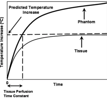
The new method proposed here is summarized in Fig. 2. In this method the local temperature rise is measured in a gel phantom at a timepoint that the phantom tem-perature would be equal to the perfused body steady-state temperature value. The idea comes from the fact that the steady-state temperature rise in a perfused body is smaller than the steady-state temperature in-crease in a perfusionless phantom. The timepoint that the phantom temperature equals to the perfused body steady-state temperature value may depend on the heat distribution. Here we will first calculate this timepoint for a uniform heating case and then investigate the errors resulting from using the same timepoint for pre-dicting the perfused body steady-state temperature rise.
The bioheat transfer equation (16) describes how an SAR distribution is converted to a distribution of tem-perature change,⌬T, in the presence of conduction and perfusion heat transfer:
d⌬T共rជ,t兲 dt ⫽ ␣ⵜ 2⌬T共rជ,t兲 ⫺1 ⌬T共rជ,t兲 ⫹ 1 cSAR共rជ兲 (1)
where r and t are the space and time coordinates, re-spectively,␣ is the thermal diffusivity, ⵜ2is the Lapla-cian operator, c is the heat capacity, is the perfusion time constant ( ⫽ c/cb/bm, wherebis the mass
den-sity of the perfusing blood, cbis the heat capacity of the
blood, and m is the volumetric flow rate of blood per unit mass of tissue). This equation models the physio-logic system labeled “Bioheat Transfer” in Fig. 1, top row.
When the heating is uniform, the Laplacian term of Eq. (1)] is zero. The steady-state temperature becomes
Figure 2. Pictorial representation of the proposed theorem: On the phantom graph, the temperature increase at tissue perfusion time constant is equal to temperature increase of in vivo case at the steady state.
Figure 1. Top row: Generalized schematic of RF heating of patients in an MRI scanner. Power, P, from the RF transmitter is deposited in the tissue as a specific absorption rate distri-bution (SAR). This is in turn transformed into a local temper-ature increase,⌬T, depending on the electrical conductivity, , and the electrical permittivity, ⑀, the thermal diffusivity, ␣, perfusion time constant,, and heat capacity, c. Bottom row: Schematic diagram of RF heating of gel phantoms in an MRI scanner. Electrical conductivity, electrical permittivity, ther-mal diffusivity, and heat capacity may not exactly match phys-iologic values. Perfusion is typically absent.
/cSAR. On the other hand, uniform heating of a per-fusionless phantom has no steady-state value and the temperature rise is t/cSAR. Therefore, the temperature of the perfusionless phantom becomes equal to the steady-state temperature of the perfused body when time is equal to the perfusion time constant,.
When the heating is not uniform, the analysis is rather involved. It was previously shown that for the special case of localized RF heating in deep tissues, the type that occurs with invasive or implanted metal ob-jects, this equation can be reduced to a linear, shift-invariant system. As such, it is fully characterized by its impulse response function, also called Green’s function (2). The bioheat equation can be solved, then, by simply convolving the SAR distribution by this Green’s func-tion to yield the resulting temperature distribufunc-tion, shown here for steady-state conditions (2):
⌬Tss共rជ0兲 ⫽
冕
SAR共rជ兲G共rជ ⫺ rជ0兲dV (2)where the integral is performed over the whole volume,
V, and G is the Green’s function given in spherical
coordinates as (2):
G共r兲 ⫽ 1
4␣tctr
e⫺vr (3)
where ⫽ 1/
冑
␣, is a lumped perfusion constant. In this equation tissue-specific parameters are denoted by subscript t. The Green’s function represents the tem-perature distribution in the body resulting from a point SAR source. The temperature increase at any position,r
ជ0, is a weighted average of the local SAR distribution. For example, in the case of a spherically symmetric SAR distribution centered at the origin, this integral be-comes:
⌬Tss共0兲 ⫽
冕
0 ⬁
SAR共r兲G共r兲4r2dr (4)
where r is the radius, 4r2is the Jacobian.
Spatial 3D Fourier transform of the Green’s function yields the following:
G共兲 ⫽ ct 1 1⫹ 2 2 (5)
where, is the spatial radial frequency variable of the Fourier transform. We will compare this value with the phantom measurement value.
In a perfusionless phantom with identical thermal conductivity and diffusion as in the in vivo case, the Green’s function takes the following time-dependent form (2): G(r,t)⫽ 1 cp共4␣pt兲3/2 exp
冉
⫺ r 2 4␣pt冊
(6)which represents temperature distribution in a phan-tom as a function of time when an impulse SAR is applied to a point at the center of the phantom. In this equation, phantom-related parameters are denoted by subscript p.
When a unit step heating is applied to a point at the center of a phantom for a period of time,, which is the perfusion time constant of the tissue of interest, the phantom temperature distribution can be found as:
Gp共r兲 ⫽
冕
0
x
G共r,t兲dt (7)
In order to compare this perfusionless phantom tem-perature distribution with in vivo temtem-perature distribu-tion, we take its 3D spatial Fourier transform:
Gp共兲 ⫽ cp 1⫺ exp共 ⫺ 2/ p 2兲 2/ p 2 (8) where p⫽ 1/
冑
␣pAs can be seen, Eqs. (5) and (8) are different. A careful analysis of these equations, however, yields striking similarities. If one assumes that the thermal diffusion constants and the heat capacity of the gel phantom are designed to be equal to that of tissue (ct⫽ cp,␣ ⫽ ␣p), the
coefficients of these equations become equal. In addi-tion, this assumption makes lumped perfusion con-stants equal ( ⫽ p). Both functions given in Eqs. (5)
and (8) depend only on the radial component of the frequency normalized with the lumped perfusion con-stant,. The functions 共1 ⫺ exp共 ⫺ 2兲兲/2 and 1/共1 ⫹ 2兲 are very similar functions (Fig. 3a), showing a maximum deviation of 30% when the radial spatial fre-quency is 1.34 (Fig. 3b). This means that when a gel phantom temperature measurement is conducted at the time of perfusion time constant, the maximum pos-sible overestimation is 30%.
For both Green’s functions (phantom and in vivo cases), ctand cp are simple scaling functions. In cases
where the heat capacity of the phantom and tissue do not match, the mismatch can be corrected by simple scaling of the phantom temperature using cp/ct ratio.
Typical values of this ratio are in the range of 1 to 3 (Table 1).
Here is the proposed algorithm:
1. Make a gel phantom that matches as closely as possible the geometric, electrical properties and the thermal conductivity of the situation in which the metallic device will be used. The electromag-netic part of the problem, particularly geometry, electrical permittivity, and electrical conductivity, must be properly simulated physically. Fortu-nately, this is what many studies have already attempted to do. One may want to orient the device relative to the RF transmitter in a way that will generate the worst-case coupling, not necessarily
worst-case absolute heating (adjustments such as moving the phantom off-center or changing the depth of the device in the phantom can be ac-counted for in Step 5).
2. Appropriately position the selected temperature probe at the suspected hotspots and record the temperature rise at the hotspots as a function of applied SAR.
3. Report the temperature rise after the power has been applied for seconds, where is the perfusion time constant of the tissue in which the metallic device will be placed. This temperature is the ex-pected in vivo temperature rise. Values for perfu-sion time constants can be from Table 1 or derived from literature tables (17–22).
4. Optional: Correct the estimated temperature in-crease with the ratio of the heat capacity of the phantom and tissue. Values of heat capacity can be obtained from the literature or from Table 1. This scaling step is not necessary if the estimated temperature is normalized with measured SAR at one other point on the phantom (as in Step 5.) Otherwise, scaling is necessary.
5. If measuring the safety of a passive device that is completely inside the body, measure the applied SAR in the region of hotspots with the exact same configuration except with the metallic device re-moved, and normalize the predicted in vivo tem-perature rise with the applied SAR yielding the safety index (23). Without this normalization step the value reported in Step 3 will only be applicable to the specific geometry configured in Step 2. Cer-tain geometric effects such as moving the phan-tom off-center or changing the depth of the object in the phantom will change the absolute amount of heating measured near the device, but this will be caused by a proportional change in the heating at the same location without the device in place. These effects can be accounted for with this nor-malization step. The normalized temperature rise, namely the safety index (23), has previously been shown to be a measure of the possible in vivo temperature change that can occur with a metallic device, which is independent of geometry.
We have tested the algorithm with in vivo experi-ments. With a copper wire of length 110 cm as the ablation probe, we compared predictions of in vivo tem-perature change in agarose gel phantom experiments with the actual temperature rise measured in various tissues in live rabbits.
Experimental Design Considerations
The experimental set-up is shown in Fig. 4. A 110-cm, 1-mm diameter copper wire was inserted 1.5 cm into the tissue/phantom to induce current that causes tem-perature increase near the tip of the wire. The position and orientation of both the wire and the rabbit within the scanner bore affect the coupling of the wire to the
Figure 3. a: Comparison of Fourier transform of in vivo Green’s function with phantom Green’s function. Both X and Y axes are normalized for ease of comparison. b: Percent error in the phantom measurement as a function of normalized fre-quency. Maximum deviation when the radial spatial frequency is 1.34 should be noted.
Table 1
Thermal Properties of Different Tissues of Rabbit Tissue Type (rabbit) Perfusion (mL/100g/min) Time Constant (sec)
Tissue Heat Capacity (ct) (J/kgK) Thermal Diffusivity (␣) (cm–2/sec) References Fat 9–13 275–396 2500 0.1 27, 32 Brain 35–75 72–150 3700 0.143 27, 31 Liver 65–234 22–85 3600 0.136 27, 28, 29 Kidney 200–500 12–30 3900 0.128 27, 29, 30
RF transmitter, and hence the amount of heat at the wire tip. This geometric variability was kept as con-trolled as possible by carefully positioning the wire in the same position and orientation in the scanner and at the same depth in the rabbit for each experiment. A fiberoptic probe (FISO Technologies, Ste. Foy, Canada) was attached next to the wire for temperature measure-ment. The position of the wire and the fiberoptic probe with respect to each other was very crucial in our case, since the sensitive region of the fiberoptic probe was 1 cm behind the tip.
Phantom Experiment
Ideally, one should make an agarose gel phantom that matches the geometric, electrical, and thermal proper-ties (except perfusion) of the tissue in which the metallic device will be used. In our case, to test the theory, we used a cylindrical homogeneous agarose gel phantom (Agarose A5093, Sigma-Aldrich, Steinheim, Germany) which is a high water content (99%) material thus suit-able for simulating tissue. The length of the cylindrical phantom was 10 cm and the diameter was 15 cm. Both the phantom and the rabbits weighed⬇2 kg. The rela-tive electrical permittivity (70) and conductivity (0.56 S/m) of the gel were deduced from measurements at 64 MHz with a Network Analyzer (HP5763, Agilent Tech-nologies, Santa Clara, CA). The specific heat capacity of the phantom was 3880 J/kgK. The values indicate that the phantom best mimics kidney tissue; however, com-pensation is possible as mentioned previously for other tissues, especially fat, which exhibits different proper-ties than most other tissues.
The experiment lasted for nearly 2000 seconds and the temperature versus time graph of the phantom was used as a reference for the comparison between exact and the predicted steady state temperature values of different tissues.
Rabbit In Vivo Experiment
The experimental prediction of in vivo temperature change was validated with rabbit experiments (n⫽ 8). Animal preparation was performed as follows. First, the rabbit was anesthetized with a mixture of 35 mg/kg ketamine and 5 mg/kg xylazine through intramuscular infusion. Ketamine was repeated each hour.
Experiments were performed on a GE Signa (Wauke-sha, WI) 1.5T scanner using an steady-state free pre-cession (SSFP) pulse sequence. The transmit gain was fixed to 15–18 dB, overriding any prescan values. Fiber optic temperature data from four tissues (fat, kidney, liver, and brain) were collected and compared with the data taken from the phantom experiment.
RESULTS
At the end of the phantom experiment a temperature– time curve was obtained for different input powers. All the curves were normalized with respect to the power applied in the phantom experiment. This normalized temperature–time curve was the reference point of our preceding calculations. Predicted temperature rise cor-responding to the four different tissue types (fat, brain, liver, kidney) were calculated from thermal parameters obtained from the literature (Fig. 5).
Two sets of experiments were conducted. In the first set, one phantom and one animal experiment were done. In the second set, one phantom experiment and seven animal experiments were conducted. The data for the second set of experiments are shown in Fig. 6. The regions shown with dashed lines refer to estimated ranges based on phantom experiments for each tissue. The results of all experiments are summarized in Table 2. The average of temperature increase in in vivo and phantom data of all experiments are calculated for each tissue type separately. The difference between the predicted temperature rise and this averaged value are reported as errors. Given the high variability of in vivo experiments, it is not possible to deduct a definite
con-Figure 5. The result of the phantom experiment. The perfu-sion time constants of four tissues (fat, liver, kidney, and brain) and corresponding temperature increases are shown. Figure 4. Experimental setup of the in vivo and phantom
clusion on the errors as a function of the tissue type. Instead, an overall average of 30.8% error can be given as the amount of underestimation with proposed method. This error is within the variability of in vivo experiments (45%).
DISCUSSION
In reality, the device under investigation may be placed in several tissues. In such occasions the perfusion time constant of the tissue that contains the hotspot is to be taken into account, since the greatest temperature in-crease is determined by this local area. Thus, the pre-diction method described here is not limited to homo-geneous tissue.
In the experiment the criterion for choosing the length of the wire was to ensure high signal-to-noise ratio (SNR) temperature data (⬎2°C temperature in-crease) to be observed. This could also be achieved using different wire length, inserted length, wire radial position, phantom radial position, and transmit gain parameter. The sequence is also not a determining pa-rameter for the experiment; the prediction is valid once conditions in the phantom experiment mimic the in vivo conditions.
While describing the mathematical background on the proposed temperature rise prediction method, it was shown that even if all the thermal and electrical properties of the gel phantom and the tissue match,
Figure 6. Temperature increase versus time graphs for four tissues of rabbit. The regions shown by dashed lines are estimated ranges based on the phantom experiment. Phantom data scaled by heat capacity and applied power of corresponding tissues.
Table 2
Comparison of Average Values of Predicted and Measured Temperature Increases for Different Tissues Tissue
Type
Average Value of In Vivo Temperature
Increase (°C)
Average Value of Scaled Estimated Temperature Increase (°C) (calculated from phantom data at t⫽ )
Average Error in Estimate (%) Fat 5.7 6.0 5.0 Kidney 6.3 2.7 ⫺57.0 Liver 4.6 3.7 ⫺19.0 Brain 9.2 4.4 ⫺52.0
there may be up to 30% overestimation in the predicted temperature rise based on the distribution of the SAR. Given the variability in the tissue thermal and electrical properties, this error is relatively insignificant. Here we will concentrate on the other error sources.
After doing several phantom and in vivo experiments, an average 30.8% underestimation with our tempera-ture prediction method was observed. As can be seen from Table 2, the temperature increase is overestimated in fat and for liver, kidney, and brain it is underesti-mated. Two of four experiments have errors within 30%. There may be several reasons for this error.
One reason for the error is the mismatch between thermal and electrical properties of the phantom and the tissues. More accurate results may be obtained if different gels were used for simulating each tissue. Electrical properties of the gel phantom and all the tissues (except fat) are similar (http://www.fcc.gov/fcc-bin/dielec.sh), but we did not attempt to match the thermal conductivity of the phantom to the tissues. Both the phantom and tissues involved in these exper-iments (except fat) are water-dominant; therefore, spe-cific heat capacity values are expected to be similar.
To overcome the temperature fluctuations in animal experiments, it is suggested to use isolated perfused bovine tongue rather than in vivo (24). Although iso-lated perfused bovine tongue models the perfusion, it is not a perfect model. It lacks body thermal regulation. Electrical and thermal properties of tongue are different than other parts of the body. In addition, this method will introduce extra error sources such as nonunifor-mity of perfusion. In our studies we used an in vivo animal model that has also its own problems, but ob-taining more realistic results is possible using this method.
Another possible source of error is the mismatch be-tween the perfusion values gathered from the literature and the actual in vivo experiment. To minimize the error a wide range of perfusion values from several sources were gathered, as seen in Table 1.
In local heating, thermal diffusivity also plays a sig-nificant role. The diffusivity of phantom was measured as 0.15 mm2/s; this value is higher than the diffusivity of tissue as seen in Table 1. This results in underesti-mation of the temperature with phantom experiments. Last, but not least, placement errors of the tempera-ture probe during experiments introduce significant er-rors. The temperature rise is local. If the position of the temperature probe varies even less than a millimeter between in vivo and phantom experiments, there will be significant mismatch between results. In order to min-imize this error, we paid maximum attention to this problem. However, neither agarose nor body is trans-parent and, therefore, it was not possible to observe if there was a change in the position of the probe. We believe that this is a significant source of the experi-mental errors and may explain the high variability of our in vivo experiments. Calculated average bias may have some contribution to this problem.
Although there are some experimental errors and bias, we believe that the proposed in vivo temperature prediction method is a useful method for measuring the
safety of interventional devices or metallic implants in-side the body during an MRI examination.
In conclusion, conflicting methods on the evaluation of RF heating in the MR literature led us to construct a practical method for measuring local RF heating. In this study we have presented a method of predicting in vivo temperature increase by using a straightforward aga-rose gel phantom experiment. We propose that the steady-state tissue temperature is the phantom tem-perature change for a period of the tissue perfusion time constant. The proposed method was explained by a theory and was tested with several phantom and in vivo experiments. We believe that by reliable test tech-niques such as the one described here the amount of possible temperature rise in the body with an implant during an MRI exam will be predicted accurately. With the aid of this reliable prediction the amount of power delivered by the scanner will be controlled, enabling safe MRI examinations of patients with implants.
REFERENCES
1. Nitz WG, Oppelt A, Renz W, Manke C, Lenhart M, Link J. On the heating of linear conductive structures as guidewires and catheters in interventional MRI. J Magn Reson Imaging 2001;13:105–114. 2. Yeung CJ, Atalar E. A Green’s function approach to local RF heating
in interventional MRI. Med Phys 2001;28:826 – 832.
3. Shellock FG. Radiofrequency energy-induced heating during MR procedures: a review. J Magn Reson Imaging 2000;12:30 –36. 4. Sommer T, Vahlhaus C, Lauck G, et al. MR imaging and cardiac
pacemakers: in vitro evaluation and in vivo studies in 51 patients at 0.5 T. Radiology 2000;215:869 – 879.
5. Tronnier VM, Staubert A, Ha¨hnel S, Sarem-Aslani A. Magnetic resonance imaging with implanted neurostimulators: An in vitro and in vivo study. Neurosurgery 1999;44:118 –125.
6. Ladd ME, Quick HH. Reduction of resonant RF heating in intravas-cular catheters using coaxial chokes. Magn Reson Med 2000;43: 615– 619.
7. Achenbach S, Moshage W, Diem B, Bieberle T, Schibgilla V, Bach-mann K. Effects of magnetic resonance imaging on cardiac pace-makers and electrodes. Am Heart J 1997;134:467– 473.
8. Smith CD, Kildishev AV, Nyenhuis JA, Foster KS, Bourland JD. Interactions of magnetic resonance imaging radio frequency mag-netic fields with elongated medical implants. J Appl Phys 2000;87: 6188 – 6190.
9. Nyenhuis JA, Kildishev AV, Bourland JD, Foster KS, Graber G, Athey TW. Heating near implanted medical devices by the MRI RF-magnetic field. IEEE Trans Magn 1999;35:4133– 4135. 10. Shellock FG. Metallic neurosurgical implants: evaluation of
mag-netic field interactions, heating, and artifacts at 1.5-Tesla. J Magn Reson Imaging 2001;14:295–299.
11. Yeung CJ, Atalar E. Estimating in vivo temperature changes due to localized RF heating from interventional devices. In: Proc 9th ISMRM, Glasgow, Scotland; 2001:1756.
12. Smith CD, Nyenhuis JA, Foster KS. A comparison of phantom materials used in evaluation of radiofrequency heating of im-planted medical devices during MRI. In: Proc 23rd Annual Interna-tional Conference IEEE Eng Med Biol Soc, Istanbul; 2001. 13. Busch HJM, Vollmann W, Schnorr J, Gro¨nemeyer HWD. Finite
volume analysis of temperature effects induced by active MRI im-plants with cylindrical symmetry. BioMed Eng OnLine 2005;4:25– 42.
14. Yeung CJ, Atalar E. RF transmit power limit for the barewire loop-less catheter antenna. J Magn Reson Imaging 2000;12:86 –91. 15. Luechinger R, Weber OM, Bieler M, Boesiger P. Heat distribution
near pacemaker lead tips. In: Proc 9th Annual Meeting ISMRM, Glasgow, Scotland; 2001:1759.
16. Pennes HH. Analysis of tissue and arterial temperatures in the resting human forearm. J Appl Physiol 1948;1:93–122.
17. Nevels RD, Arndt GD, Raffoul GW, Carl JR, Pacifico A. Microwave catheter design. IEEE Trans Biomed Eng 1998;45:885– 890.
18. Cooper TE, Trezek GJ. Correlation of thermal properties of some human tissue with water content. Aerospace Med 1971;42:24 –27. 19. Valvano JW, Cochran JR, Diller KR. Thermal conductivity and diffusivity of biomaterials measured with self-heated thermistors. Int J Thermophys 1985;6:301–311.
20. Guy AW, Lehmann JF, Stonebridge JB. Therapeutic applications of electromagnetic power. In: Proc IEEE 1974;62:55–75.
21. Tropea BI, Lee RC. Thermal injury kinetics in electrical trauma. J Biomech Eng 1992;114:241–250.
22. Shitzer A, Eberhart RC. Heat transfer in medicine and biology. New York: Plenum; 1985. p 141.
23. Yeung CJ, Susil RC, Atalar E. RF safety of wires in interventional MRI: Using a safety index. Magn Reson Med 2002;47:187–193. 24. Raaymakers BW, Crezee J, Lagendijk JJW. Modelling individual
temperature profiles from an isolated perfused bovine tongue. Phys Med Biol 2000;45:765–780.
25. Ocali O, Atalar E. Intravascular magnetic resonance imaging using a loopless catheter antenna. Magn Reson Med 1997;37:112–118. 26. Polk C, Postow E. Handbook of biological effects of electromagnetic
fields, 2nd ed. New York: CRC Press; 1996. p 92–93.
27. U.S. Department of Health and Human Services, Food and Drug Administration, Center for Devices and Radiological Health. Guid-ance for the submission of premarket notifications for magnetic resonance diagnostic devices. Rockville, MD: US DHHS FDA; 1998.
28. International Electrotechnical Commission. Medical electrical equipment. Part 2. Particular requirements for the safety of mag-netic resonance equipment for medical diagnosis. International Standard 60601-2-33. Geneva: IEC; 1995.
29. Hirate A, Watanabe S, Kojima M, et al. Computational verification of anesthesia effect on temperature variations in rabbit eyes ex-posed to 2.45 GHz microwave energy. Bioelectromagnetics 2006; 27:602– 612.
30. Materne R, Beers BE, Smith AM, et al. Non-invasive quantification of liver perfusion with dynamic computed tomography and a dual-input one-compartmental model. Clin Sci 2000;99:517–525. 31. Jones SC, Parker DS. Mammary blood flow and cardiac output in
the conscious lactating rabbit. J Comp Physiol 1980;138:31–34. 32. Anetzberger H, Thein E, Becker M, Walli AK, Messmer. Validity of
fluorescent microspheres method for bone blood flow measurement during intentional arterial hypotension. J Appl Physiol 2003;95: 1153–1158.
33. Eyret JA, Essex TJH, Flecknells PA, Bartholomew PH, Sinclair JI. A comparison of measurements of cerebral blood flow in the rabbit using laser Doppler spectroscopy and radionuclide labelled micro-spheres. Clin Phys Physiol Meas 1988;9:65–74.
34. Carroll JF, Huang M, Hester RL, Cockrell K, Mizelle L. Hemody-namic alterations in hypertensive obese rabbits. Hypertension 1995;26:465– 470.