VIBRATION ANALYSIS OF ROTATING TIMOSHENKO BEAMS WITH DIFFERENT MATERIAL DISTRIBUTION PROPERTIES
1Özge ÖZDEMİR
1Istanbul Technical University, Faculty of Aeronautics and Astronautics, Aeronautical Engineering Department,
İSTANBUL
(Geliş/Received: 29.07.2018; Kabul/Accepted in Revised Form: 02.11.2018)
ABSTRACT: In this study, vibration characteristics of functionally graded rotating Timoshenko beams that undergoes flapwise bending vibration are analysed. Beam models with different material distribution properties are considered. The energy expressions are derived by introducing several explanotary figures and tables. Applying the Hamilton’s Principle to the derived energy expressions, governing differential equations of motion and the boundary conditions are obtained. Related formulation is coded by using MATLAB and in the solution part, the equations of motion, including the parameters for the rotary inertia, shear deformation, power law index parameter and slenderness ratio are solved using an efficient mathematical technique, called the differential transform method (DTM). Natural frequencies of the modeled beams are obtained. Increasing effects of the slenderness ratio and the rotational speed and the decreasing effect of the power-law index on the natural frequencies are investigated. Moreover, differences between the natural frequencies of the beam models with different material distribution characteristics is noticed and examined. Obtained results are distributed in several tables.
Keywords: Differential Transform Method, Functionally Graded Beam, Rotating Timoshenko Beam Fonksiyonel Derecelendirilmiş Dönen Timoshenko Kirişlerin Titreşim Analizi
ÖZ: Bu çalışma kapsamında, düzlem dışı eğilme (flaplama hareketi) deplasmanı altında fonksiyonel derecelendirilmiş, dönen Timoshenko kirişlerin titreşim analizi yapılmıştır. Farklı malzeme dağılımlarına sahip kiriş modelleri incelenmiş ve enerji ifadeleri, çeşitli şekil ve tablolar kullanılarak çıkarılmış ve bu enerji denklemlerine Hamilton Prensibi uygulanarak hareket denklemleri ve sınır şartları elde edilmiştir ve ilgili denklemler, MATLAB programında kodlanmıştır. Çözüm aşamasında; dönme ataleti, kayma etkisi, malzeme dağılımı üstel fonksiyonu, kiriş narinlik oranı gibi çok çeşitli parametrelerin katıldığı hareket denklemleri ve sınır şartlarına, etkin ve hızlı bir matematiksel yöntem olan Diferansiyel Dönüşüm Yöntemi (Differential Transform Method) uygulanmıştır. Modellenen kirişlere ait doğal frekanslar hesaplanmıştır. Narinlik oranı ve dönme hızının frekanslar üzerindeki yükseltici etkileri ve malzeme dağılımı ile ilgili olarak güç indeksinin, frekanslar üzerindeki azaltıcı etkisi incelenmiştir. Ayrıca, farklı malzeme dağılım karakterlerine sahip kirişlere air frekans değerleri arasındaki farklar fark edilmiş ve incelenmiştir. Elde edilen sonuçlar, çeşitli tablolarda sunulmuştur. Anahtar Kelimeler: Diferansiyel Dönüşüm Yöntemi, Dönen Timoshenko Kiriş, Fonksiyonel Derecelendirilmiş Kiriş
INTRODUCTION
The concept of functionally graded materials (FGMs) was originated from a group of material scientists in Japan as means of preparing thermal barrier materials (Loy et al., 1999). FGMs are special composites that have continuous variation of material properties in one or more directions to provide
designers with the ability to distribute strength and stiffness in a desired manner to get suitable structures for specific purposes in engineering and scientific fields such as design of aircraft and space vehicle structures, electronic and biomedical installations, automobile sector, defence endustries, nuclear reactors, electronics, transportation sector, etc. As a consequence, it is important to understand the static and dynamic behavior of FGMs so it has been an area of intense research in recent years. Especially, functionally graded beam (FGB) structures have become a fertile area of research since beam structures have been widely used in aeronautical, astronautical, civil, mechanical and other kind of installations. Several research papers provide a good introduction and further references on the subject (Alshorbagy et al., 2011; Chakraborty et al., 2003; Giunta et al., 2011; Huang and Li, 2010; Kapuria et al., 2008; Lai et al., 2012; Li, 2008; Loja et al., 2012; Lu and Chan, 2005; Tai and Vo, 2012; Wattanasakulpong et al., 2012; Zhong and Yu, 2007).
Due to the increasing application trend of FGMs, several beam theories have been developed to examine the response of FGBs. The Classical Beam Theory (CBT), i.e. Euler Bernoulli Beam Theory, is the simplest theory that can be applied to slender FGBs. The first order shear deformation theory (FSDT), i.e. Timoshenko Beam Theory, is used for the case of either short beams or high frequency applications to overcome the limitations of the CBT by accounting for the tranverse shear deformation effect. Bhimaraddi and Chandrashekhara (1991) derived laminated composite beam’s equations of motion using the first-order shear deformation plate theory (FSDPT). Dadfarnia (1997) developed a new beam theory for laminated composite beams using the assumption that the lateral stresses and all derivatives with respect to lateral coordinate in the plate equations of motion are ignored.
In this study, which is an extension of the authors’ previous works (Kaya and Ozdemir Ozgumus, 2007; Kaya and Ozdemir Ozgumus, 2010; Ozdemir Ozgumus and Kaya, 2013, Ozdemir, 2016), free vibration analysis of a rotating functionally graded Timoshenko beam that undergoes flapwise bending vibrations is performed. At the beginning of the study, expressions for both the kinetic and the potential energies are derived in a detailed way by using explanatory tables and figures. In the next step, the governing differential equations of motion are obtained applying the Hamilton’s principle. In the solution part, the equations of motion, including the parameters for the rotary inertia, shear deformation, power law index parameter and slenderness ratio are solved using an efficient mathematical technique, called the differential transform method (DTM). Natural frequencies are calculated and effects of the parameters,mentioned above, are investigated. Calculated results are compared with the ones in open literature and consequently, it is observed that there is a good agreement between the results which proves the correctness and the accuracy of the DTM.
BEAM MODEL
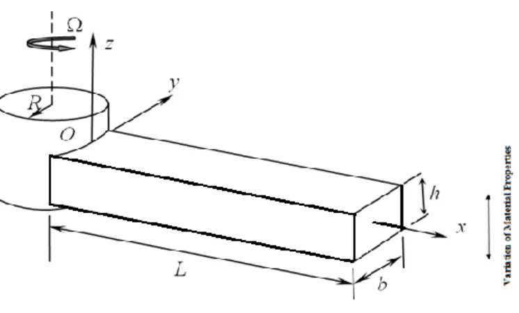
The governing differential equations of motion are derived for the free vibration analysis of a functionally graded rotating Timoshenko beam model with a right-handed Cartesian coordinate system which is represented by Figure 1.
Figure 1. Rotating beam model and coordinate system
Here, a functionally graded Timoshenko beam of length L , which is fixed at point O to a rigid hub with radius 𝑅, is shown. The beam height is h and width is b with cantilever boundary condition at point O. is shown. The 𝑥𝑦𝑧 axes represent a global orthogonal coordinate system with its origin at the root of the beam. The beam is assumed to be rotating in the counter-clockwise direction at a constant angular velocity, Ω. In the right-handed Cartesian coordinate system, the 𝑥 -axis coincides with the neutral axis of the beam in the undeflected position, the 𝑧-axis is parallel to the axis of rotation, but not coincident and the 𝑦-axis lies in the plane of rotation.
FUNCTIONALLY GRADED BEAM FORMULATION Beam Models and Related Formulation
In the present work, flapwise bending vibration analysis of a functionally graded Timoshenko beam that rotates with a constant angular velocity is carried out. The analyses are carried out for two types of FGB models. For the first type, the material properties of the beam vary such that the material at the bottom surface is ceramic and the material at the the top surface is metal as shown in Figure 2(a). For the second type, the beam consists of metallic core with ceramic surfaces as shown in Figure 2(b).
Material properties of the beam, i.e. modulus of elasticity, E, shear modulus, G, Poisson’s ratio, ν and material density, ρ are assumed to vary continuously in the thickness direction, z, as a function of the volume fraction and the properties of the the constituent materials according to a simple power law.
According to the rule of mixture, the effective material property P(z) can be expressed as follows
𝑃(𝑧) = 𝑃𝑐𝑉𝑐+ 𝑃𝑚𝑉𝑚 (1)
where Pc and Pm are the properties of the ceramic and metal while Vc and Vm are the corresponding
volume fractions. The relation between the volume fractions is given by
𝑉𝑚+ 𝑉𝑐= 1 (2)
Beam of The 1st Type (Figure 1a)
The volume fraction of the top constituent of the beam, Vm, is assumed to be given by
𝑉𝑚= (𝑧 ℎ+ 1 2) 𝑘 , (𝑘 ≥ 0) (3)
Here k is the non-negative power law index parameter that dictates the material variation profile through the beam thickness.
Considering Eqns. (1)-(3), the effective material property of the 1st type beam can be rewritten as
follows 𝑃1(𝑧) = (𝑃𝑚− 𝑃𝑐) ( 𝑧 ℎ+ 1 2) 𝑘 + 𝑃𝑐 (4) It is evident from Eqn.(4) that
@ 𝑧 = ℎ 2⁄ , 𝐸 = 𝐸𝑚, 𝜈 = 𝜈𝑚, 𝐺 = 𝐺𝑚, 𝜌 = 𝜌𝑚 (5a)
@ 𝑧 = −ℎ 2⁄ , 𝐸 = 𝐸𝑐, 𝜈 = 𝜈𝑐, 𝐺 = 𝐺𝑐, 𝜌 = 𝜌𝑐. (5b)
Beam of The 2nd Type (Figure 1b)
The volume fraction of the top constituent of the beam, Vt, is assumed to be given by
𝑉𝑐 = [𝑧
ℎ] 𝑘
, (𝑘 ≥ 0) (6)
Considering Eqns. (1), (2) and (6), the effective material property of the 2nd type beam can be rewritten as follows
𝑃2(𝑧) = (𝑃𝑚− 𝑃𝑐) [𝑧
ℎ] 𝑘
+ 𝑃𝑐 (7)
It is evident from Eqn.(7) that
@ 𝑧 = ±ℎ 2⁄ , 𝐸 = 𝐸𝑐, 𝜈 = 𝜈𝑐, 𝐺 = 𝐺𝑐, 𝜌 = 𝜌𝑐. (8a)
@ 𝑧 = 0 , 𝐸 = 𝐸𝑚, 𝜈 = 𝜈𝑚, 𝐺 = 𝐺𝑚, 𝜌 = 𝜌𝑚 (8b)
DISPLACEMENT FIELD AND STRAIN FIELD
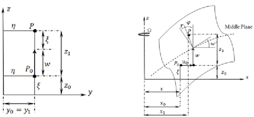
The cross-sectional and the longitudinal views of a Timoshenko beam that undergoes extension and flapwise bending deflections are introduced in Figure 3 (a) and3 (b), respectively. Here, a reference point is chosen and is represented by 𝑃0 before deformation and by 𝑃 after deformation.
Figure 3. (a) Cross-sectional view (b) Longitudinal view of the rotating Timoshenko beam Here, 𝜂 is the offset of the reference point from the z- axis, 𝜉 is the offset of the reference point from the middle plane, 𝑥 is the offset of the reference point from the z-axis, 𝑢0 is the elongation, 𝑤 is the
flapwise bending displacement, 𝜑 is the rotation due to bending and 𝛾 is the shear angle.
Considering Figure 3 (a) and 3 (b), coordinates of the reference point are obtained as follows Before deflection (coordinates of 𝑷𝟎):
𝑥0= 𝑥 (9a)
𝑦0= 𝜂 (9b)
𝑧0= 𝜉 (9c)
After deflection (coordinates of 𝑷):
𝑥1= 𝑥 + 𝑢0+ 𝜉𝜑 (10a)
𝑦1= 𝜂 (10b)
𝑧1= 𝑤 + 𝜉 (10c)
The position vectors of the reference point are represented by 𝑟⃗⃗⃗ and 𝑟0 ⃗⃗⃗ before and after deflection, 1
respectively. Therefore, 𝑑𝑟⃗⃗⃗ and 𝑑𝑟0 ⃗⃗⃗ can be written as follows 1
𝑑𝑟⃗⃗⃗ = 𝑑𝑥𝑖 + 𝑑𝜂𝑗 + 𝑑𝜉𝑘⃗ 0 (11a)
𝑑𝑟⃗⃗⃗ = [(1 + 𝑢1 0′+ 𝜉𝜑′)]𝑑𝑥𝑖 + 𝑑𝜂𝑗 + (𝑤′𝑑𝑥 + 𝑑𝜉)𝑘⃗ (11b)
where ( )′ denotes differentiation with respect to the spanwise coordinate, 𝑥 .
The classical strain tensor 𝜀𝑖𝑗 may be obtained by using the following equilibrium equation given by
Eringen (1980) 𝑑𝑟⃗⃗⃗ . 𝑑𝑟1 ⃗⃗⃗ − 𝑑𝑟1 ⃗⃗⃗ . 𝑑𝑟0 ⃗⃗⃗ = 2[𝑑𝑥0 𝑑𝜂 𝑑𝜉][𝜀𝑖𝑗] [ 𝑑𝑥 𝑑𝜂 𝑑𝜉 ] (12) where [𝜀𝑖𝑗] = [ 𝜀𝑥𝑥 𝜀𝑥𝜂 𝜀𝑥𝜉 𝜀𝜂𝑥 𝜀𝜂𝜂 𝜀𝜂𝜉 𝜀𝜉𝑥 𝜀𝜉𝜂 𝜀𝜉𝜉] (13)
Substituting Eqn. (11a) and Eqn. (11b) into Eqn.(12), the components of the strain tensor 𝜀𝑖𝑗 are
obtained as follows 𝜀𝑥𝑥= 𝑢0′ + (𝑢0′) 2 2 + (𝑤′)2 2 + 𝑢0 ′𝜑′𝜉 + 𝜑′𝜉 +(𝜑′)2 2 𝜉 2 (14a) 𝛾𝑥𝜂= 0 (14b) 𝛾𝑥𝜉= (𝑤′+ 𝜑) + 𝜑𝜑′𝜉 − 𝑢 0 ′𝜑 (14c)
where 𝜀𝑥𝑥, 𝛾𝑥𝜂 and 𝛾𝑥𝜉 are the axial strain and the shear strains, respectively.
In this work; only 𝜀𝑥𝑥, 𝛾𝑥𝜂 and 𝛾𝑥𝜉 are used in the calculations because as noted by Hodges and Dowell
(1974) for long slender beams, the axial strain 𝜀𝑥𝑥 is dominant over the transverse normal strains, 𝜀𝜂𝜂
and 𝜀𝜉𝜉. Moreover, the shear strain 𝛾𝜂𝜉 is two order smaller than the other shear strains, 𝛾𝑥𝜉 and 𝛾𝑥𝜂.
In order to obtain simpler expressions for the strain components given by Eqns. (10a)-(10c), higher order terms can be neglected so an order of magnitude analysis is performed by using the ordering scheme, taken from Hodges and Dowell (1974)and introduced in Table 1.
Table 1. Ordering scheme for the Timoshenko beam model
Term Order 𝑤′ 𝑂(𝜀) 𝜑 𝑂(𝜀) 𝑤′+ 𝜑 𝑂(𝜀2) 𝑢0′ 𝑂(𝜀2) 𝜑′ (𝜀2)
Hodges and Dowell (1974) used the formulation for an Euler-Bernoulli beam so in this study, their formulation is modified for a Timoshenko beam and a new expression, 𝑤′+ 𝜑 = 𝑂(𝜀2) is added to their
ordering scheme as a contribution to literature.
Considering Table 1, Eqns. (14a)-(14c) are simplified as follows 𝜀𝑥𝑥= 𝑢0′ +(𝑢0′) 2 2 + (𝑤′)2 2 + 𝜑 ′𝜉 (15a) 𝛾𝑥𝜂= 0 (15b) 𝛾𝑥𝜉= 𝑤′+ 𝜑 (15c) Potential Energy
The potential energy expression is given by 𝑈 =1 2∫ ∫ (𝜎𝑥𝑥𝜀𝑥𝑥+ 𝜏𝑥𝜉𝛾𝑥𝜉)𝑑𝐴 𝑑𝑥 = 𝑏 2∫ ∫ (𝜎𝑥𝑥𝜀𝑥𝑥+ 𝜏𝑥𝜉𝛾𝑥𝜉)𝑑𝜉 𝑑𝑥 ℎ 2 ⁄ −ℎ 2⁄ 𝐿 0 𝐴 𝐿 0 (16)
The axial force, N, the bending moment, M and the shear force, Q that act on a laminate at the midplane are expressed as follows (Kollar and Springer, 2003)
𝑁 = 𝑏 ∫ℎ⁄2 𝜎𝑑𝑧 −ℎ 2 ⁄ (17a) 𝑀 = 𝑏 ∫ℎ⁄2 𝑧𝜎𝑑𝑧 −ℎ 2 ⁄ (17b) 𝑄 = 𝑏 ∫−ℎℎ⁄2 𝜏𝑑𝑧 2 ⁄ (17c)
Substituting Eqns. (15a)-(15c) into Eqn. (16) and considering Eqns. (17a)-(17c), the following expression is obtained. 𝑈 =1 2∫ {𝑁𝑥[𝑢0 ′+(𝑤′) 2 2 ] + 𝑀𝑥𝜑 ′+ 𝑄 𝑥𝑧(𝑤′+ 𝜑 )} 𝐿 0 (18) where 𝑁𝑥 = 𝐴̅11𝑢0′ + 𝐵̅11𝜑′ (19a) 𝑀𝑥= 𝐵̅11𝑢0′+ 𝐷̅11𝜑′ (19b) 𝑄 = 𝐴̅55𝛾𝑥𝜉 (19c)
Here the stiffness coefficients are obtained as follows [𝐴̅11 𝐵̅11 𝐷̅11] = ∫ 𝐸(𝑧) [1 𝑧 𝑧2]
𝐴 𝑑𝐴 (20a)
𝐴̅55= 𝐾 ∫ 𝐺(𝑧) 𝑑𝐴𝐴 (20b)
where K is defined as the shear correction factor that takes the value of 𝐾 = 5 6⁄ for rectangular cross sections.
Substituting Eqns. (19a)-(19c) into Eqn. (18) gives 𝑈 =1 2∫ {𝐴̅11(𝑢0 ′)2+ 2𝐵̅ 11𝑢0′𝜑′+ 𝐷̅11(𝜑′)2+ 𝐴̅55(𝑤′+ 𝜑 )}𝑑𝑥 𝐿 0 (21)
The uniform strain, 𝜀0, and the associated axial displacement, 𝑢0, due to the centrifugal force, 𝑇(𝑥),
𝑢0′ = 𝜀 0=
𝑇(𝑥)
𝐴̅11 (22)
where the centrifugal force, 𝑇(𝑥), is expressed by 𝑇(𝑥) = ∫ 𝜌𝐴(𝑅 + 𝑥)Ω𝐿 2
𝑥 𝑑𝑥 (23)
Here 𝜌 is the material density and 𝐴 is the cross-sectional area.
Referring to the Eqns. (17)-(18), variation of Eqn. (17) is obtained as follows. 𝛿𝑈 = ∫ {(𝐴̅11𝑢0′+ 𝐵̅11𝜑′)𝛿𝑢0′+ (𝐵̅11𝑢0′+ 𝐷̅11𝜑′)𝛿𝜑′+ 𝐴̅55(𝑤′+ 𝜑 )(𝛿𝑤′+ 𝛿𝜑)}𝑑𝑥
𝐿
0 (24)
Kinetic Energy
The position vector of point P shown in Figure 3 is given by
𝑟 = (𝑥 + 𝑢0+ 𝜉𝜑)𝑖 + 𝑤𝑘⃗ (25a)
The velocity vector of this point due to rotation of the beam is obtained as follows 𝑉⃗ =𝜕𝑟
𝜕𝑡+ Ω𝑘⃗ × 𝑟 = (𝑢̇0+ 𝜉𝜑̇)𝑖 + (𝑅 + 𝑥 + 𝑢0+ 𝜉𝜑)Ω𝑗 + 𝑤̇𝑘⃗ (25b)
Hence, the velocity components are
𝑉𝑥 = 𝑢̇0+ 𝜉𝜑̇ (26a)
𝑉𝑦= (𝑅 + 𝑥 + 𝑢0+ 𝜉𝜑)Ω (27b)
𝑉𝑧= 𝑤̇ (28c)
The kinetic energy expression is given by 𝐾 =1 2∫ ∫ 𝜌(𝑉𝑥 2+ 𝑉 𝑦2+ 𝑉𝑧2) 𝑑𝐴 𝑑𝑥 = 𝑏 2∫ ∫ 𝜌(𝑉𝑥 2+ 𝑉 𝑦2+ 𝑉𝑧2) ℎ 2 ⁄ −ℎ 2 ⁄ 𝐿 0 𝑑𝜉 𝑑𝑥 𝐴 𝐿 0 (29)
Substituting the velocity components into Eq. (29) and taking the variation of the kinetic energy give
(30) where 𝐼1, 𝐼2 and 𝐼3 are the inertial characteristics of the beam given by
[𝐼1 𝐼2 𝐼3] = ∫ 𝜌(𝑧) [1 𝑧 𝑧𝐴 2] 𝑑𝐴 (31)
Equations of Motion and The Boundary Conditions The Hamilton’s Principle is expressed as follows
∫ 𝛿(𝑈 − 𝐾)𝑑𝑡 = 0𝑡1𝑡2 (32)
Substituting Eqn.(24) and Eqn.(30) into Eqn. (32) gives the equations of motion and the boundary conditions as follows Equations of Motion: 𝐴̅11𝑢0′′+ 𝐵̅ 11𝜑′′+ 𝐼1Ω2 𝑢0 + 𝐼2Ω2 𝜑 = 𝐼1𝑢̈0+ 𝐼2𝜑̈ (33a) (𝑤′𝑇)′+ (𝐴̅ 55− 𝐸̅11)𝑤′′+ 𝐴̅55𝜑′= 𝐼1𝑤̈ (33b) 𝐷̅11𝜑′′+ 𝐵̅11𝑢0′′+ 𝐼2Ω2 𝑢0 + 𝐼3Ω2 𝜑 − 𝐴̅55(𝑤′+ 𝜑) = 𝐼2𝑢̈0+ 𝐼3𝜑̈ (33c)
where the expression of the centrifugal force, 𝑇, given by Eq. (23) can be rewritten as follows 𝑇(𝑥) = ∫ 𝐼1(𝑅 + 𝑥)Ω2
𝐿
𝑥 𝑑𝑥 (34)
Clamped-Free Boundary Conditions:
@ 𝑥 = 0 𝑢0(0, 𝑡) = 𝑤(0, 𝑡) = 𝜑(0, 𝑡) = 0 (35a) @ 𝑥 = 𝐿 𝐴̅11𝑢0′(𝐿, 𝑡) + 𝐵̅11𝜑′(𝐿, 𝑡) = 0 (35b) 𝑇𝑤′(𝐿, 𝑡) + 𝐴̅ 55[𝑤′(𝐿, 𝑡) + 𝜑(𝐿, 𝑡)] = 0 (35c) 𝐷̅11𝜑(𝐿, 𝑡) + 𝐵̅11𝑢0′(𝐿, 𝑡) − 𝐴̅ 55(𝑤′+ 𝜑) = 0 (35d)
The boundary condition expressed by Eq. (35c) can be written in a simpler form by noting that the centrifugal force is zero at the free end of the beam, T
L 0.𝐴̅55[𝑤′(𝐿, 𝑡) + 𝜑(𝐿, 𝑡)] = 0 (36)
In order to investigate the free vibration of the beam model considered in this study, a sinusoidal variation of 𝑢0, 𝑤 and 𝜑 with a circular natural frequency, 𝜔, is assumed and the functions are
approximated as
𝑢0(𝑥, 𝑡) = 𝑢̅(𝑥)𝑒𝑖𝜔𝑡 (37a)
𝑤(𝑥, 𝑡) = 𝑤̅(𝑥)𝑒𝑖𝜔𝑡 (37b)
𝜑(𝑥, 𝑡) = 𝜑̅(𝑥)𝑒𝑖𝜔𝑡 (37c)
Substituting Eqns. (37a)-(37c) into the equations of motion, i.e. Eqns.(33a)-(33c), and into the boundary conditions, i.e. Eqns.(35a)-(35d), the following dimensionless equations are obtained as follows
Equations of motion:
γ2ũ∗∗+ α2φ̃∗∗+ (β2+ λ2) (ũ + 𝜇2φ̃) = 0 (38a)
{β2[σ(1 − x̅) +1 2 (1 − x̅ 2)] + 1 τ2− e0} w̃∗∗− β2(σ + x̅)w̃∗+ λ2w̃ + 1 τ2φ̃∗= 0 (38b) α2τ2ũ∗∗+ τ2φ̃∗∗+ 𝜇2τ2(β2+ λ2)ũ + [r2τ2(β2+ λ2) − 1]φ̃ − w̃∗= 0 (38c)
Clamped-Free Boundary Conditions: @ 𝑥̅ = 0 ũ(0, 𝑡) = w̃ (0, 𝑡) = φ̃(0, 𝑡) = 0 (39a) @ 𝑥̅ = 1 γ2ũ∗(𝐿, 𝑡) + α2φ̃∗(𝐿, 𝑡) = 0 (39b) (1 τ2− e0) w̃∗(𝐿, 𝑡) + 1 τ2φ̃(𝐿, 𝑡) = 0 (39c) 𝛼2ũ∗(𝐿, 𝑡) + φ̃∗(𝐿, 𝑡) = 0 (39d)
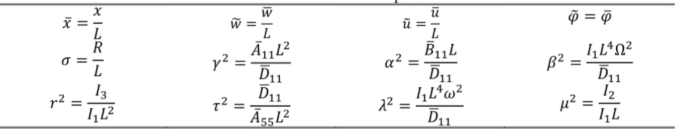
Here, the dimensionless parameters given below in Table 2, are used to be able to simplify the equations of motion, boundary conditions and to make comparisons with open literature.
Table 2. Dimensionless parameters 𝑥̅ =𝑥 𝐿 𝑤̃ = 𝑤̅ 𝐿 𝑢̃ = 𝑢̅ 𝐿 𝜑̃ = 𝜑̅ 𝜎 =𝑅 𝐿 𝛾2= 𝐴̅11𝐿2 𝐷̅11 𝛼2=𝐵̅11𝐿 𝐷̅11 𝛽2=𝐼1𝐿 4Ω2 𝐷̅11 𝑟2= 𝐼3 𝐼1𝐿2 𝜏 2= 𝐷̅11 𝐴̅55𝐿2 𝜆2=𝐼1𝐿 4𝜔2 𝐷̅11 𝜇2= 𝐼2 𝐼1𝐿
where 𝛽 is the rotational speed parameter, 𝜆 is the frequency parameter, 𝑟 is the inverse of the slenderness ratio and 𝜎 is the hub radius parameter.
DIFFERENTIAL TRANSFORM METHOD
The Differential Transform Method (DTM) is a transformation technique based on the Taylor series expansion and is a useful tool to obtain analytical solutions of the differential equations. In this method, certain transformation rules are applied and the governing differential equations and the boundary conditions of the system are transformed into a set of algebraic equations in terms of the differential transforms of the original functions and the solution of these algebraic equations gives the desired solution of the problem.
Consider a function f
x which is analytic in a domain D and letx
x
0 represent any point in D. The functionf
x
is then represented by a power series whose center is located atx
0. The differential transform of the functionf
x
is given by
0 ) ( ! 1 x x k k dx x f d k k F (40)where
f
x
is the original function andF
k
is the transformed function. The inverse transformation is defined as
0 0) ( ) ( k kF k x x x f (41)Combining Eqn. (40) and Eqn. (41), we get
0 0 0 ) ( ! ) ( ) ( k x x k k k dx x f d k x x x f (42)Considering Eqn. (42), it is noticed that the concept of differential transform is derived from Taylor series expansion. However, the method does not evaluate the derivatives symbolically.
In actual applications, the function
f
x
is expressed by a finite series and Eqn. (42) can be written as follows
m k x x k k k dx x f d k x x x f 0 0 0 ) ( ! ) ( ) ( (43)which means that the rest of the series
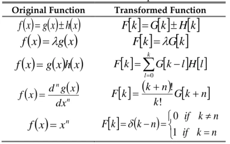
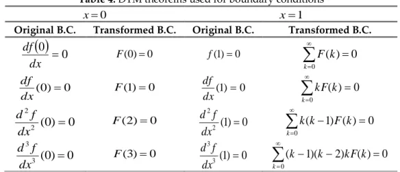
1 0 0 ) ( ! ) ( ) ( m k x x k k k dx x f d k x x x f (44)is negligibly small. Here, the value of 𝑚 depends on the convergence of the natural frequencies. Theorems that are frequently used in the transformation procedure are introduced in Table 3 and theorems that are used for boundary conditions are introduced in Table 4.
Table 3. DTM theorems used for equations of motion Original Function Transformed Function
x
g
x
h
x
f
F
k
G
k
H
k
x
g
x
f
F
k
G
k
x
g
x
h
x
f
k ll
H
l
k
G
k
F
0
n
ndx
x
g
d
x
f
G
k
n
k
n
k
k
F
!
!
nx
x
f
n
k
if
n
k
if
n
k
k
F
1
0
Table 4. DTM theorems used for boundary conditions 0
x x1
Original B.C. Transformed B.C. Original B.C. Transformed B.C.
0
0
dx
df
0 ) 0 ( F f(1)0
00
)
(
kk
F
0 ) 0 ( dx df 0 ) 1 ( F (1)0 dx df
00
)
(
kk
kF
0
)
0
(
2 2
dx
f
d
F(2)00
)
1
(
2 2
dx
f
d
00
)
(
)
1
(
kk
F
k
k
0
)
0
(
3 3
dx
f
d
F(3)00
)
1
(
3 3
dx
f
d
00
)
(
)
2
)(
1
(
kk
kF
k
k
After applying the differential transform method to Eqns. (38a)-(39d), the transformed equations of motion and boundary conditions are obtained as follows
Equations of motion: 𝛾2(𝑘 + 1)(𝑘 + 2)𝑈[𝑘 + 2] + 𝛼2(𝑘 + 1)(𝑘 + 2)𝜑[𝑘 + 2] + (𝛽2+ 𝜆2) (𝑈[𝑘] + 𝜇2𝜑[𝑘]) = 0 (45a) (45b) 𝛼2(𝑘 + 1)(𝑘 + 2)𝑈[𝑘 + 2] + (𝑘 + 1)(𝑘 + 2)𝜑[𝑘 + 2] + 𝜇2(𝛽2+ 𝜆2)𝑈[𝑘] + [𝑟2(𝛽2+ 𝜆2) − 1 𝜏2] 𝜑[𝑘] − 1 𝜏2(𝑘 + 1)𝑊[𝑘 + 1] = 0 (45c)
Clamped-Free Boundary Conditions:
@ 𝑥̅ = 0 𝑈[𝑘] = 𝑊[𝑘] = 𝜑[𝑘] = 0 (46a) @ 𝑥̅ = 1 γ2∑∞ k𝑈[𝑘] k=0 + α2∑∞k=0k𝜑[𝑘]= 0 (46b) (1 τ2− e0) ∑ k𝑊[𝑘] ∞ k=0 + 1 τ2∑ 𝜑[𝑘] ∞ k=0 = 0 (47c) 𝛼2∑∞ k𝑈[𝑘] k=0 + ∑∞k=0k𝜑[𝑘]− f0= 0 (48d)
RESULTS AND DISCUSSIONS
In numerical analysis, effects of several parameters, i.e. material distribution property, angular velocity, Ώ, , slenderness ratio, L/h and power law index parameter, k, on the natural frequencies of a FG Timoshenko beam are investigated and the results are presented in related tables. In order to validate the calculated results, comparisons with the studies in open literature are made. It is believed that the tabulated results can be used as references by the other researchers to validate their results.
Material Properties
As in the work of Şimsek (2010), Aluminum (Al) is used as the metal and Alumina (Al2O3) is used
Table 5. Material properties of the FG beam
Property Aluminum (Al) Alumina (Al2O3)
Elasticity Modulus, 𝐄 70 GPa 380 GPa
Material Density, 𝛒 2702 kg/m3 3960 kg/m3
Poisson’s Ratio, 𝛎 0.3 0.3
Variation of the fundamental natural frequency of a nonrotating C-F Functionally Graded Timoshenko Beam according to the power law exponent for L/h=20 is introduced in Table 6. The dimensionless frequency values are given by the formula, 𝝀 =𝝎𝑳𝒉𝟐√𝝆𝑬𝒎
𝒎 .
The calculated results of a nonrotating FG Timoshenko beam are compared with the ones given by Şimsek (2010), a very good agreement between the results is observed
.
Table 6. Dimensionless fundamental frequencies of a nonrotating C-F FG timoshenko beam
Frequency Power Law Exponent (k)
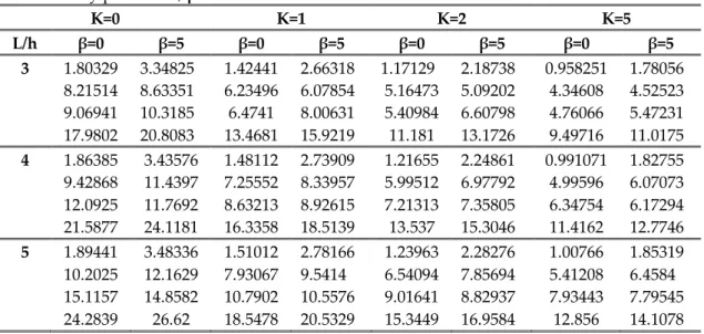
𝝀 =𝝎𝑳 𝟐 𝒉 √ 𝝆𝒎 𝑬𝒎 0 0.2 0.5 1 2 5 10 Full Metal Fundamental 1.94955 1.81407 1.66026 1.50103 1.36966 1.30373 1.26493 1.01297 Şimsek (2010) 1.94957 1.81456 1.66044 1.50104 1.36968 1.30375 1.26495 1.01297 In Table 7, variation of the dimensionless natural frequencies of a C-F Functionally Graded Timoshenko Beam with respect to the power law exponent, k, the slenderness ratio, L/h and the rotational velocity parameter, β is introduced for the beam model where the material properties vary such that the material at the bottom surface is ceramic and the material at the the top surface is metal as shown in Figure 2(a).
Table 7. Variation of the dimensionless natural frequencies of a C-F functionally graded rotating timoshenko beam with respect to the power law exponent, k, the slenderness ratio, L/h and the rotational velocity parameter, β where 𝑃1(𝑧) = (𝑃𝑚− 𝑃𝑐) (
𝑧 ℎ+ 1 2) 𝑘 + 𝑃𝑐 K=0 K=1 K=2 K=5 L/h β=0 β=5 β=0 β=5 β=0 β=5 β=0 β=5 3 1.80329 3.34825 1.39885 2.7451 1.27348 2.58828 1.19956 2.41723 8.21514 8.63351 6.44425 7.11864 5.77913 6.34967 5.22620 5.47542 9.06941 10.3185 7.7081 8.47941 7.05971 7.91179 6.19459 7.28635 17.9802 20.8083 14.3438 16.6267 12.9094 15.0887 11.6647 13.7449 4 1.86385 3.43576 1.44141 2.8159 1.31344 2.65917 1.24242 2.4888 9.42868 11.4397 7.39468 9.02089 6.68493 8.18294 6.15895 7.32402 12.0925 11.7692 10.1889 10.0519 9.27327 9.25019 8.07187 8.28298 21.5877 24.1181 17.1413 19.2664 15.4804 17.5649 14.1093 16.1152 5 1.89441 3.48336 1.46276 2.85363 1.33353 2.69678 1.26419 2.52732 10.2025 12.1629 7.97167 9.67831 7.23018 8.90268 6.72424 8.2538 15.1157 14.8582 12.7061 12.5178 11.5406 11.3768 10.0258 9.89435 24.2839 26.62 19.1875 21.1936 17.3683 19.3554 15.9509 17.851 In Table 8, variation of the dimensionless natural frequencies of a C-F Functionally Graded Timoshenko Beam with respect to the power law exponent, k, the slenderness ratio, L/h and the rotational velocity parameter, β is introduced for the beam model that consists of metallic core with ceramic surfaces as shown in Figure 2(b) where 𝑃2(𝑧) = (𝑃𝑚− 𝑃𝑐) [
𝑧 ℎ]
𝑘
Table 8. Variation of the dimensionless natural frequencies of a C-F Functionally Graded Rotating Timoshenko Beam with respect to the power law exponent, k, the slenderness ratio, L/h and the rotational velocity parameter, β where 𝜎 = 0.
K=0 K=1 K=2 K=5 L/h β=0 β=5 β=0 β=5 β=0 β=5 β=0 β=5 3 1.80329 3.34825 1.42441 2.66318 1.17129 2.18738 0.958251 1.78056 8.21514 8.63351 6.23496 6.07854 5.16473 5.09202 4.34608 4.52523 9.06941 10.3185 6.4741 8.00631 5.40984 6.60798 4.76066 5.47231 17.9802 20.8083 13.4681 15.9219 11.181 13.1726 9.49716 11.0175 4 1.86385 3.43576 1.48112 2.73909 1.21655 2.24861 0.991071 1.82755 9.42868 11.4397 7.25552 8.33957 5.99512 6.97792 4.99596 6.07073 12.0925 11.7692 8.63213 8.92615 7.21313 7.35805 6.34754 6.17294 21.5877 24.1181 16.3358 18.5139 13.537 15.3046 11.4162 12.7746 5 1.89441 3.48336 1.51012 2.78166 1.23963 2.28276 1.00766 1.85319 10.2025 12.1629 7.93067 9.5414 6.54094 7.85694 5.41208 6.4584 15.1157 14.8582 10.7902 10.5576 9.01641 8.82937 7.93443 7.79545 24.2839 26.62 18.5478 20.5329 15.3449 16.9584 12.856 14.1078 In this study, formulation of a rotating functionally graded Timoshenko beam that undergoes flapwise bending vibration is derived by introducing several explanotary figures and tables. Applying the Hamilton’s Principle to the obtained energy expressions, governing differential equations of motion and the boundary conditions are derived. In the solution part, the equations of motion, including the parameters for the rotary inertia, shear deformation, power law index parameter, material distribution, slenderness ratio and rotational speed are solved using an efficient mathematical technique, called the Differential Transform Method (DTM). Natural frequencies are calculated and effects of the parameters,mentioned above, are investigated.
Considering the calculated results, the following conclusions are reached: a. As the slenderness ratio L/h increases, the natural frequencies increase;
b. As the rotational speed parameter increases, the natural frequencies increase due to the stiffening effect of the centrifugal force.
c. The natural frequencies decrease as the value of the power-law exponent, k, increases for both types of beam models.
d. When Table 7 and Table 8 are compared, it is noticed that natural frequencies of the first beam model , i.e. the material properties vary such that the material at the bottom surface is ceramic and the material at the the top surface is metal, are higher than the natural frequencies of the second beam model, i.e. consists of metallic core with ceramic surfaces.
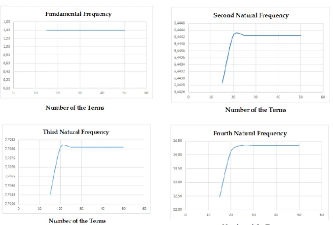
In Figure 4, convergence of the first five natural frequencies with respect to the number of terms, N, used in DTM application is introduced where L/h=3 and k=1. To evaluate up to the fifth natural frequency to fourth-digit precision, it was necessary to take 45 terms. During the calculations, it is noticed that when the rotational speed parameter is increased, the number of the terms has to be increased to achieve the same accuracy. Additionally, here it is seen that higher modes appear when more terms are taken into account in DTM application. Thus, depending on the order of the required mode, one must try a few values for the term number at the beginning of the calculations in order to find the adequate number of terms. For instance, only N=100 is enough for the results given in Table 7 and Table 8.
Figure 4. Convergence of the first five natural frequencies with respect to the number of terms, N REFERENCES
Akash, B. A., Mamlook, R., Mohsen, S. M., 1999, “Multi-criteria selection of electric power plants using analytical hierarchy process”, Electric Power Systems Research, Cilt 52, Sayı 1, ss. 29-35.
Alshorbagy AE, Eltaher MA, Mahmoud FF, 2011, Free vibration characteristics of a functionally graded beam by finite element method, Applied Mathematical Modelling, 35, 412–425.
Bhimaraddi A, Chandrashekhara K., 1991, Some observation on the modeling of laminated composite beams with general lay-ups, Composite Structures, 19, 371–380
Chakraborty A, Gopalakrishnan S, Reddy JN., 2003, A new beam finite element for the analysis of functionally graded materials, International Journal of Mechanical Sciences, 45, 519–539.
Dadfarnia M., 1997, Nonlinear forced vibration of laminated beam with arbitrary lamination, M.Sc. Thesis, Sharif University of Technology.
Deng HD and Wei C, 2016, Dynamic characteristics analysis of bi-directional functionally graded Timoshenko beams, Composite Structures, in press.
Eringen, AC., 1980, Mechanics of Continua, Robert E. Krieger Publishing Company, Huntington, New York.
Giunta G, Crisafulli D, Belouettar S, Carrera E., 2011, Hierarchical theories for the free vibration analysis of functionally graded beams, Composite Structures, 94, 68–74.
Hodges, D. H., Dowell, E. H., 1974, Nonlinear equations of motion for the elastic bending and torsion of twisted nonuniform rotor blades, NASA Technical Report,NASA TN D-7818.
Huang Y, Li XF., 2010, A new approach for free vibration of axially functionally graded beams with non-uniform cross-section, Journal of Sound and Vibration, 329, 2291–2303.
Kapuria S, Bhattacharyya M, Kumar AN., 2008, Bending and free vibration response of layered functionally graded beams: a theoretical model and its experimental validation, Composite Structures, 82, 390–402.
Kaya, M.O., Ozdemir Ozgumus, O., 2007, Flexural–torsional-coupled vibration analysis of axially loaded closed-section composite Timoshenko beam by using DTM, Journal of Sound and Vibration, 306, 495–506.
Kaya, M.O., Ozdemir Ozgumus, O., 2010, Energy expressions and free vibration analysis of a rotating uniform timoshenko beam featuring bending–torsion coupling, Journal of Vibration and Control, 16(6), 915–934.
Kollar, LR., Springer, GS., 2003, Mechanics of Composite Structures. Cambridge University Press, United Kingdom.
Lai SK, Harrington J, Xiang Y, Chow KW., 2012, Accurate analytical perturbation approach for large amplitude vibration of functionally graded beams, International Journal of Non-Linear Mechanics, 47, 473–480.
Li XF., 2008, A unified approach for analyzing static and dynamic behaviors of functionally graded Timoshenko and Euler–Bernoulli Beams, Journal of Sound and Vibration, 318, 1210–1229.
Li XF, Kang YA, Wu JX, 2013, Exact frequency equation of free vibration of exponentially funtionally graded beams, Applied Acoustics, 74 (3), 413-420.
Loja MAR, Barbosa JI, Mota Soares CM., 2012, A study on the modelling of sandwich functionally graded particulate composite, Composite Structures, 94, 2209–2217.
Loy C.T., Lam K.Y., Reddy J.N., 1999, Vibration of functionally graded cylinderical shells, International Journal of Mechanical Science, 41, 309-324.
Lu CF, Chen WQ., 2005, Free vibration of orthotropic functionally graded beams with various end conditions, Structural Engineering and Mechanics, 20, 465–476.
Ozdemir O., 2016, Application of The Differential Transform Method to The Free Vibration Analysis of Functionally Graded Timoshenko Beams, Journal of Theoretical and Applied Mechanics
54, 4, 1205-1217.
Ozdemir Ozgumus, O., Kaya, M.O., 2013, Energy expressions and free vibration analysis of a rotating Timoshenko beam featuring bending–bending-torsion coupling, Archive of Applied Mechanics, 83, 97–108.
Sina S.A., Navazi H.M., Haddadpour H., 2009, An analytical method for free vibration analysis of functionally graded beams, Materials and Design, 30, 741–747.
Şimsek M., 2010, Fundamental frequency analysis of functionally graded beams by using different higher-order beam theories, Nuclear Engineering and Design, 240, 697–705.
Tang AY, Wu JX, Li XF and Lee KY, 2014, Exact frequency equations of free vibration of exponentially non-uniform functionally graded Timoshenko beams, International Journal of Mechanical Sciences, 89, 1-11.
Thai HT, Vo TP., 2012, Bending and free vibration of functionally graded beams using various higher-order shear deformation beam theories, International Journal of Mechanical Sciences, 62, 57–66.
Wang Z., Wang X., Xu G., Cheng S. and Zeng T., 2016, Free vibration of two directional functionally graded beams, Composite Structures, 135, 191-198.
Wattanasakulpong N, Prusty BG, Kelly DW, Hoffman M., 2012, Free vibration analysis of layered functionally graded beams with experimental validation, Materials & Design, 36, 182–190. Zhong Z, Yu T., 2007, Analytical solution of a cantilever functionally graded beam, Composites Science