Network Traffic Prediction Using Variational
Mode Decomposition and
Multi-Reservoirs Echo State Network
YING HAN1,2, YUANWEI JING1, KUN LI 2, AND GEORGI MARKO DIMIROVSKI3,4 1College of Information Science and Engineering, Northeastern University, Shenyang 110819, China
2College of Engineering, Bohai University, Jinzhou 121013, China 3School of Engineering Department, Dogus University, 34722 Istanbul, Turkey 4School FEIT, Saints Cyril and Methodius University of Skopje, 1000 Skopje, Macedonia Corresponding author: Kun Li ([email protected])
This work was supported in part by the National Natural Science Foundation of China under Grant 61773108 and Grant 61403040, and in part by the Fund for Science of Dogus University.
ABSTRACT The network traffic prediction is significant for the network load pre-warning and network congestion control. But the nonlinearity and nonstationarity of the actual network traffic data would reduce the prediction accuracy. In this paper, an optimized network traffic prediction method using variational mode decomposition (VMD) and multi-reservoirs echo state network (ESN) is presented. VMD method has advantages of reducing the signal transmission errors, removing the mode aliasing, and decreasing the degree of endpoint effects. However, VMD needs to preset the number of modes and the iterative factor, which are mainly decided by subjective experiences. In order to solve this, an optimized VMD method is proposed, and then a multi-reservoirs echo state network based prediction model is constructed. The main works are as follows: First, VMD is used to decompose the original network traffic data into several subsets; then, multiple subreservoirs are built after the phase space reconstruction (PSR) of each data subset; finally, the training set is used to train the prediction model. Moreover, in the training process, an improved fruit fly optimization algorithm (IFOA) is proposed combined with the levy’s flight function and the cloud generator, which is used to optimize some model parameters. Compared with several prediction models, the proposed VMD-IFOA-ESN has better predictive stability and convergence performance. Three WIDE backbone network traffic data sets with different time intervals verify the effectiveness of the proposed prediction model.
INDEX TERMS Echo state network, fruit fly optimization algorithm, multiple reservoirs, network traffic prediction, time series analysis, variational modal decomposition.
I. INTRODUCTION
With the rapid development of the internet scale, the number of users are increasing (like the smartphone, the mobile video, the ‘‘Internet of Things’’ connection), which makes the net-work traffic data have a substantial growth and also increase frequency of the network congestion. It is essential to use time series analysis to do accurate network traffic prediction by a prediction model, namely, the continuous changes of data characteristics in a certain period of time is used to predict the future states of the system. Now, many methods have been used for the network traffic prediction model,
The associate editor coordinating the review of this manuscript and approving it for publication was Varuna De Silva .
such as: least square support vector machine (LSSVM) [1], Elman neural network [2], finite impulse response neural network (FIRNN) [3], extreme learning machine (ELM) [4], radial basis function neural network (RBFNN) [5], echo state network (ESN) [6], etc. LSSVM is a statistic learning method based on small samples which has simple structure, however, its prediction results are greatly affected by different kernel function types and kernel parameter values; Elman neural network uses the estimation of error gradient in the training phase, which makes the poor reliability; ELM has advantages of high learning efficiency and strong generalization ability, however, more hidden layer nodes increase the computational burden, and prone to the over-fitting problem; FIRNN has complex calculation, and it is easy to fall into the local
extremum; RBFNN is an improvement of BP neural net-work, however, it has poor generalization ability. ESN is a type of recursive neural network, which is mainly used for time series analysis. It has a dynamic reservoir with large scale, includes: input units, internal units and output units. Four weights matrixes are mainly used for model calculation, respectively are: the input weight matrix from input units to internal units of the reservoir, the internal weight matrix of all the weight between internal units, the feedback weight matrix from output units back to internal units, and the output weight matrix from input units and internal units to output units. In the initialization phase, the input weight matrix, the internal weight matrix and the feedback weight matrix are randomly generated and remain unchanged during the training process; only the output weight matrix needs to be trained. Therefore, compared with some other neural network based learning methods, ESN has simple algorithm structure, less computation and better generalization ability, which has been widely used in many fields [7]–[10].
The randomness and non-stationarity properties of the actual network traffic data make the network traffic time series have strong nonlinearity. Thus, complex data changing rules will produce larger prediction errors. To solve this prob-lem, ESN ensemble modeling methods based on time-series decomposition have been paid attention to. For multivariate time series prediction problems, a multi-reservoirs echo state network model based on sparse bayesian learning algorithm was proposed by Han and Mu [11], which can solve the problem that only single phase space reconstructed parameter can be used in a single reservoir. In [12], Rabin et al. used a linear learning method based on the nonlinear monotone function to build a multi-reservoirs echo state network model, which has better prediction performance than single reservoir. Lv et al. [13] proposed an ESN ensemble modeling method based on quantile regression (QR), which builds one reservoir for each group samples after using the QR method to divide the original data set into many subsets and then output an integrate result. For the problem of prognostics and health management (PHM), Zhong et al. [9] proposed an echo state network model with two reservoirs, of which one reservoir is used to build model of the sensor data sequence and the other is used to build model of the state parameter data sequence. In [14], Qiao et al. proposed a growing echo state network model with multiple subreservoirs which is used to solve the coupling problem among different units. From the above, compared with the single reservoir, the multi-reservoirs method can effectively deal with data sequences with different time scales and reduce coupling among dif-ferent units. On the basis of this, in this paper, the origi-nal network traffic data is firstly decomposed into sub-data sequences with different time scales; then, for each sub-data sequence, one reservoir is modeled; finally, ensemble results of multiple reservoirs are output.
Time-series decomposition (TSD) analysis [15] is an effec-tive method to deal with the nonlinearity and nonstationarity of the data sequence. In this paper, TSD method is used to
build multiple subreservoirs. The original signal is decom-posed into various signal components with different time scales, and then one subreservoir is constructed for each signal component; thus, the original signal will not be pro-cessed by single reservoir with uniform structural parame-ters, but respectively be processed by multiple subreservoirs with different structural parameters, which will increase the adaptive ability of the prediction model to the actual net-work traffic data. Now, there are many commonly used TSD methods, for instance, wavelet decomposition (WD), empir-ical mode decomposition (EMD), ensemble empirempir-ical mode decomposition (EEMD), complementary ensemble empirical mode decomposition (CEEMD), local mean decomposition (LMD), variational mode decomposition (VMD), etc. In [16], WD was used to carry out multi-scale analysis for the data sequence by dilation and translation operations, which ulti-mately achieves time breakdowns in the high frequency and frequency breakdowns in the low frequency; however, it has uncertain decomposition results because selection of wavelet basis function and optimal threshold value is easily influ-enced by many subjective factors. EMD [17] was proposed to decompose the nonstationary data sequence into a finite number of intrinsic mode functions (IMF), which contains local features of the original signal at different time scales; however, EMD is easily influenced by mode aliasing and noise interference. In [18], on the basis of EMD, EEMD was proposed to remove the mode aliasing, which added different random white noise to the original data sequence to map signal regions with different scales to appropriate scales asso-ciated with the white noise; however, these white noises could increase the error of data reconstruction because they could not be completely neutralized. CEEMD [19] was proposed to improve the EEMD, which added random paired white noises with opposite values to the original data sequence to balance the random errors; however, it needs large amount of computation. In [20], LMD was proposed to adaptively decompose the original data sequence according to its own information, which can reflect the distribution law of signal energy in each scale by producing various product functions (PF) with real physical meanings; however, it has some dis-advantages by too many smoothing times make the signal have lag or advance, uncertainty of the best smoothing step. VMD [21] was a new non-recursive signal decomposition method, which was used to transform the signal decom-position problem into a constrained optimization problem; it can reduce signal transmission errors, remove the mode aliasing, and decrease degree of endpoint effects. The VMD method is used to preprocess the original network traffic data sequence, which needs to preset the number of modes K and the iterative factorτ. Compared with the manual way, parameter selection based on the swarm intelligence opti-mization algorithm can better adapt to data sets with different distributions, for instance, firefly algorithm (FA) [22], gravi-tational search algorithm (GSA) [15], grey wolf optimization (GWO) [23]. Fruit fly optimization algorithm (FOA) [24] was proposed by Pan in the year 2012, which had less subjective
parameters, simple programming and better convergence speed; it has been widely used in many research fields [22], [25]–[28]. In order to decrease randomness and fuzziness during individual flight, Wu et al. [29] proposed an improved FOA based on cloud model. It used an adaptive mechanism to define search radius following the change of iterations, that larger search radius in the early stage of iterations to find the optimal solution, and smaller search radius in the late stage of iterations to approach the optimal solution. How-ever, it still has deficiencies of increasing population diver-sity and easily jumping out of the local optimum. To solve these, an improved cloud model based FOA (IFOA) is pro-posed in this paper to optimize several model parameters, which has a combination of cloud model and Levy’s flight function.
Our major contributions are summarized as follows: (1) An optimized VMD method was proposed in this paper, in which the optimal value of the number of modes and the iterative factor is automatically deter-mined, replacing that they are decided by subjective experiences;
(2) An echo state network model with multiple subreser-voirs was automatically built according to the optimized decomposition results by VMD;
(3) An improved fruit fly optimization algorithm combined with the cloud model and the levy flight function was pro-posed to optimize several model parameters;
(4) An integrated model based on VMD, multi-reservoirs ESN, PSR and IFOA was proposed for network traffic prediction.
The rest of this paper is organized as follows. Section 2 briefly introduces main steps of VMD. In Section 3, structure of the multi-reservoirs echo state network is designed. PSR method is introduced in Section 4, which is used to reconstruct each data subset after signal decom-position; and then, both inputs and outputs after PSR are used for multi-reservoirs echo state network. The proposed prediction model is introduced in Section 5, of which Sub-section 5.1 introduces basic structure of the model, and the improved IFOA method is given in Subsection 5.2 whose effectiveness is proved by some simulation experiments, and in Subsection 5.3, main steps of the proposed prediction method is introduced of which several model parameters are optimized by IFOA. In Section 6, three actual network traffic data sets with different time scales (respectively are ‘‘Day’’, ‘‘Hour’’ and ‘‘Minute’’) are used for simulation experiments to prove effectiveness of the proposed method. Finally, the major conclusions of our works are given in Section 7.
II. BRIEF DESCRIPTION OF VMD
VMD is used to decompose the network traffic data into
Kmode functions, which minimize the sum of the bandwidth estimation of all modes. Thus, the signal decomposition can be viewed as solving process of the variational problem. For the original signal f (t), model of the variational problems
with constraints can be described as [21]: min {uK},{ωK} {X K ∂t [(δ(t) + j πt) ∗ uK(t)]e−jωKt 2 2 } s.t. X K uK = f (1) where {uK} := {u1, u2, · · · , uK} and {ωK} :=
{ω1, ω2, · · · , ωK} respectively are K mode functions and center frequency of each mode function; δ(t) is impulse function.
In order to find the optimal solution of the above con-strained problem, the Lagrangian multiplication operatorλ is used to transform the constrained variational problem into the non-constrained variational problem, as follows:
L({uK}, {ωK}, λ) : =αX K ∂t [(δ(t) + j πt) ∗ uK(t)]e−jωKt 2 2 + f(t) −X K uK(t) 2 2 + * λ(t), f (t) −X K uK(t) + (2) whereα is a secondary penalty factor.
Alternate direction method of multipliers (ADMM) is used to solve equation (2) to obtain the optimal solution. The main steps are as follows:
Step 1: Initialization of each mode functions and center frequency, and given {u1K}, {ω1K}andλ1. Each mode func-tions are transformed from the time domain to the frequency domain, and let n = 0.
Step 2: In the non-negative frequency range, updating uK
by ˆ un+1K (ω) ← ˆ f(ω) − Pi6=Kuˆi(ω) + ˆ λ(ω) 2 1 + 2α(ω − ωK)2 (3) where ˆuK(ω), ˆf(ω) and ˆλ(ω) respectively are the Fourier
transform of uK, f (t) andλ. Step 3: UpdatingωK by ωn+1 K ← R∞ 0 ω ˆuK(ω) 2 dω R∞ 0 ˆuK(ω) 2 dω (4) Step 4: Updatingλ by ˆ λn+1(ω) ← ˆλn(ω) + τ(ˆf(ω) −X K ˆ un+1K (ω)) (5) whereτ is the iterative factor.
Step 5: A convergence precisionε > 0 is set by P K uˆ n+1 K − ˆu n K 2 2 ˆunK 2 2 < ε (6)
If condition in the equation (6) is satisfied, the iterations is terminated, and then output final results; otherwise, go back to Step 2 to continue iterations.
In the VMD, both the number of modes K and the iterative factorτ need to be preset whose reasonable values will have significant impacts on the prediction performance of the next stages [15]. In this paper, the proposed IFOA is used to make an optimized selection of them, which will be discussed in Section 5.
III. THE CONSTRUCTED MULTI-RESERVOIRS ECHO STATE NETWORK
Suppose there are M input units, N internal units and P output units in the ESN model. At time t, input u(t), internal state
x(t) and output y(t) of the model can be denoted by
u(t) = [u1(t), u2(t), · · · , uM(t)]T x(t) = [x1(t), x2(t), · · · , xN(t)]T y(t) = [y1(t), y2(t), · · · , yP(t)]T (7)
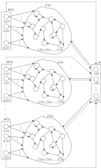
For signals with different time scales, multiple subreser-voirs can build different structures to deal with them. Struc-ture of the multi-reservoirs echo state network is shown in Fig.1.
For D inputs, at time t + 1, state equation and output equation of the model can be denoted by
x1(t + 1) = f1(W1in·u1(t + 1) + W1x·x1(t) +W1back·y(t)) x2(t + 1) = f2(W2in·u2(t + 1) + W2x·x2(t) +W2back·y(t)) ... xD(t + 1) = fD(WDin·uD(t + 1) + WDx ·xD(t)+ WDback·y(t))
y(t + 1) = g(W1out·[(u1(t + 1), x1(t + 1)] + W2out ·[(u2(t + 1), x2(t + 1)] + · · · + WDout
·[(uD(t + 1), xD(t + 1)])
(8)
where [x1(t + 1), x2(t + 1), · · · , xD(t + 1)] and [u1(t + 1), u2(t + 1), · · · , uD(t + 1)] respectively denote D internal units and input units at time t + 1; {W1in, W1x, W1back, W1out}, {W2in, W2x, W2back, W2out}, · · · , {WD
in, WDx, WDback, WDout} are
Dgroups connection weights matrix. {W1in, W1x, W1back, W2in,
W2x, W2back, · · · , WinD, WDx, WDback}is randomly generated in the initialization phase, and {W1out, W2out, · · · , WDout}needs to be trained by input and output of the model.
For the multi-reservoirs echo state network, output of the model can be denoted by following linear equation:
g−1(y(t)) = W1out·[x1(t), u1(t)]T +W2out·[x2(t), u2(t)]T + · · · +WDout·[xD(t), uD(t)]T
=[W1out, W2out, · · · , WDout] · q1(t) q2(t) ... qD(t) (9) where q1(t) = [x1(t), u1(t)]T, q2(t) = [x2(t), u2(t)]T, · · · , qD(t) = [xD(t), uD(t)]T.
FIGURE 1. Structure of the multi-reservoirs ESN model.
For T time steps, the output weight matrix Wout =
[W1out, W2out, · · · , WDout] can be calculated by
Wout=(Q−1·Y )T (10)
where Q = [[q1(1), q2(1), · · · , qD(1)]T, [q1(2), q2(2), · · · ,
qD(2)]T, · · · , [q1(T ), q2(T ), · · · , qD(T )]T]T.
For the multi-reservoirs echo state network model, its predictive performance would be influenced by a total of
D groups {SR, N, IS, SD}. So, IFOA is used to make an optimized selection of them, which will be discussed in Section 5.
IV. PHASE SPACE RECONSTRUCTION (PSR)
In the original data sequence, values of a variable at dif-ferent times are used to reconstruct the phase space, which makes the change of this variable over time can reflect the evolution of the system. Define the original data sequence as: s(1), s(2), · · · , s(n), then time series form by PSR can be
obtained as follows: S1=[s(1), s(1 + γ ), · · · , s(1 + (m − 1)γ )] S2=[s(2), s(2 + γ ), · · · , s(2 + (m − 1)γ )] ... St =[s(t), s(t + γ ), · · · , s(t + (m − 1)γ )] (11)
where m andγ respectively are the embedded dimension and the delay time; t = n − (m − 1)γ , denotes the number of
m-dimension phase points got by n points in the time series. Predicted output of the time series can be expressed by
O(t) = [st+l, st+l+γ, · · · , st+l+(m−1)γ], where l = 1, 2, . . .
means prediction steps. S(t) and O(t) are respectively used as input and output of the model to complete the training and the testing. In the PSR, reasonable m and γ can make the reconstructed system close to the original system. IFOA is used to make an optimized selection of them, which will be discussed in Section 5.
V. VMD-IFOA-ESN MODEL
A. BASIC STRUCTURE
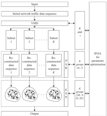
The proposed VMD-IFOA-ESN model uses an integrated optimization strategy by a combination of VMD, PSR, ESN with multi-reservoirs and IFOA, whose basic structure is shown in Fig.2. First, VMD is used to decompose the input network traffic data sequence into K subsets, recorded by
K modes; then for each subset, PSR is used to get the data sequence in high dimensional space; finally, K groups data sequence after PSR are used to train and test the ESN with multi-reservoirs. During the whole prediction, the proposed IFOA method is used to make an optimized selection of several model parameters, include: K andτ in the VMD, m andγ in the PSR and, SR, N, IS and SD in the ESN with multi-reservoirs.
B. IFOA
1) DESCRIPTION OF THE ALGORITHM
IFOA is an improvement of the CMFOA [29], which is combined with the levy’s flight function [30] and cloud model to search the optimal solution. Its main steps are as follows:
Step 1: Generate random initial fruit fly population by
Xi= Vl+(Vh− Vl) · rand () (12)
where [Vl, Vh] is the range of values; rand() is a random value
in [0,1].
Step 2: Find the best individual X _axis in the initial popu-lation, as follows:
Smelli = fitness(Ri) (13)
[bestsmell, bestindex] = min / max(Smell) (14)
smellbest = bestsmell (15)
X_axis = X (bestindex) (16) where fitness(·) denotes fitness function; min/ max(·) denotes minimum/maximum function; bestsmell denotes the
FIGURE 2. Basic structure of the VMD-IFOA-ESN model.
best fitness function value; bestindex denotes the index of the best individual.
Step 3: New individuals are generated by
Xij=
(
Cx(X _axis, En, He), j = d
X_axisj otherwise
(17) where d is a random integer in [1, Z ], Z is the number of decision variables; En and He respectively are entropy and hyperentropy of the cloud generator, calculated by
En = δ · (1 − p maxgen)
α· ϕ · u
(v)1/β (18)
He =0.1 × En (19)
Cx(X _axis, En, He) = exp(−(x − X _axis)
2
2(En0)2 ) (20)
whereδ ∈ (0, 0.5) is iterative adjustment coefficient; α is a positive integer, which is used to define the search accuracy about iterations; p is the number of current iteration, and
maxgenis the maximum number of iterations; u and v satisfy the standard normal distribution, both of which are taken values in the range [0,1]; β ∈ [1, 3]; x ∼ N(Xaxis, En0)
and En0 ∼ N(En, He) satisfy the normal distribution; ϕ is calculated by ϕ = [0(1 + β) · sin(π ·β2) 0(1+β 2 ·β · 2 β−1 2 ) ]β1 (21)
where0(·) is gamma function.
Step 4: For new fruit fly individuals, equations (13) and (14) are used for calculation; if the condition
bestsmell < smellbest is satisfied, equations (15) and (16) are used to update the best solution.
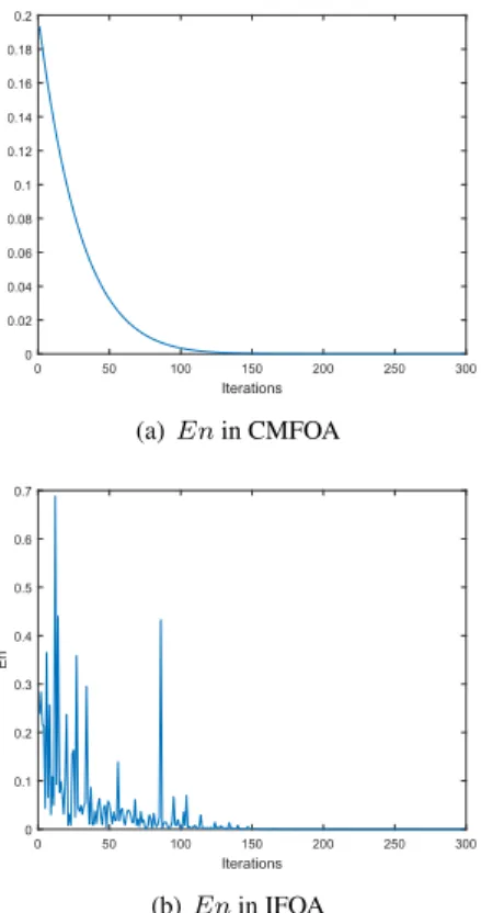
FIGURE 3. Comparison of En in CMFOA and IFOA.
Step 5: Steps 2-4 are repeatedly executed and terminated if the maximum number of iterations reaches; then, output the best solution.
Encan be used as the search radius of fruit fly individuals. Comparisons of changes of En during the whole iterations are shown in Fig.3, whereα = 8, β = 1.5, δ = 0.2, maxgen = 300, and 100 random X _axis in [0, 1] are used as decision variables. As shown in Fig.3(a), the search radius in CMFOA decreases exponentially with increasing number of iterations, which has lager search ranges in the early stage of iterations to find the optimal solution and smaller search radius in the late stage to approach the optimal solution. From Fig.3(b), it can be seen that the search radius in IFOA is overall decreasing with increasing number of iterations; but, some fluctuations can make the search easily jump out of local optimum. Although En in the IFOA decreases gradually in the whole iterations which is the same with En in the CMFOA, En in the IFOA has some sudden changes (with various larger val-ues at different iterations) for the global searching to prevent falling into the local optimum.
2) SIMULATION EXPERIMENT
In order to verify that the proposed IFOA method is advanced, it is compared with other three methods of FOA [24], CMFOA [29] and BCMFOA [31]. Mackey-Glass chaotic series is used for simulation experiment, which is described by
dx(t)
dt =
0.2x(t − η)
η −0.1x(t) (22)
FIGURE 4. Three different network traffic data sequences with different time intervals.
Setη = 30 and x(t) |t=0 = 0.8 to generate 1000 groups
data; random 400 groups for training, and random 200 groups in the rest 600 groups for testing.
TABLE 1. Comparisons of several improved FOA methods.
TABLE 2. Statistical information of three data sequences with different time intervals.
400 groups training samples are used to train IFOA-ESN, FOA-ESN, CMFOA-ESN and BCMFOA-ESN, and 200 groups testing samples are used for testing. Each model is repeatedly executed by 20 times and evaluated by two performance indexes of root mean square error (RMSE) and mean absolute error (MAE), as shown in Table1.
It can be seen from Table 1, compared with three other methods of FOA, CMFOA and BCMFOA, IFOA has better optimal performance for ESN model.
C. ALGORITHM IMPLEMENTATION
The proposed VMD-IFOA-ESN model mainly contains three parts: first, VMD is used to decompose the original network traffic sequence into K subsets (K modes); then, each subset is reconstructed by PSR; finally, K groups reconstructed data sequences are used as input and output of ESN with
K-subreservoirs. Its main steps are as follows:
Step 1: Initialization. Set the maximum number of iter-ations, population size, and the range of the optimized parameters.
Step 2: Initial value of K is randomly given; 6K + 1 fruit fly populations are generated and respectively assigned to τ, mk, γk, SRk, Nk, ISk and SDk, k = 1, 2, · · · , K.
Step 3: Both K andτ are substituted into VMD to decom-pose the original network traffic data sequence into K subsets; for the kth subset, mk andγk are used for the phase space reconstruction; then, SRk, Nk, ISk and SDk are substituted into the kth subreservoir of the multi-reservoirs ESN model using kth reconstructed data sequence for calculation. Posi-tions of the optimal individual in the current 6K + 1 fruit fly populations are determined according to equations (13) - (15) whose values are recorded as the optimal solutions.
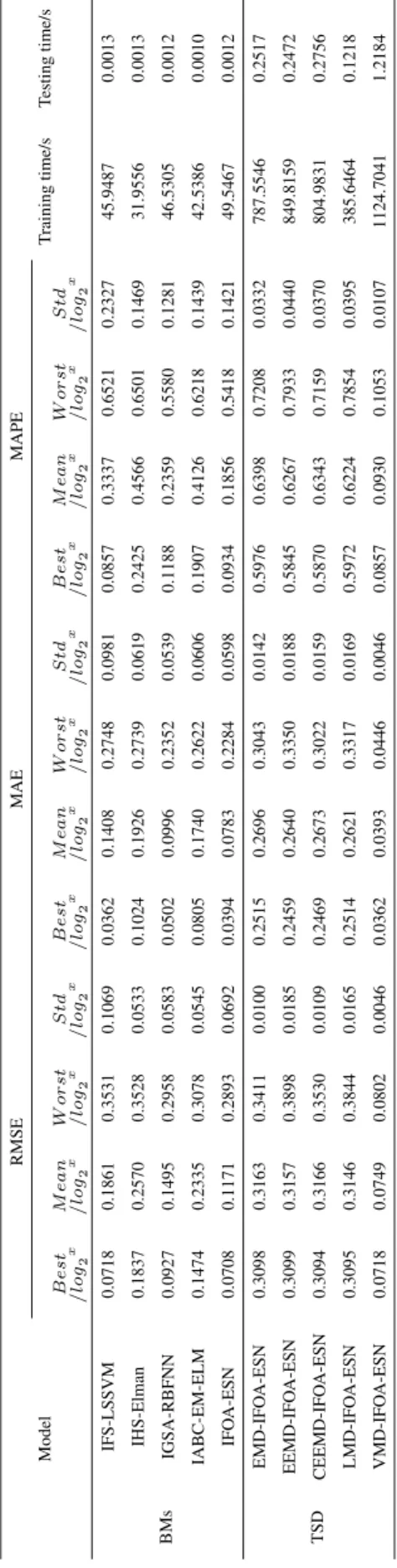
TABLE 3.Predictive performance comparison for ‘‘Day’’ data set by different models.
FIGURE 5. Comparisons of the predicted results by BMs and TSD models for ‘‘Day’’ data set.
Step 4: Positions of each individuals in the 6K + 1 popu-lations are updated according to equations (17) - (21).
Step 5: Equations (13) - (14) are used to calculate posi-tions of new fruit fly individuals; if bestsmell < smellbest is satisfied, the optimal solution is updated according to equations (15) - (16).
Step 6: Steps 2-5 are repeatedly executed until the maxi-mum number of iterations.
Step 7: The best parameters K, τ, mk, γk, SRk, Nk, ISk and SDk are output, and then respectively substituted into VMD, PSR and multi-reservoirs ESN to get the optimal prediction model.
Three performance indexes of RMSE, MAE and mean absolute percentage error (MAPE) are used to evaluate model predictive performance, which are respectively defined by
RMSE = v u u u t Ndata P i=1 (yi− y0i)2 Ndata (23) MAE = 1 Ndata Ndata X i=1 yi− y0i (24) MAPE = 1 Ndata Ndata X i=1 yi− y0i yi ×100% (25)
where Ndata is number of samples; yi and y0i respectively
are the actual value and the predicted value of the ith sample. Because RMSE, MAE and MAPE all reflect the deviation between the actual value and the predicted value, so smaller index value of them stands for better model predic-tive performance. RMSE index is used as fitness function in equation (13).
VI. SIMULATION EXPERIMENTS
WIDE backbone network traffic data by MAWI Working Group are used for simulation experiments. Three data sequences with different time intervals of ‘‘Day’’, ‘‘Hour’’ and ‘‘Minute’’ are selected, which are shown in Table 2.
FIGURE 6. Comparisons of the predicted results by BMs and TSD models for ‘‘Hour’’ data set.
There are 366 groups of data in the ‘‘Day’’ data sequence sampled from 23 July in year 2017 to July 23 in year 2018, whose sampling period is one day; there are 480 groups of data in the ‘‘Hour’’ data sequence sampled from 1 July in year 2018 to July 21 in year 2018, whose sampling period is one hour; and there are 600 groups of data in the ‘‘Minute’’ data sequence sampled from 24 July in year 2018 to July 26 in year 2018, whose sampling period is five minutes.
It can be seen from Table2, samples in three data sequences are recorded by ‘‘byte’’, larger value of which will increase the complexity of data processing. So, in order to reduce the memory capacity and computational complexity, all sam-ples in the original data sequence are taken log of them (log2x, x stands for the sample) [32]. Relative relation of the data will not change after taken the logarithm of them, because the logarithmic function log2xis a monotone increas-ing function in its domain. For three data sets, the original data sequences and the logarithmic function log2x of them are shown in Fig.4.
Comparisons of the predictive performance are car-ried out among the proposed VMD-IFOA-ESN and IFS-LSSVM [1], IHS-Elman [2], IGSA-RBFNN [5], IABC-EM-ELM [4], IFOA-ESN, EMD-IFOA-ESN, EEMD-IFOA-ESN, CEEMD-IFOA-ESN and LMD-IFOA-ESN. IFS-LSSVM, IHS-Elman, IGSA-RBFNN, IABC-EM-ELM and IFOA-ESN belong to basic models (BMs); EMD-IFOA-ESN, EEMD-IFOA-ESN, CEEMD-IFOA-ESN, LMD-IFOA-ESN and VMD-IFOA-ESN belong to TSD models. Some parame-ters are set as follows. Population size is 30 and the maximum number of iterations is 100; in the IFS algorithm, initial value of the search radius is 1, sensitive coefficient of the search radius is 0.9, and step size in the search is 20; in the IHS algorithm, the number of harmonies in the harmony memory library is 6, the maximum and minimum reservation probabilities respectively are 1 and 0.4, the maximum and minimum memory disturbance probabilities respectively are 0.4 and 0.9, the maximum and minimum bandwidth respec-tively are 1 and 0.0001, and the crossed factor is 0.8; in the
FIGURE 7. Comparisons of the predicted results by BMs and TSD models for ‘‘Minute’’ data set.
IGSA algorithm, initial gravity coefficient is 100, iterative coefficient is 20, gravity constant is 2.5, and an arbitrar-ily small positive real number eps; in the IABC algorithm, range of the random step size is [-1,1], range of the posi-tion updating coefficient moving to the optimal soluposi-tion is [0,1], and scaling factor and exponential factor in the adaptive iterative calculation respectively are 50 and 5; in the FOA algorithm, iterative adjustment coefficient δ = 0.2, and two exponential factors in the adaptive iter-ative calculation respectively are α = 2 and β = 2. Several parameter ranges of the multi-subreservoirs model in EMD-IFOA-ESN, EEMD-IFOA-ESN, CEEMD-IFOA-ESN, LMD-IFOA-ESN and VMD-IFOA-ESN are as fol-lows: N ∈ [10, 600], IS ∈ [0.001, 1], SD ∈ [0, 1], SR ∈ [0.0001, 0.1], m ∈ [1, Ndata/15], γ ∈ [1, Ndata/30], K ∈
[1, 20], τ ∈ [0, 4].
The front 316 groups of data in the ‘‘Day’’ data set are used as training samples to train the model and the last 50 groups of data are used as testing samples; in the ‘‘Hour’’ data set, the front 430 groups of data are used as training samples and
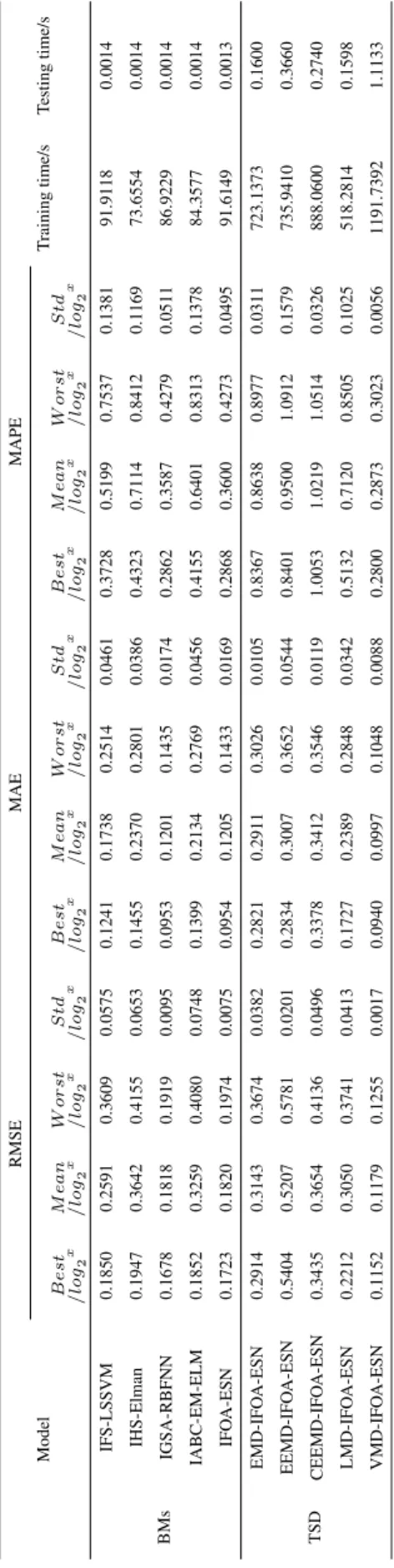
the last 50 groups of data are used as testing samples; and in the ‘‘Minute’’ data set, the front 550 groups of data are used as training samples and the last 50 groups of data are used as testing samples. Computer configurations are as follows: Windows 7 operating system, Intel core i7 4.00GHz CPU, 16GB RAM, Matlab2015a. Each model is repeatedly run for 30 times, and the value of best, mean, worst, std and, average training time and testing time (single running time) under three performance indexes of RMSE, MAE and MAPE are shown in Table3-Table5.
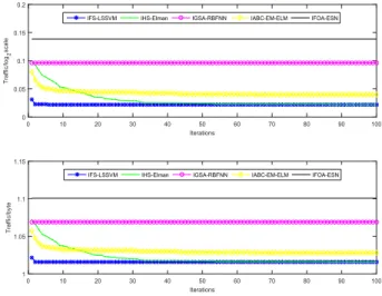
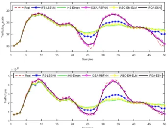
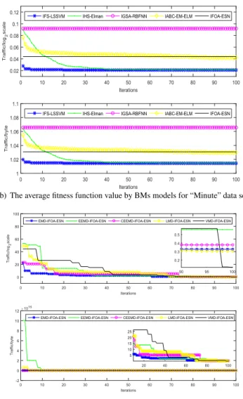
As shown from Table3to Table5, although BMs models have better training speed and calculation performance, they have some deficiencies of unstable optimization results and larger fluctuation of the prediction results; TSD models use signal decomposition method to ensure the stability of the optimization results. Comparisons of the average predicted output value and the average fitness function value by BMs and TMD models are shown from Fig.5. to Fig.7.
From Figs.5-7, for three network traffic data sets with different time interval, TSD models have better predictive
TABLE 4. Predictive performance comparison for ‘‘Hour’’ data set by different models.
TABLE 5.Predictive performance comparison for ‘‘Minute’’ data set by different models.
FIGURE 8. Change curves of the optimal average N for three data sets by TSD models.
stability than BMs models. Multiple subreservoirs with dif-ferent structure parameters are trained by TSD models which can reduce negative influences for the model predictive per-formance produced by different changing laws of the data. During the training phase, comparisons of the optimal
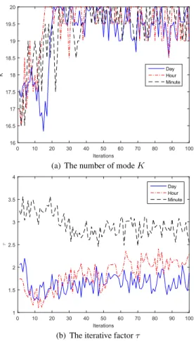
aver-FIGURE 9. Change curves of K andτ in VMD-IFOA-ESN model for three data sets during the training phase.
age reservoir scale (N ) of four models of EMD-IFOA-ESN, EEMD-IFOA-ESN, CEEMD-IFOA-ESN and LMD-IFOA-ESN are shown in Fig.8.
It can be seen from Fig.8, during the training phase, the number of reservoirs have no changes which makes that the model predictive performance is improved only by optimization of internal structure of these reservoirs. Different with four models of EMD-IFOA-ESN, EEMD-IFOA-ESN, CEEMD-IFOA-ESN and LMD-EEMD-IFOA-ESN, VMD-IFOA-ESN uses a strategy of inside and outside opti-mization of the reservoir, of which the number of reservoirs are optimized and all structure parameters of each subreser-voirs are optimized at the same time. Changes of the optimal average value of the number of modes K and the iterative factorτ in the VMD-IFOA-ESN model are shown in Fig.9.
As shown in Fig.9, during the training phase, dynamic changes of the number of mode K will make the number of subreservoirs have same adjustment along with it. The inside and outside optimization of the reservoir will improve the model predictive performance, because this dynamic adjust-ment mechanism could make the prediction model be less affected by the nonlinear and nonstationary data set.
VII. CONCLUSION
In order to reduce bad effects caused by nonlinear and non-stationary of the data sequence in the network traffic
predic-tion, a prediction model based on signal decomposition and multi-reservoirs echo state network is proposed in this paper. VMD is used to decompose the original data set into several subsets which are then reconstructed by PSR. Then, an ESN model with multiple subreservoirs is built according to the number of subreservoirs whose outputs are integrated for the final output. An improved FOA algorithm is proposed for parameter optimization in VMD, PSR and multi-reservoirs ESN. Main conclusions of our works are summarized as follows:
(1) For the nonlinear and nonstationary of the actual network traffic data, the multi-reservoirs structure could effectively deal with the problem of different structural parameters of phase space reconstruction. In this paper, the multi-reservoirs structure was built and multiple subreser-voirs were trained to adapt to different data changing laws, which could increase stability of the prediction for nonlinear and nonstationary time series. From Tables3-5, compared with BMs models, the signal decomposition based multi-reservoirs ESN model had better prediction stability. More-over, as shown in Fig.5(c)-(d), Fig.6(c)-(d) and Fig.7(c)-(d), compared with the other TSD models, the proposed VMD-IFOA-ESN model had better convergence performance and prediction precision.
(2) VMD was used to transform the signal decomposition problem into a constrained optimization problem. Compared with EMD, EEMD, CEEMD and LMD, it had some advan-tages of avoiding the mode aliasing, decreasing endpoint effects, and robustness of noise interference. In the proposed VMD-IFOA-ESN, IFOA algorithm was used to optimally select the best K and τ according to the training samples, which made the signal decomposition be independent of the prior knowledge. As shown in Fig.8 and Fig.9, during the training phase, K remained the same in four methods of EMD, EEMD, CEEMD and LMD, but K was dynamically optimized by training performance of the model. This opti-mization based signal decomposition strategy could increase adaptability of the prediction model to the signal with noise and nonlinearity.
(3) An improved FOA algorithm (IFOA) based on the cloud model was proposed, which combined the levy’s flight function and cloud generator to generate new fruit fly indi-viduals. As shown in Fig.3, the search radius was overall decreasing along with iterations and had some fluctuations during searching process. These random fluctuations for the search radius had advantages of increasing population diver-sity and easily jumping out of the local optimum. Seen from Table1, IFOA had better prediction performance than some other improved IFOA algorithms.
However, as shown from Tables3-5, compared with other TSD models, the VMD-IFOA-ESN model needed longer calculation time, which was due to synchronous optimization inside and outside of the multiple subreservoirs. Therefore, in our future works, we aim to search on how to reduce the calculation time on the basis of ensuring the prediction performance.
REFERENCES
[1] Z. Tian and S. Li, ‘‘A network traffic prediction method based on IFS algorithm optimised LSSVM,’’ J. Eng. Syst. Model. Simul., vol. 19, no. 4, pp. 200–213, 2017.
[2] Z. Tian, S. Li, Y. Wang, and X. Wang, ‘‘A network traffic hybrid prediction model optimized by improved harmony search algorithm,’’ Neural Netw. world, vol. 25, no. 6, pp. 669–686, 2015.
[3] V. Alarcon-Aquino and J. A. Barria, ‘‘Multiresolution FIR neural-network-based learning algorithm applied to network traffic prediction,’’ IEEE Trans. Syst., Man, Cybern., C (Appl. Rev.), vol. 36, no. 2, pp. 208–220, Mar. 2006.
[4] Z. Tian, S. Li, Y. Wang, and X. Wang, ‘‘Network traffic prediction method based on improved ABC algorithm optimized EM-ELM,’’ J. China Uni-versities Posts Telecommun., vol. 25, no. 3, pp. 33–44, 2018.
[5] D. Wei, ‘‘Network traffic prediction based on RBF neural network opti-mized by improved gravitation search algorithm,’’ Neural Comput. Appl., vol. 28, no. 8, pp. 2303–2312, 2017.
[6] Z. Tian and T. Shi, ‘‘Time-delay prediction method based on improved genetic algorithm optimized echo state networks,’’ in Proc. Chin. Intell. Syst. Conf., 2016, pp. 209–220.
[7] G. Shi, D. Liu, and Q. Wei, ‘‘Energy consumption prediction of office buildings based on echo state networks,’’ Neurocomputing, vol. 216, pp. 478–488, 2016.
[8] L. Zhang, C. Hua, Y. Tang, and X. Guan, ‘‘Ill-posed echo state network based on l-curve method for prediction of blast furnace gas flow,’’ Neural Process. Lett., vol. 43, no. 1, pp. 97–113, 2016.
[9] S. Zhong, X. Xie, L. Lin, and F. Wang, ‘‘Genetic algorithm optimized double-reservoir echo state network for multi-regime time series predic-tion,’’ Neurocomputing, vol. 238, pp. 191–204, May 2017.
[10] L. Wang, H. Hu, X.-Y. Ai, and H. Liu, ‘‘Effective electricity energy consumption forecasting using echo state network improved by differential evolution algorithm,’’ Energy, vol. 153, pp. 801–815, Jun. 2018. [11] M. Han and D. Mu, ‘‘Multi-reservoir echo state network with sparse
Bayesian learning,’’ in Proc. Int. Symp. Neural Netw., 2010, pp. 450–456. [12] M. J. A. Rabin, M. S. Hossain, M. S. Ahsan, M. A. S. Mollah, and M. T. Rahman, ‘‘Sensitivity learning oriented nonmonotonic multi reser-voir echo state network for short-term load forecasting,’’ in Proc. Int. Conf. Inform., Electron. Vis. (ICIEV), 2013, pp. 1–6.
[13] Z. Lv, J. Zhao, Y. Liu, and W. Wang, ‘‘Use of a quantile regression based echo state network ensemble for construction of prediction intervals of gas flow in a blast furnace,’’ Control Eng. Pract., vol. 46, pp. 94–104, Jan. 2016.
[14] J. Qiao, F. Li, H. Han, and W. Li, ‘‘Growing echo-state network with multiple subreservoirs,’’ IEEE Trans. Neural Netw. Learn. Syst., vol. 28, no. 2, pp. 391–404, Feb. 2016.
[15] C. Li, Z. Xiao, X. Xia, W. Zou, and C. Zhang, ‘‘A hybrid model based on synchronous optimisation for multi-step short-term wind speed forecast-ing,’’ Appl. Energy, vol. 215, pp. 131–144, Apr. 2018.
[16] Z. Tian, S. Li, Y. Wang, and S. Yi, ‘‘A prediction method based on wavelet transform and multiple models fusion for chaotic time series,’’ Chaos, Solitons Fractals, vol. 98, pp. 158–172, May 2017.
[17] N. E. Huang, Z. Shen, S. R. Long, M. C. Wu, H. H. Shih, Q. Zheng, N.-C. Yen, C. C. Tung, and H. H. Liu, ‘‘The empirical mode decomposition and the Hilbert spectrum for nonlinear and non-stationary time series analysis,’’ Proc. Roy. Soc. London Ser. A, Math., Phys. Eng. Sci., vol. 454, no. 1971, pp. 903–995, Mar. 1998.
[18] Z. Wu and N. E. Huang, ‘‘Ensemble empirical mode decomposition: A noise-assisted data analysis method,’’ Adv. Adapt. Data Anal., vol. 1, no. 1, pp. 1–41, 2008.
[19] J. R. Yeh, J. S. Shieh, and N. E. Huang, ‘‘Complementary ensemble empirical mode decomposition: A novel noise enhanced data analysis method,’’ Adv. Adapt. Data Anal., vol. 2, no. 2, pp. 135–156, 2010. [20] J. S. Smith, ‘‘The local mean decomposition and its application to EEG
perception data,’’ J. Roy. Soc. Interface, vol. 2, no. 5, pp. 443–454, 2005. [21] K. Dragomiretskiy and D. Zosso, ‘‘Variational mode decomposition,’’
IEEE Trans. Signal Process., vol. 62, no. 3, pp. 531–544, Feb. 2014. [22] D. Wang, H. Guo, H. Luo, O. Grunder, and Y. Lin, ‘‘Multi-step ahead
electricity price forecasting using a hybrid model based on two-layer decomposition technique and BP neural network optimized by firefly algorithm,’’ Appl. Energy, vol. 190, pp. 390–407, Mar. 2017.
[23] M. Niu, Y. Hu, S. Sun, and Y. Liu, ‘‘A novel hybrid decomposition-ensemble model based on VMD and HGWO for container throughput forecasting,’’ Appl. Math. Model., vol. 57, pp. 163–178, May 2018.
[24] W.-T. Pan, ‘‘A new fruit fly optimization algorithm: Taking the financial distress model as an example,’’ Knowl.-Based Syst., vol. 26, pp. 69–74, Feb. 2012.
[25] W. Wang and X. Liu, ‘‘Melt index prediction by least squares support vec-tor machines with an adaptive mutation fruit fly optimization algorithm,’’ Chemometrics Intell. Lab. Syst., vol. 141, pp. 79–87, Feb. 2015. [26] X. Yuan, Y. Liu, Y. Xiang, and X. Yan, ‘‘Parameter identification of BIPT
system using chaotic-enhanced fruit fly optimization algorithm,’’ Appl. Math. Comput., vol. 268, pp. 1267–1281, Oct. 2015.
[27] M.-W. Li, J. Geng, D.-F. Han, and T.-J. Zheng, ‘‘Ship motion predic-tion using dynamic seasonal RvSVR with phase space reconstrucpredic-tion and the chaos adaptive efficient FOA,’’ Neurocomputing, vol. 174, no. 4, pp. 661–680, 2016.
[28] S. Kanarachos, J. Griffin, and M. E. Fitzpatrick, ‘‘Efficient truss optimiza-tion using the contrast-based fruit fly optimizaoptimiza-tion algorithm,’’ Comput. Struct., vol. 182, no. 1, pp. 137–148, 2017.
[29] L. Wu, C. Zuo, and H. Zhang, ‘‘A cloud model based fruit fly optimization algorithm,’’ Knowl.-Based Syst., vol. 89, pp. 603–617, Nov. 2015. [30] B. Yan, Z. Zhao, Y. Zhou, W. Yuan, J. Li, J. Wu, and D. Cheng, ‘‘A
par-ticle swarm optimization algorithm with random learning mechanism and levy flight for optimization of atomic clusters,’’ Comput. Phys. Commun., vol. 219, pp. 79–86, Oct. 2017.
[31] L. Wu, C. Zuo, H. Zhang, and Z. Liu, ‘‘Bimodal fruit fly optimization algorithm based on cloud model learning,’’ Soft Comput., vol. 21, no. 7, pp. 1877–1893, 2017.
[32] R. Fontugne, P. Abry, K. Fukuda, D. Veitch, K. Cho, P. Borgnat, and H. Wendt, ‘‘Scaling in Internet traffic: A 14 year and 3 day longitudi-nal study, with multiscale alongitudi-nalyses and random projections,’’ IEEE/ACM Trans. Netw., vol. 25, no. 4, pp. 2152–2165, Aug. 2017.
YING HAN received the B.Sc. and M.Sc. degrees from Liaoning Technical University, Fuxin, China, in 2005 and 2008, respectively. She is currently pursuing the Ph.D. degree with Northeastern Uni-versity, Shenyang, China. She is currently with the College of Engineering, Bohai University, Jinzhou, China. Her research interests include time series analysis and application and complex system prediction.
YUANWEI JING received the B.S. degree in mathematics from Liaoning University, Liaoning, China, in 1981, and the M.S. and Ph.D. degrees in automatic control from Northeastern University, Shenyang, China, in 1984 and 1988, respectively. From 1998 to 1999, he was a Senior Visiting Scholar with Computer Science Telecommunica-tion Program, University Missouri–Kansas City. He is currently with the School of Information Science and Engineering, Northeastern University. His current research interests include control problems in modern communi-cation network systems, networks traffic management, analysis and control, control of flight craft, and analysis and control of large-scale complex nonlinear systems.
KUN LI received the B.Sc. degree from the Shandong University of Science and Technology, in 2005, the M.Sc. degree from Liaoning Tech-nical University, in 2008, and the Ph.D. degree from Northeastern University, Shenyang, China, in 2013. He is currently an Associate Professor with the College of Engineering, Bohai Univer-sity. His current research interests include complex industrial process modeling, intelligent optimal control, machine learning, and their applications. GEORGI MARKO DIMIROVSKI received the B.S. degree in electrical engineering from the Saints Cyril and Methodius University of Skopje, Macedonia, in 1966, the M.S. degree in electrical and electronic engineering from the University of Belgrade, Serbia, in 1974, and the Ph.D. degree in automatic control from the University of Bradford, Bradford, England, in 1977. He is currently a Pro-fessor with the School of Engineering Department, Dogus University, Istanbul, Turkey, and the School FEIT, Saints Cyril and Methodius University of Skopje, Skopje, Macedonia. He has contributed the followings: one research monograph with Springer international, 17 chapters in research monographs, and more than 100 journal articles as well as more than 360 articles in the IEEE and IFAC proceed-ings series alone. His current research interests include complex dynamic networks and systems, fuzzy-logic and neural-network topics of applied computational intelligence, and switched systems and switching control.