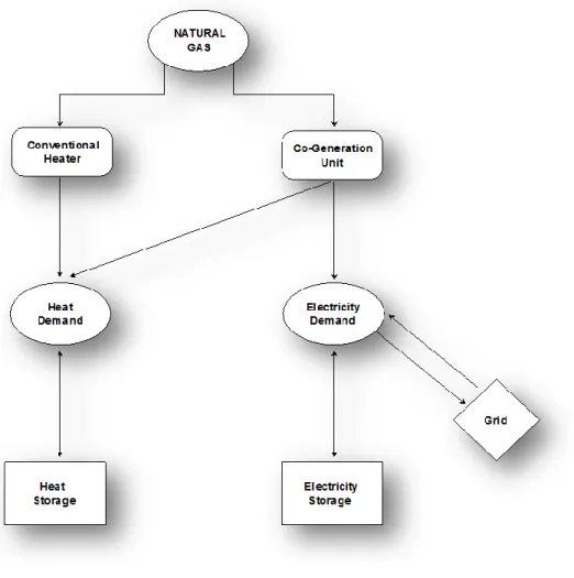
Model for valuating decentralized energy production

As with each time series analysis, before modeling volatility in natural gas prices series, the stationarity analysis will be studied using ACFs and unit root

Tender offer: The hunter compa- ny makes an offer to the shareholders of the target company for the takeover of their shares at the current market (stock market ) price.. Th offer

The turning range of the indicator to be selected must include the vertical region of the titration curve, not the horizontal region.. Thus, the color change

For this reason, there is a need for science and social science that will reveal the laws of how societies are organized and how minds are shaped.. Societies have gone through

• The first book of the Elements necessarily begin with headings Definitions, Postulates and Common Notions.. In calling the axioms Common Notions Euclid followed the lead of

With the gas disruptions to the European Union in 2006 and 2009 Ukrainian crises, the Community decided to diversify its supply sources and routes, develop energy

Since regional stability in the Eastern Mediterranean cannot be achieved with the natural gas reserves in the Aphrodite field, the ethnic conflict between the Turkish and the

In order to ensure supply security, the SEE countries try to diversify their suppliers and supply routes, increase their domestic production and decrease the consumption of