a thesis
submitted to the department of computer engineering
and the institute of engineering and science
of bilkent university
in partial fulfillment of the requirements
for the degree of
master of science
By
Ta˘
gma¸c Topal
January, 2004
Assist. Prof. Dr. ˙Ibrahim K¨orpeo˘glu(Advisor)
I certify that I have read this thesis and that in my opinion it is fully adequate, in scope and in quality, as a thesis for the degree of Master of Science.
Prof. Dr. Cevdet Aykanat
I certify that I have read this thesis and that in my opinion it is fully adequate, in scope and in quality, as a thesis for the degree of Master of Science.
Prof. Dr. ¨Ozg¨ur Ulusoy
Approved for the Institute of Engineering and Science:
Prof. Dr. Mehmet B. Baray Director of the Institute
SCATTERNETS
Ta˘gma¸c Topal
M.S. in Computer Engineering
Supervisor: Assist. Prof. Dr. ˙Ibrahim K¨orpeo˘glu January, 2004
Among various technologies for short-range wireless networking, Bluetooth has received a particular attention from users as well as from vendors. It is the main technology that supports wireless personal area networking. Bluetooth Special Interest Group (SIG), which is a consortium established to develop and promote the technology, produces the specifications of Bluetooth standards. The Bluetooth standards specify the building blocks to construct Bluetooth networks of arbitrary size, i.e. scatternets, but they do not specify the policies and algo-rithms that can be used in constructing these scatternets. There may be various approaches for forming Bluetooth scatternets which will result in different topolo-gies for the same set of nodes.
In this thesis, we first define and provide some performance metrics that can be used to evaluate various scatternet topologies that can be the output of different scatternet formation algorithms. Then, we provide a new Bluetooth scatternet construction algorithm that differs from other algorithms in that it also considers the traffic pattern of users (i.e. traffic requirements of nodes among themselves) in establishing a scatternet. Then we evaluate the performance of our algorithm through simulations by observing the properties of the constructed scatternets. In a scatternet that is the result of our algorithm we particularly look to the weighted average shortest path lengths that traffic flows follow, the ratio of satisfied users, and the utilization of the scatternet capacity. The results show that we can achieve a good ratio of satisfied users, a high network utilization, and a reasonably small value for average path lengths using our algorithm. The algorithm is currently centralized, but can be extended to a distributed one in the future.
Keywords: Bluetooth, Scatternet Construction, Efficient Topologies, Wireless Personal Area Networks, Traffic Requirements.
Ta˘gma¸c Topal
Bilgisayar M¨uhendisli˘gi, Y¨uksek Lisans Tez Y¨oneticisi: Yrd. Do¸c. Dr. ˙Ibrahim K¨orpeo˘glu
Ocak, 2004
C¸ e¸sitli kısa mesafeli kablosuz a˘g teknolojileri arasında, Bluetooth hem kul-lanıcılardan hem de ¨ureticilerden belirgin bir ilgi g¨or¨uyor. Bluetooth, kablo-suz ki¸sisel alan a˘gları destekleyen ana teknoloji durumunda. Teknolojiyi geli¸stirmek ve tanıtmak amacıyla kurulan Bluetooth Special Interest Group (SIG), Bluetooth standartlarının belirtimlerini ¨uretmekte. Bluetooth standart-ları, de˘gi¸sen boyutlarda Bluetooth a˘gları, serpme a˘glar (scatternet), olu¸sturmak i¸cin gerekli yapı ta¸slarını belirtiyor ama bu serpme a˘gların olu¸sturulmasında kul-lanılabilecek politika ve algoritmaları belirtmiyor. Bluetooth serpme a˘glarının bi¸cimlendirilmesinde, aynı d¨u˘g¨um k¨umesinden farklı ilingelerin elde edilmesini sa˘glayacak de˘gi¸sik yakla¸sımlar olabilir.
Tez ¸calı¸smamızda, ilk olarak farklı serpme a˘g bi¸cimlendirme algoritmalarının ¸cıktısı olan serpme a˘g ilingelerini de˘gerlendirmek i¸cin bazı ba¸sarım metrikleri tanımladık. Daha sonra, serpme a˘g kurulmasında kullanıcı trafik desenlerini (d¨u˘g¨umlerin birbirleri arasındaki bilgi trafi˘gi gereksinimleri) dikkate almasıyla di˘ger algoritmalardan ayrılan yeni bir Bluetooth serpme a˘g olu¸sturma algorit-ması geli¸stirdik. Ardından, benzetimlerle, olu¸sturulan serpe a˘gların ¨ozelliklerini g¨ozlemleyerek algoritmamızın ba¸sarımını inceledik. Algoritmamızın ¨ur¨un¨u olan bir serpme a˘gda ¨ozellikle, trafik akı¸slarının izledi˘gi en kısa a˘gırlıklı ortalamalı yol uzunluklarına, tatmin edilen kullanıcı oranına ve tahsis edilen trafik kapasitesi oranına baktık. Sonu¸clar bize, algoritmamızı kullanarak y¨uksek oranlarda kul-lanıcı tatminine, y¨uksek oranlarda kapasite tahsisine ve d¨u¸s¨uk de˘gerlerde en kısa a˘gırlıklı ortalamalı yol uznuklarına ula¸sabilece˘gimizi g¨osterdi. S¸u anda, algorit-mamız merkezi yapıda ama gelecekte da˘gıtık yapıya d¨on¨u¸st¨ur¨ulebilir.
Anahtar s¨ozc¨ukler : Bluetooth, Serpme A˘g Olu¸sturma, Verimli ˙Ilingeler, Ki¸sisel Kablosuz ˙Ileti¸sim A˘gları, Trafik Gereksinimleri.
I would like to express my gratitude to my supervisor Assist. Prof. Dr. ˙Ibrahim K¨orpeo˘glu for his great efforts and instructive comments in the supervi-sion of the thesis.
I would like to express my thanks and gratitude to Prof. Dr. Cevdet Aykanat and Prof. Dr. ¨Ozg¨ur Ulusoy for evaluating my thesis.
I should express my thanks to my dear friends for their help in this research; H. ¨Ozg¨ur Tan for his accompany during the research, Berkant B. Cambazo˘glu for his help in developing the simulation environment.
I would like to express my special thanks to my parents for their endless love and support throughout my life. Without them, life would not be that easy and beautiful. . .
1 Introduction 1
1.1 Motivation . . . 2
2 Background and Related Work 7 2.1 Bluetooth Technology . . . 7
2.1.1 Overview . . . 7
2.1.2 Network Topologies . . . 9
2.1.3 Packets . . . 12
2.1.4 Connection Establishment and Piconet Formation . . . 17
2.1.5 Constructing and Operating Scatternets . . . 21
2.2 Related Work . . . 23
3 Scatternet Formation Algorithm 27 3.1 Performance Metrics for Scatternets . . . 27
3.2 Scatternet Formation with Traffic Consideration (FTC) algorithm 31 3.2.1 Overview . . . 31
3.2.2 Traffic information . . . 32
3.2.3 Master selection . . . 33
3.2.4 Bridge selection . . . 35
3.2.5 Maximum path length . . . 36
3.2.6 Data Structures . . . 37
3.2.7 Construction Algorithm . . . 43
3.2.8 Join operation . . . 48
3.2.9 Node share operation . . . 50
3.2.10 Piconet share operation . . . 52
3.2.11 Analysis of the Algorithm . . . 53
4 Simulation and Results 54 4.1 Experiment Environment . . . 54
4.2 Results and Evaluation . . . 55
5 Conclusion and Future Work 60
A Table of Acronyms 65
1.1 Piconet with 6 nodes . . . 3
1.2 Scatternet with 2 piconets . . . 4
1.3 Intra-piconet data traffic in a scatternet . . . 5
1.4 Inter-piconet data traffic in a scatternet . . . 5
2.1 Multi-slot packets . . . 8
2.2 Polling in piconet . . . 10
2.3 Data Packet Content . . . 12
2.4 Connection States . . . 18
3.1 Traffic flow list . . . 38
3.2 Operations in Traffic flow list . . . 39
3.3 Operations in Traffic flow list - 2 . . . 39
3.4 Connectivity matrix . . . 40
3.5 Distance values in a scatternet . . . 41
3.6 Traffic Load . . . 42
3.7 Node list . . . 43
3.8 Piconet list of a scatternet . . . 44
3.9 Initial traffic demand values . . . 45
3.10 Procedures to provide connectivity . . . 46
3.11 Join operation . . . 47
3.12 Node share operation . . . 48
3.13 Piconet share operation . . . 49
4.1 Weighted Shortest Path . . . 56
4.2 Topology Utilization - Block Ratio . . . 57
4.3 Demand per Node - Block Ratio . . . 58
2.1 Operating frequency bands . . . 7
2.2 Link control packets . . . 14
2.3 ACL packets . . . 15
2.4 SCO packets . . . 16
2.5 Inquiry, Inquiry Scan messages . . . 20
2.6 Page, Page Scan messages . . . 20
Introduction
The advances in capabilities of mobile devices increased the use of mobile digital information devices such as mobile computers, cellular phones, and personal dig-ital assistants (PDAs). Importance of networking for this kind of devices using wireless communication technologies increases everyday since the success of these devices on the market lies primarily in their offerings of accessing data anywhere and anytime. Like wired networks, wireless communication technologies can also be categorized into different classes. One criteria for categorization is the range of communication that wireless technologies offer. Mobile devices like PDAs and mobile computers generally require short-range wireless access to reach to dis-tributed data and computation resources and the Internet. Since these devices usually operate with energy-limited batteries, wireless access solution for these devices has to be also efficient in energy consumption, i.e. the wireless technology should be low-power. However, short-range and local area data access and Inter-net access require quite high bit-rates for transmission of data. Therefore, wireless access technologies for these devices should also have high capacity in terms of bandwidth. This kind of short-range, high data-rate, low-power wireless network technologies are classified as Wireless Personal Area Networks (WPAN). There is a working group of IEEE, called IEEE 802.15 [1], that works on the standard-ization of this class of technologies. WPANs should support mobility and also ad-hoc mode of operation. They are characterized by being low-power, low-cost,
and having high data-rate.
In the area of short-range wireless technologies, Bluetooth is a wireless tech-nology that has received a particular attention from users as well as from vendors. It has been initiated by five big computer and communication companies, IBM, Ericsson, Intel, Nokia, and Toshiba. A Bluetooth Special Interest group (SIG) has been formed with the leadership of these companies. The SIG produced the first specification of Bluetooth standards in 1999. Now, Bluetooth standardization ef-forts are continued under the IEEE 802.15 Working Group for Wireless Personal Area Networks. Bluetooth is the main technology in this Working Group that supports wireless personal area networking [2][3][4].
1.1
Motivation
Bluetooth is an RF technology designed for personal area networking. Bluetooth devices generally have a range of 10 meters and they operate in the 2.4 - 2.4835 GHz ISM band. Different from other wireless systems that are using the allocated band as one big channel, Bluetooth divides the allocated band of 84 MHz into 79 RF channels each having 1 MHz bandwidth and 1 Mbps capacity. Bluetooth uses a frequency hopping spread spectrum (FHSS) technique, using which a Blue-tooth device hops through these 79 channels in a rate of 1600 hops per second. Each device follows a pseudo-random hopping sequence. All devices in a small Bluetooth network, called piconet, use the same hopping pattern. Every piconet has its own hopping pattern. This reduces the interference between neighboring piconets. Use of frequency hopping also enables a basic level of security for de-vices that are part of a piconet, because a sniffer that tries to listen to the piconet traffic has to know the frequency hopping pattern of the piconet in order to be able to decode the packets. The hopping sequence of devices in a piconet are determined from the 48 bit Bluetooth address of the master of the piconet.
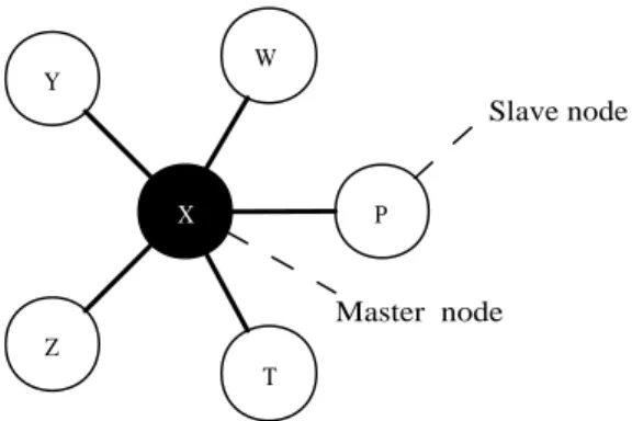
According to the Bluetooth specification, a piconet can have at most eight active members at a given time. A piconet is structured using a start-topology,
where the node in the center is called master, and others are called slaves (see Figure 1.1). This implies that there can be at most one master and seven slaves in a piconet. Y T P W Z X Slave node Master node
Figure 1.1: Piconet with 6 nodes
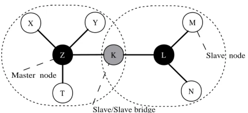
When multiple piconets share a coverage area with intersecting regions, they can establish a bigger Bluetooth network, called scatternet (see Figure 1.2). A scatternet does not have any limit on the number of nodes that it can have provided that the connectivity between piconets can be achieved. In a scatternet, besides data transfers between nodes of the same piconet, there may be data transfers between nodes that belong to different piconets of the same scatternet. In order to connect multiple piconets together some nodes act as members of multiple piconets at the same time and establish the connectivity between these piconets. These special nodes are called bridges. A bridge node can be active only in one piconet at a given time and follows the frequency hopping pattern of that piconet during this time. When the bridge node switches to another piconet to take part in that piconet, it has to follow the frequency hopping pattern of that piconet. By switching between multiple piconets and by use of buffering, a bridge node enables flow of inter-piconet traffic among multiple piconets.
There is a centralized control within a Bluetooth piconet. The master node schedules the traffic in the piconet and determines the frequency to be used. The hopping sequence of the piconet is determined by the master’s Bluetooth address. Master of a piconet also coordinates the access to the shared radio channel that the piconet uses via a polling-based TDMA scheme. The master periodically
X T M Y N Z K L Master node Slave node Slave/Slave bridge
Figure 1.2: Scatternet with 2 piconets
polls the slaves in the piconet. A slave can use the channel only when it is polled by the master. When a slave is polled, it can send data at the next-time slot. A master can also send a data packet directly to a slave instead of just polling the slave. All packets transferred in the piconet have to go over the master, i.e. slaves can not send data to each other directly.
When two nodes in the same piconet communicate, the length of the path that data packets travel is either one or two depending on the role of the nodes in the piconet (master or slave). If one of the nodes is the master of that piconet, then the length of the path is one (see Figure 1.3(b)). If both nodes are slaves, then the length of the path is two: one hop from the slave that is the source of packet to the master, and another hop from the master to the slave that is destination of the packet (see Figure 1.3(a)). This shows that even inside a single piconet the same packet may consume different number of time-slots depending on the roles of its source and destination nodes. Therefore, end-to-end latency and total power consumed during transportation of packets may be different depending on the roles of source and destination.
When there is communication between nodes that belong to different piconets, packets travel longer paths. In Figure 1.4 we see a communication path between two nodes, X and Y, that belong to two different piconets. The piconets are connected with each other through a bridge node, which is node Z in the figure. Every packet sent by X to Y traverses four links (X-M-Z-P-Y) and is received and
X
T
(a) Communication between slave nodes (b) Communication between the master and a slave node W Y Z K M L N
Figure 1.3: Intra-piconet data traffic in a scatternet
forwarded by three intermediate nodes, M, Z, and P. None of these three nodes are either source nor the destination of the traffic. Bluetooth enabled devices are generally mobile devices running on batteries, which means minimizing energy consumption is very important for them. However, as seen in the figure the intermediate nodes, which can be battery-powered mobile devices, are using their energy to forward the traffic that has nothing to do with them.
K X Z T S M Y R Q P
Figure 1.4: Inter-piconet data traffic in a scatternet
Current Bluetooth specification involves a definite description of piconet con-struction with details about the stages of concon-struction and handshaking protocols between devices. For constructing scatternets, however, the specification does not provide any algorithm. It only describes some restrictions on topological struc-tures that limit possible scatternet topologies. According to these restrictions a node can be master only in one piconet but can be slave in multiple piconets.
Formation procedures of scatternets is an open research issue.
There are previous studies in the field of scatternet formation. Many of these proposals focus on time and message complexity of their formation algorithms, and some of them try to construct topologies that are easier to manage and route packets on them. Some other studies that give protocols and algorithms about dynamic formation of scatternets do not consider traffic requirements of users that will use those scatternets, nor the capacity of resulting scatternets. Miklos [5] and Zurbes [6], however, state that the topology of a scatternet has a great influence on its capacity and performance. In an other study by Miorandi [7], it is argued that even the roles taken by the nodes of a piconet affect the performance of the system.
Background and Related Work
2.1
Bluetooth Technology
2.1.1
Overview
Bluetooth is a short-range radio technology that operates in the unlicensed Indus-trial, Scientific and Medical (ISM) band at 2.4 GHz. Bluetooth radio frequency range is usually 10 meters, and it enables portable and mobile devices to com-municate in an ad hoc manner without consuming much battery power. The Bluetooth uses the ISM band, which occupies 2400 - 2483,5 MHz range, but some countries reserved some parts of the ISM band for some other purposes. In these countries smaller fractions of the ISM band can be used by Bluetooth devices. [2] [3] [4]
Geography Regulatory Range RF Channels
USA, Europe and most 2.4000 - 2.4835 GHz f = 2402+k MHz k= 0,. . . ,78 other countries
Table 2.1: Operating frequency bands
As mentioned earlier, the allocated band for Bluetooth is divided into 79 7
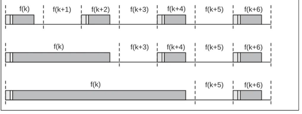
channels each having a MHz channel bandwidth. Bluetooth uses FHSS technique so that each device hops through 79 channels using a pseudo-random hopping sequence that is determined from the Bluetooth address of piconet master. The hopping rate is fast and it is 1600 hops/seconds. The hopping period, which is 625 µs, is also the duration of a time-slot. Bluetooth uses baseband packets that can span 1, 3, or 5 time-slots (see figure 2.1) [2]. The capacity of a frequency hopping channel is 1 Mbps. Each Bluetooth packet is sent at a different frequency. For packets that span multiple time-slots, however, the frequency is not changed until the packet is fully transmitted. Bluetooth uses TDD (Time Division Duplex) scheme is as the duplexing method to provide two-way communication.
f(k) f(k+1) f(k) f(k) f(k+2) f(k+3) f(k+3) f(k+4) f(k+5) f(k+6) f(k+6) f(k+6) f(k+5) f(k+5) f(k+4)
Figure 2.1: Multi-slot packets
Bluetooth protocol can use synchronous or asynchronous connections depend-ing on the application type to carry application traffic. For transmission of data asynchronous connections are used. For transmission of voice, which is a time-critical application, synchronous connections are used. A Bluetooth channel can support up to three simultaneous 64 Kbps synchronous voice connections or a combination of voice and data connections. Maximum data-rate of an asyn-chronous connection is 723.2 Kbps asymmetric (forward and reverse traffic have different data-rates), or 433.9 Kbps symmetric (forward and reverse traffic have the same data-rate).
2.1.2
Network Topologies
In Bluetooth technology, a frequency hopping channel is shared by at most eight active Bluetooth devices communicating with each other. This group of nodes are called piconet in Bluetooth terminology (see Figure 1.1). There may be more than eight members of a piconet but only eight of the members are assigned active member addresses (AM ADDR) and allowed to participate in communication at a given time. The active devices in a piconet obey on a frequency hopping sequence. For this, one of the nodes becomes the master node and its frequency hopping sequence becomes the hopping sequence for that group of nodes making the piconet. Other seven devices that share the same channel and use the same hopping sequence become slaves of the master node and follow its commands during data transmission. According to Bluetooth system any node can become a master node. A master node is the node that starts the channel setup operation. But during communication any of the slaves can switch roles with the master and become the master of the piconet.
In a piconet channel access is coordinated by the master of the piconet. A TDD scheme establishes full duplex channel between communicating master and slave pairs. Data traffic in a piconet can flow either from the master node to a slave node or from a slave node to the master node. If a slave node wants to send a packet to another slave node, the packet is first sent to master node and then the master node buffers the packet and forwards it to the target slave node (see Figure 1.3)[2]. The master node of a piconet needs only one hop to send to or to receive from other nodes in the piconet, whereas two slave nodes in the same piconet need two hops.
Master node of a piconet also has the scheduling responsibility of packet trans-mission in a piconet by polling slave nodes to access the shared frequency hopping channel. For any node to send data to master node, that node needs to be polled by the master node in the previous time slot (see Figure 2.2)[2]. Scheduling by master node for polling and sending data has impact on performance of intra-piconet data traffic in a intra-piconet. Different polling schemes in a intra-piconet can affect the performance of network and end-to-end delay between connecting pairs.
f(k) f(k+1) f(k+2) f(k+3) f(k+4) f(k+5) f(k+6) f(k) f(k+1) f(k+2) f(k+3) f(k+4) f(k+5) f(k+6) f(k) f(k+1) f(k+2) f(k+3) f(k+4) f(k+5) f(k+6) Master Slave 1 Slave 2
Figure 2.2: Polling in piconet
In even numbered time-slots, a master node sends data to its slaves and polls them. In odd numbered time-slots, polled slaves start sending their data packets which can be 1, 3 or 5 time-slots long. While a multi-slot packet is in transmission, the frequency carrier that is used by the first slot is also used by the other slots that multi-slot packet occupies. Hopping to a new frequency carrier is applied for the next packet to be transmitted. When a slave node is polled only that slave has the right to send a packet which may be 1, 3, or 5 slots long. Other slaves have to wait to transmit a packet until they are polled by the master also.
Piconets in the same region with overlapping coverage areas form a scatternet (see Figure 1.2). In a scatternet there is no central authority, all piconets are dis-tributed systems with overlapping regions. According to Bluetooth specification a node can be master only in one piconet but can be slave in multiple piconets. When there is data flow between nodes of different piconets, communication is established with bridge nodes. Bridges are nodes which participate in multiple piconets of a scatternet. As Bluetooth devices can be active only in one piconet at a time, bridges which participate in more than one piconet switch between piconets by changing their frequency hopping sequence.
Communication between nodes of different piconet of the same scatternet is called inter-piconet traffic. Inter-piconet traffic data passes over masters of both piconets involved in communication, also the bridge node takes role for data transmission. Added to scheduling of the master nodes, scheduling of the bridge
node effects end-to-end delay of the communication.
Piconet formation procedures and data transmission mechanisms in piconets are specified in Bluetooth Standards for Bluetooth devices. Most of the operations defined for this purpose are handled at link layer of Bluetooth protocol stack. However, for scatternets neither construction nor data transmission techniques are specified, and therefore they are still investigated by researchers. Efficient data transmission in scatternets demands a topology that is suitable for the traffic flow patterns among nodes, and also good scheduling techniques in master and bridge nodes. Added to these requirements there is a need for efficient routing. All these requirements have to be satisfied with low operational complexity.
subsectionConnection Types In a Bluetooth piconet there are two possible types of links between master and slave nodes:
• Synchronous Connection-Oriented (SCO) link • Asynchronous Connection-Less (ACL) link
An SCO link is established with a master and a slave using reserved time slots at regular time intervals. The SCO link is like a circuit-switched connection between master and slave, where in reserved time slots master and slave can send data. This type of links is designed for time-critical connections such as voice packets. A node (either master or slave) can support at most three SCO links. The link establishment is initialized by the master node with a link setup request. There is no broadcast option with SCO links.
An ACL link is a link type with no previous reservation of time slots. ACL links are like packet-switched connections. They are used for carrying data traffic which is not time-critical. A Master node in a piconet can send data using an ACL link to any of its slave nodes in a time-slot which is not reserved for an SCO link. That master node can also use a time-slot that is reserved for an SCO link between its slave and a different master. In other words, masters have privileges to break into reservations of other masters’ SCO links with a slave. Polling by master is the declaration of the slave node that will use the next time slot for
sending data. Polled node is stated by its AM ADDR in the header of the polling message sent by the master node. In the next slot that is assigned to a slave, the slave can send either a data packet or a NULL packet. If no slave is addressed in a packet sent the master node, i.e. AM ADDR is set to zero, that packet is a broadcast packet to all slaves in the piconet.
2.1.3
Packets
2.1.3.1 Packet Composition
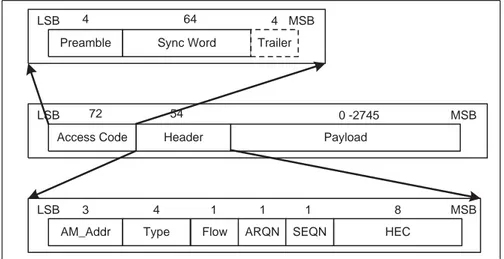
Bluetooth packets consist of three parts: Access Code, Header, and Payload. Each of these three parts also have sub-fields. Packets are send in little Endian format. As can be seen in Figure 2.3[2] least significant bit is on the left side and it is the first bit emitted to the air.
Access Code Header Payload
72 54 0 -2745
LSB MSB
Preamble Sync Word Trailer
4 64 4
LSB MSB
AM_Addr Type HEC
3 4 1
LSB MSB
Flow ARQN SEQN
1 1 8
Figure 2.3: Data Packet Content
The access code part is 72 bits if it is followed by the header, otherwise it is 68 bits long. The access code is the same for all packets sent in a piconet; it is the identification of the piconet of a packet. The access code is also used in protocols for constructing piconets as identification of nodes that are involved in the construction process. There are three types of access codes:
• Channel Access Code (CAC): The access code used as part of data packets during data transmission. It is 72 bits long.
• Device Access Code (DAC): The access code used during piconet formation processes. It is 68 bits.
• Inquiry Access Code (IAC): The access code used during inquiry process, as an identification of a single node that wants to join the piconet. It is 68 bits long.
The access code is composed of three fields:
• Preamble: Fixed zero-one pattern (0101 or 1010) to indicate the beginning of a packer and facilitate the reception of the packet.
• Sync word : The field that is used for identification purposed. The value of this field is derived from the hardware (Bluetooth) address of either the master or a slave. In CAC type of access codes, the value is derived from the hardware address of the master of the piconet. In DAC and IAC type of access codes, which is used during inquiry and page procedures, it is derived from the hardware address of the slave node that will join to the piconet. • Trailer : Fixed zero-one pattern to indicate the end of the access code.
The Header is the part of a packet that defines the target node, and the ordering and acknowledging information of multiple packets sent between pairs. In Figure 2.3[2] the length of header is shown as 18 bits. Error coding of header with 1/3 FEC results with a 54 bits long header. A header is composed of six fields:
• AM ADDR: Identifies the member address of the target node. When a slave is sending a packet to the master, slave uses its AM ADDR as in the case of master sending a packet to that slave. The all zero AM ADDR is used for broadcasting.
• Type: Defines the type of the packet that is sent. Type value indicates the number of slots that the packet will occupy and also also the type of the data (SCO or ACL data) that is carried inside the payload field.
• Flow : Defines the receive buffer availability of the receiver. • ARQN : Used for acknowledgment of previously received packets. • SEQN : Used for numbering of streamed packets
• HEC : Used to check header integrity.
The payload part of a packet is also divided into two subparts: payload header and data. The header of the payload may have two different sizes depending on the size of the packet in terms of time-slots that it occupies. For single-slot packets, payload header is one byte long. For multi-slot packets, payload header length is two bytes long. The payload header stores information about the length of the data that is stored in the payload part.
2.1.3.2 Packet Types
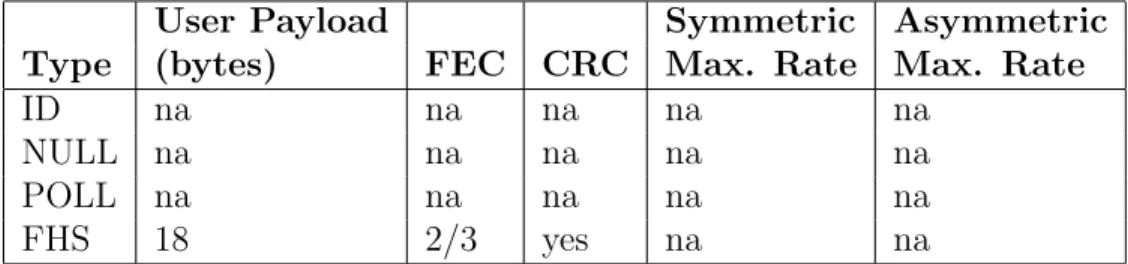
The type field in the packet header indicates the type of the content carried in the data portion of the packet payload. There are various packets: are four types of link control packets, seven types of ACL packets, and four types of SCO packets.
User Payload Symmetric Asymmetric
Type (bytes) FEC CRC Max. Rate Max. Rate
ID na na na na na
NULL na na na na na
POLL na na na na na
FHS 18 2/3 yes na na
Table 2.2: Link control packets
ID packets are used during device discovery and piconet construction process. These packets have only a header part. They are 68 bits long.
NULL packets have no payload and they are used for acknowledging previously received packets. They also carry information about the status of buffer at the receiver side. Total length of a NULL packet 128 bits. NULL packets are not acknowledged by the receiver of them.
POLL packets are similar to NULL packets in terms of format. POLL packets are sent by the master node of a piconet to the slaves in the piconet. They are used to indicate which of the slaves will use the next time-slot. Namely, they are used for reserving the next time-slot. A Polled slave must answer to POLL packets even through it has not data to send.
FHS packets are control packets that are use in many operations. FHS packets are sent as response messages during piconet construction. They are also used for piconet management and maintenance. FHS packets are single slot packets with a payload length of 240 bits.
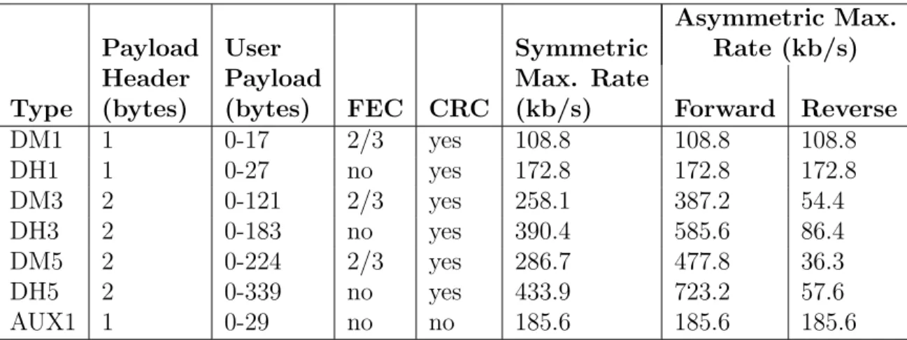
Asymmetric Max.
Payload User Symmetric Rate (kb/s)
Header Payload Max. Rate
Type (bytes) (bytes) FEC CRC (kb/s) Forward Reverse
DM1 1 0-17 2/3 yes 108.8 108.8 108.8 DH1 1 0-27 no yes 172.8 172.8 172.8 DM3 2 0-121 2/3 yes 258.1 387.2 54.4 DH3 2 0-183 no yes 390.4 585.6 86.4 DM5 2 0-224 2/3 yes 286.7 477.8 36.3 DH5 2 0-339 no yes 433.9 723.2 57.6 AUX1 1 0-29 no no 185.6 185.6 185.6
Table 2.3: ACL packets
ACL packets are used for carrying data. They can be sent regularly at specific time-slots or randomly at any time-slot provided that those time-slots are not reserved for SCO links. ACL packets can be retransmitted. The data they carry is usually not time-critical. A CRC mechanism is used to detect the errors on ACL packets.
messages. DM1 packets are the only packets recognized and used in both SCO and ACL links. The data stored in the payload portion of a DM1 packet can have a maximum length of 18 bytes and it is 2/3 FEC encoded.
DH1 packets are similar to DM1 packets except the payload is not FEC encoded. Each DH1 packet can carry up to 28 bytes of user data.
DM3 packets are three-slot packets with 2/3 FEC protection. Payload header in DM3 packets is 2 bytes. DM3 packets can carry 123 bytes of user data in their payload parts.
DH3 packets are similar to DM3 packets except the payload is not FEC encoded. Each DH3 packet can carry up to 185 bytes of user data.
DM5 and DH5 are five-slot data packets with the same properties as DM3 and DH3 packets, respectively. DM5 packets have a maximum data size of 226 bytes and DH5 packets have a maximum data size of 341 bytes.
AUX1 packets are similar to DH1 packets, but they do not have CRC. AUX1 packets can carry 30 bytes of user data in their payload.
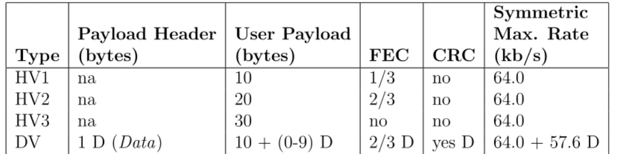
Symmetric
Payload Header User Payload Max. Rate
Type (bytes) (bytes) FEC CRC (kb/s)
HV1 na 10 1/3 no 64.0
HV2 na 20 2/3 no 64.0
HV3 na 30 no no 64.0
DV 1 D (Data) 10 + (0-9) D 2/3 D yes D 64.0 + 57.6 D
Table 2.4: SCO packets
SCO packets are used for time-critical applications like voice. The FEC coding on SCO packets are used to recover from bit errors. FEC is only mechanism for error correction on voice packets, since voice packets are not retransmitted when they are corrupt. To decrease the need for retransmission, SCO packets use higher-rate FEC protection.
An HV1 packet is a single-slot SCO link packet with high-rate error control. HV1 packets are protected with 1/3 FEC and can carry 10 bytes of voice data which makes the payload 240 bits long (10*8*3). An HV1 packet carries 1.25 ms of voice data. HV1 packets are sent every two time-slots as one time-slot is 0.625 ms and an HV1 packet can carry enough data for twice of this time.
An HV2 packet has the same size with HV1 packet but has less redundancy for error correction. HV2 packets carry 20 bytes of voice data with 2/3 FEC for error correction. An HV2 packet can carry 2.5m s of voice data, so HV2 packets are to be sent with a period of four time slots.
An HV3 packet has the same size with HV1 and HV2 packets but has no error correction bits included. An HV3 packet can carry 30 bytes of voice data with no FEC encoding. An HV3 packet can carry 3.75 ms of voice, so HV3 packets are to be sent with a period of six time-slots.
A DV packet carries a combination of voice and data payloads. The 230 bits payload is divided as 80 bits of voice and 150 bits of data. The DV packets are sent regularly like other SCO packets, but data and voice parts in the payload is processed differently. Voice part of the payload is treated as like other SCO packets and therefore they are never transmitted. Data part of the payload is checked for any errors, and it can be retransmitted if needed.
2.1.4
Connection Establishment and Piconet Formation
In Bluetooth, connecting two devices and forming a piconet has the same protocol. The protocol specifies the procedures that needs to be executed to connect two devices together and form a piconet of two nodes. The same procedures are used to connect a new node to the piconet. But specification of methods to inform all nodes about each others is left open to be investigated as part of the higher layer and applications.
A group of nodes (up to eight) that have established a shared link with each other is called a piconet. The frequency hopping sequence of the piconet, which
has to be followed by all nodes of the piconet, is determined entirely by the device address (BD ADDR) of the master of the piconet. The clock of the master determines also the phase in the hopping sequence. The master also controls the access to the shared frequency hopping channel that is used by the piconet nodes. The scheme that master uses for channel access is TDMA (Time Division Multiple Access). Master can use any scheduling algorithm in its implementation of TDMA scheme to provide different data-rates to the slaves while using the shared channel. In its simplest form, the master applies round-robin scheduling which dictates each slave to be polled one after another.
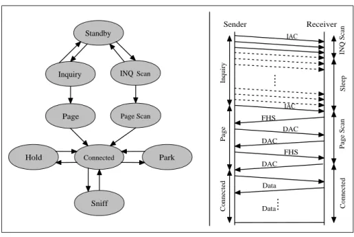
The state machine that is used while establishing a Bluetooth connection (link) between two devices is shown in Figure 2.4[2]. This state machine is ex-ecuted by both of the nodes involved in connection establishment. A Bluetooth device is in Standby state in default condition. In this state the device does not have any Bluetooth connection with any other device. The device may leave this state and start the procedure to connect to another Bluetooth device in range.
Standby Inquiry Page Connected Park Hold Sniff INQ Scan Page Scan Sender Receiver IAC .... IAC Inquiry INQ Scan Sleep FHS DAC DAC FHS DAC Page Scan Page Connected Connected Data Data....
Figure 2.4: Connection States
There are two options that a device uses to make an attempt to connect to other devices in the region. In the first option, the device can start sending inquiry
messages. This is an attempt to discover other nodes in the region and connect to one of them. The node that sends inquiry messages also assume the role of master in the piconet that is to be established by itself and another node answering the inquiry. This state where the node sends inquiry messages is called Inquiry state. An inquiry message that is sent in this state is composed of device’s Inquiry Access Code (IAC). This code enables another unit receiving inquiry message to learn the sender’s identification. Different from sending normal data packets, a unit sending an inquiry message jumps through 16 frequency channels (hops) and sends the inquiry message in all these channels. After sending this sequence of 16 messages, the sender listens the channel for a response. The sends jumps through 32 channels from which a response is possible to come. The response, when it comes, includes the identification of the node sending the response. In this way, the node that initiates inquiry will learn about the nodes in the region to whom it may connect.
The other option for a device to to attempt to make a connection to another device is looking for inquiry messages. For that, the device enters into the Inquiry Scan state and listens the channel for inquiry messages. When the device enters inquiry scan state, it also assumes the role of slave in the connection that can possibly be established. As Bluetooth units follow a pseudo-random sequence of frequencies (as a requirement of frequency hopping scheme) to transmit packets, in order to increase the probability that two nodes in Inquiry and Inquiry Scan states to meet at the same frequency, they apply different timings during the states and scanning procedures. The node in Inquiry Scan state listens for 32 channels long enough so that the other node in Inquiry State jumps through 16 channels.
If here are several devices in the region of a node that sends an inquiry mes-sage, a contention may occur when those devices would like to respond back. To prevent this, a device that receives a inquiry message waits a random amount of time in sleep mode and then wakes up and waits for an other inquiry message to arrive. When the message arrives, the nodes send an reply back immediately. The reply is a FHS packet. The FHS packet contains information about the frequency hopping sequence and clock of the node.
Step Message Direction Hopping Sequence Access Code
1 ID master to slave inquiry inquiry
2 FHS slave to master inquiry response inquiry
Table 2.5: Inquiry, Inquiry Scan messages
The unit sending the FHS packet leaves the inquiry scan state and moves into Page Scan state. The receiver of the FHS packet leaves the inquiry state and moves into Page state. In these phases, the initiator of the connection (the sender of inquiry message - master) has information about the hopping sequence of the other unit (the receiver of inquiry message - slave). Initiator unit uses this hopping sequence information to adjust its carrier frequency to match to the carrier frequency of the slave). After that, the master sends a DAC message that contains information about the receiver in the access code part of the message.
Table 2.6[2] shows sequence of messages (control packets) that are exchanged between two nodes that would like to establish a Bluetooth connection. One node assumes the role of master and the other one assumes the role of slave. After a connection is established, the frequency hopping sequence of the master is used as the hopping sequence of the connection, i.e. the slave also follows the same hopping sequence while jumping from one frequency to another.
Hopping Access Code
Step Message Direction Sequence and Clock
1 Slave ID master to slave page slave
2 Slave ID slave to master page response slave
3 FHS master to slave page slave
4 Slave ID slave to master page response slave
5 1st packet of master master to slave channel master
6 1st packet of slave slave to master channel master
Table 2.6: Page, Page Scan messages
When a device is connected to another node or to a piconet, the unit can operate in one of the following states: active, hold, and park. Being in different states is useful for energy efficiency and effective channel utilization. When device
would like to send or receive data, then it operates in active state. In active state, the device is an active member of the piconet. An active member has a unique identified in the piconet (called AM ADDR) that is used as the address of the device. AM ADDR is 3 bits long.
A device can save energy even it is in active state. This is possible by going into sniff mode and listening to the channel periodically if there is a transmission from the master to that device. These time-slots, when the device listens to channel are called sniff time-slots. The period of sniff time-slots is negotiated between the master and slaves. A device is asleep in time-slots other than the sniff-times slots if it is not sending or receiving data. At the beginning of a sniff time-slot, a device that is sleeping wakes up and listens for a Bluetooth packet to arrive. When packet arrives, it decodes the AM ADDR fields and checks if the value is same with its 3-bit address. If they are the same, the device continues to listen and receives the packet. Otherwise, the device goes to sleep immediately until the next sniff time-slot.
An active member of a piconet can get into hold state. In hold state, a device keeps its AM ADDR with the piconet. Hold state is a power saving mode where the unit can switch to other frequency hopping sequences for a period of time (to take part in other piconets), or switch to power saving mode. Another power saving mode that a device can be in is Park state. In park state, the device gives its AM ADDR back, and does minimum task just to keep synchronized with the piconet. A device can switch to active state from sniff or hold states at any time. But a device has to get a new AM ADDR from the master of the piconet, if it would like to switch to active state from park state.
2.1.5
Constructing and Operating Scatternets
The procedures for how to construct (form) scatternets is not specified in Blue-tooth standards and is left as an open research issue. There are mechanisms describes in standards that enable formation of scatternets. A scatternet has to be formed from piconets. Multiple piconets are inter-connected with each other
through some special nodes of those piconets, that are called bridge nodes. A bridge node can be member of multiple piconets at the same time and it takes the responsibility of forwarding inter-piconet traffic between those piconets. Fig-ure 1.2 shows an example scatternet and a bridge node.
A bridge can not be active in multiple piconets at the same time. Therefore, it takes turns in participates in multiple piconets. While being active in one piconet, it has to be in sniff, hold or park mode in the other piconet. After staying active in that piconet for some time, the piconet switches to the other piconet to become active in that piconet. A bridge node can take master role only in one piconet, but can take slave role in multiple piconets. When a bridge node takes the master role in one piconet, the traffic in that piconet is suspended during the time that that bridge switches to an other piconet, since a piconet can not operate without a master. It is possible that bridge node take the slave role in all the piconets that it participates.
Besides the problem of constructing scatternets, there are also other issues related with scatternets that needs to be discussed briefly. One issue is discovery of devices that comprises a scatternet. How a device can learn the identity of another device that is in the same scatternet but in a different piconet? Another issue is related with identification of devices. How can we identify the devices uniquely while sending packets to them? In a piconet, AM ADDR is used as destination address in packets. But an AM ADDR is 3 bits and therefore can address at most eight different devices. However, a scatternet can consists of any number of nodes without any limit. Therefore use of AM ADDR is out of con-sideration. There are two other alternatives remaining. One is using Bluetooth device addresses (which are 48-bits long) as the destination address in packets. The other is use of IP addresses, which requires assignment of unique IP addresses to each device. This also raises the question of how to assign unique IP addresses automatically to Bluetooth devices. The assignment can be arbitrary or in a way that can facilitate easy and efficient routing as in Internet now.
One other problem with scatternets is how to route packets between nodes in a scatternet. Should we forward and route the packets at layer-2 (data-link layer)
or layer-3 (network layer) of protocol stack. The choice also affects the method to be used to identify devices. If we forward packets at layer-3, this implies that we have to use IP addresses as the destination address in the packets. This requires assignment of a unique IP address to each node. Although there are various efforts in solving the routing problem for ad-hoc networks [8][9][10][11][12], these solutions may not be directly applied to Bluetooth scatternets in an efficient manner. Then, either one of these solutions has to be enhanced to support Bluetooth topologies which have different characteristics than random ad-hoc network topologies, or a brand new solution for Bluetooth scatternets has to be developed.
In our study, we focus on the problem of how to construct a Bluetooth scat-ternet in a way that the scatscat-ternet is efficient in operation, i.e. while carrying user traffic. Since we expect the efficiency to be dependent on the pattern of user traffic that will flow in the scatternet, we take a proactive approach and consider the traffic pattern in the establishment of the scatternet as an input to the construction algorithm. Our work differs from most other works in this issue by focusing on the efficiency of the constructed scatternets, rather than focusing on the efficiency of the construction algorithms.
2.2
Related Work
There are many ways to focus on the problem of Bluetooth scatternet construc-tion. Most research work so far have focused on the performance of the algorithms for scatternet construction. Some of them try to reduce the running-time of the algorithms, so others try to reduce the implementation and message complexity of the algorithms. Some other research work has focused on the finding algorithms that generated topologies on which efficient routing of packets between nodes is possible.
In their studies C. Law and K.Y. Siu [13] [14] define the performance metrics for Bluetooth scatternet formation as the duration of scatternet construction
process and the number of control messages exchanged during this time. They objective of construction is to reach to a topology that has the least number of piconets possible. They claim that decreasing the number of piconets decreases the interference that piconets cause to each other due to narrowband frequency collisions and also the diameter of the resulting network.
But contrary to Law’s claim, Zurbes [6] shows that increase in frequency collisions in a scatternet while the number of piconets comprising the scatternet increases do not actually decrease the performance and total capacity of the network. His experiment results indicate that until the number of piconets reaches to a threshold number, which is 60, the total capacity of the network increases. This is because each piconet that is added to the scatternet adds also new capacity to the scatternet (since each piconet is using a different frequency hopping channel and this enables simultaneous communication with other piconets), although it slightly increases the probability of interference that is still possible between frequency hopping channels. Additionally, increasing the number of piconets decreases the intra-piconet traffic on each piconet, since there will be less number of nodes per piconet in when we increase the piconet count. Reducing the number of nodes per piconet will result in reduced scheduling and packet delays in traffic flowing between nodes of a piconet.
Salonidis et al [15] define other metrics to evaluate the performance of scat-ternet construction algorithms. These metrics are connection set up delay and probability of protocol correctness. They also propose a scatternet formation algorithm called Bluetooth Topology Construction Protocol (BTCP) which aims to be a distributed protocol. But in their protocol, only the coordinator selec-tion process is distributed. Once a coordinator is selected, it is responsible from forming the scatternet in a centralized way.
BTCP has three phases:
1. A coordinator is elected
2. The coordinator determines the roles of other nodes in the scatternet to be constructed.
3. The scatternet is constructed according to instructions of the coordinator.
BTCP’s assumption of Bluetooth devices will try to connect to each other nearly at the time contradicts with the fact that Bluetooth is an ad-hoc wireless technology where nodes may join or leave the network at any time, dynamically. Therefore, BTCP is not a dynamic algorithm and does not support new devices to join a network at any time or a device to leave the scatternet at any time. IN short, it does not provide any mechanism to maintain the network after setting up the network. BTCP is one of the first studies in the area scatternet construction, and therefore it is an important contribution.
Another study by [16] Zaruba and Basagni do not state a specific performance measure for network topology. Their goal is to construct a tree-shaped scatternet and they claim that routing will be more efficient on a tree-shaped topology. However, they ignore the potential bottleneck problem in the root or in close-to-root nodes of the tree in case of a high traffic demand between distant leafs of the tree. Also the proposal lacks the property to deal with ad-hoc structures. Within a tree structure, connection can easily be lost in case of a node leaving the tree. A tree-based solution is proposed also by other researchers. In his study, Tan [17] is using two performance metrics regarding scatternet formation and evaluation of the resulting topology: 1) scatternet formation time, and 2) average end-to-end latency in traffic flows. The main reason for using tree structure is stated as simplifying routing and scheduling. The possible bottleneck problem in root nodes is also ignored in this research.
Other studies propose some other topological structures. BlueStars [18], BlueMesh [18] are example studies that propose different structures. They aim to have scatternet topologies where there are multiple paths between pairs of nodes. This will increase the fault-tolerance of the topology. They also put some constraints on the number of nodes that a piconet can have. Their studies are practical enough to be applied within current Bluetooth specification constraints. There are other studies that guided us in formulating our problem. Bhagwat [19] and Kalia [20] have substantial amount of work in this field, from which we
have benefited. Kalia, in his study about the performance of inter-piconet traf-fic in different scatternet architectures, show the power of multi-path connected network topologies over tree-based structures. Bhagwat discusses the constrains that should be considered while designing scatternet formation algorithms.
As we can observe in the previous studies, some of them have focused on scatternet set-up time and complexity of the construction algorithms in terms of control messages exchanged. Some of the studies also focus only on the construc-tion of the scatternet, but maintenance of the resulting scatternet is ignored. This is not acceptable since Bluetooth technology supports ad-hoc networking scenarios where nodes may join or leave a scatternet at any time. Also none of the previous work considers much the efficiency of the resulting scatternets in terms of end-to-end packet delays, scatternet utilization, bandwidth guaranties, etc. We believe that efficiency of a scatternet topology in terms of these metrics is highly dependent on the pattern of the traffic that is flowing in the network, i.e. traffic requirements of nodes among each other. Therefore, a solution for scatternet construction should take into account the possible traffic requirements of nodes among each other before constructing the scatternet. In its simplest form, the nodes that communicate heavily with each other should also be placed close to each other in the scatternet.
We took this observation as the basis of our research and we proposed a scat-ternet formation algorithm that considers the traffic requirements (demands) of the nodes into account while constructing the scatternet. We show that a scat-ternet constructed in this way performs better in terms of performance metrics like weighted average shortest path (WSP), network utilization (TU), and sat-isfiability of user traffic demands (BR). In the following chapters, we will first describe our performance metrics (WSP, TU, and BR), and then we will describe our algorithm in detail. Then we will provide our simulation results that evaluate the performance of our algorithm in terms of the metrics that we have defined.
Scatternet Formation Algorithm
3.1
Performance Metrics for Scatternets
In many of the algorithms for Bluetooth scatternet formation, running time and implementation complexity of construction algorithms are main performance met-rics. One main objective is usually to decrease battery usage during construction. To some extent this point of view is correct, but when battery life is considered, energy consumption in the constructed scatternet is at least as important as the energy consumed during construction.
Here we offer performance metrics that can be used to evaluate the efficiency of the constructed scatternets, not the construction efficiency of the scatternets. Our performance metrics are similar to metrics of Wang in his studies of Bluenet [21], but different from Wang’s study we consider each traffic flow path with its data traffic amount as its weight coefficient, whereas Wang accept all flows as the same. In their study, Average Shortest Path (ASP) and Maximum Traffic Flow (MTF) are used for evaluation. Here we consider Weighted Average Shortest Path (WSP) and Topology Utilization - Blocking Ratio (TU-BR), respectively. Our performance metrics are designed to express the efficiency of the scatternet for satisfying end-to-end traffic demands between pairs of nodes and to show the portion of the bandwidth capacity used as a result of the traffic demand.
Weighted Average Shortest Path (WSP) of a scatternet is computed as follows. For each flow fx, the length of the path that flow traverses is multiplied by the weight of traffic flow fx. The weight of traffic flow is computed as the ratio of the demand of the flow to the total traffic demand. During calculation of WSP, shortest possible paths of flows and average traffic demands between pairs are used. In a real life situation paths may be longer, but effect of routing on the performance is beyond the scope of this thesis.
More formally, if there are n flows where each flow has a traffic demand of di then WSP for flow fx is:
W SPx = dx P
1≤i≤ndi
× Lx, (3.1)
where Lx is the length of the path (in hops) that flow fx is traversing to reach from source to destination.
Then the WSP for a scatternet with n flows is:
W SP = Pd1 di × L1+ d2 P di × L2+ ... + dn P di × Ln = P 1 1≤i≤ndi (Pn i=1di× Li) or W SP = Pn i=1diLi Pn i=1di (3.2) Example: X T M N Z L K
Assume we have 3 flows:
F1: X - Z - K d1= 10, L1= 2
F2: T - Z - K - L - M d2= 25, L2= 4
T otalDemand = 30 + 25 + 10 = 65 W SP1 = 2 × 1065 W SP = 10.2+25.4+30.3 65 = 210 65 = 3.2 (3.3)
Average Shortest Path metric proposed by Wang et al. [21] uses average path lengths, but we also consider the effect of date rate of each flow. ASP treats all data flows similarly, but two data flows of 1 Kbps and 700 Kbps of data-rate put different loads on the scatternet. When data flows have similar traffic rates, WSP and ASP will show similar results. Their difference is witnessed as the variance of traffic rate of flows increases.
In our research, traffic rates of flows is given importance because mobile de-vices spend their energy resources for receiving and sending packets. The amount of power consumed by a mobile device is proportional to the rate of packets that are transmitted or received by that mobile device. In other words, the energy consumed by a mobile device is related with the number of packets that the mo-bile device transmits or receives. In order to optimize the system considering the traffic demands (i.e. requires traffic rates of flows), paths of high-demand flows should be shorter so that less number of intermediate nodes will be busy to use their resources for these flows. WSP of a topology is an indication of how far the end-points of flows are placed from each other in a scatternet. When flows with higher traffic demands have been placed close to each other, i.e they travel shorter paths, then their WSP total also be smaller. The smaller the WSP total is, the less will be the overhead of highly active flows on intermediate nodes.
TU-BR metric depends on topology utilization and blocked traffic ratio. TU part of the metric is obtained by taking the ratio of the total traffic flowing in the system to the possible maximum capacity that can be provided by the topology. When the TU is high and satisfaction of end-to-end demands is at an acceptable level, it shows that the scatternet constructed is in coherence with the traffic demands of the nodes.
Topologies constructed must provide an acceptable level of service to partici-pating nodes. The level of service can be expressed with BR. The topology must be constructed so that the traffic demands of flows can be carried over designed topology. For some topologies some of the flows cannot be satisfied due to:
• Bottleneck links whose capacity is reached and therefore can not carry any more flows that have to go over this link.
• Bottleneck nodes whose in - and out - traffic demands is beyond limits of forwarding capacity of the node.
Zurbes [6] shows that total capacity of scatternet increases as the number of piconets constituting the scatternet increases. The increase in capacity continues until the number of piconets reaches to a threshold value where capacity loss as a result of interference between piconets overweight the capacity increase. We omit the effects of possible interference and also scheduling conflicts in resulting topologies, as the possible number of nodes we plan to serve are far below this number. The maximum total capacity of a scatternet can be found by applying a bipartite matching algorithm on the resulting scatternet topology. In this way, the maximum traffic amount that can be carried at a given moment can be obtained. For simplicity, we take the number of piconets as a measure for capacity. Using this simple approach, if there are n piconets, we consider the capacity of the scatternet as n * 1 Mbps.
There is a computational cost for running a scatternet formation algorithm that considers traffic demands of nodes’. The primary goal of this thesis is to show that performance gained with such an algorithm outweighs the costs associated with the algorithm.
3.2
Scatternet Formation with Traffic
Consider-ation (FTC) algorithm
3.2.1
Overview
This thesis is a part of a research effort for designing effective and feasible scatter-net construction algorithms. Towards having a complete solution for scatterscatter-net formation, we planned to follow a step-by-step approach. First, we aim at deriv-ing performance metrics that can be used to evaluate the generated scatternet topologies. Then, we develop an algorithm that creates Bluetooth scatternets based on traffic demands. Then, we evaluate the topologies that have been gen-erated with our algorithm using our metrics for evaluation.
With our work we also would like to see if the effort to construct these topolo-gies is justified with the gain we obtain by using these topolotopolo-gies to transport user traffic.
In the first phase of our research, we have made some assumptions that will facilitate modeling the problem. Like many other work in literature, we assume that all nodes in a scatternet are visible to each other in terms of radio connec-tivity and they are aware of each other so that they can send or receive data to or from each other. Scheduling algorithms for intra-piconets and inter-piconet communication is beyond scope of this study, as well as the routing of packets for inter-piconet flows. We assume that packets are using the shortest paths available.
Besides providing a solution for scatternet construction, we also analyze our solution and scatternet construction approach. In our evaluation, we have a group of nodes and traffic flow information between these nodes. We first aim to show that a topology that is constructed according to traffic demands achieves a better performance, and the cost of such a construction is justified. In future solutions we plan to modify our solution to handle real-life traffic scenarios.
In our solution approach there are some issues that need to be discussed first before providing the solution. The method that can be used to gather traffic flow data, and the selection of master and bridge nodes are among these issues.
3.2.2
Traffic information
The information about data traffic flowing between nodes can be obtained by using one of several possible methods. One method is examining the logs of wireless network activity if such logs are kept by the system. Another method is monitoring the traffic flow in real-time and estimating the traffic parameters of flows. These parameters may include the average bit-rate, average packet size, etc. For the specific case of Bluetooth networks, traffic can be monitored at master nodes of piconets, since all data traffic in a piconet passes through the master node. The average rate of traffic (in Kbps) can be obtained by using an aging algorithm described with Equation 3.4. This aging method relates the instantaneous traffic rate to the average traffic rate using an aging factor α, that is between zero and one. This average rate of flowing traffic can be used for topology modification, scheduling and even for routing. The traffic rate can also be expressed in number of time slots used by a flow in a second (time-slots/second). In the initial construction of a scatternet, there will be not enough data to infer traffic parameters. But as time passes, enough data will be available to estimate the parameters. The rate of a flow may change from time-to-time. With the help of the aging method, the changes are transformed into data in a smooth linear curve which is better compared to working with snapshots.
AvgRatet = (α ∗ AvgRatet−1) + (1 − α) ∗ InstRatet
0 ≤ α ≤ 1 (3.4)
3.2.2.1 Traffic quantities
In our algorithm we use traffic flow rate values that are integers. The traffic rate of a flow is expressed by the number of time-slots needed in a second by that
flow. The length of a time slot in Bluetooth is 625 µsec, so there are 1600 time-slots per second for Bluetooth devices. A Bluetooth device can send or receive at most 1600 data packets per second and also the maximum capacity of a shared Bluetooth channel (i.e. piconet capacity) is 1600 slots per second. There may be at most 1600 packets/sec in a shared channel. In our experiments we use the number of sots needed per second as the unit of flow rate (or amount). We assume that the biggest possible packet size (out of sizes 1, 3 and 5) is used for transmission so that we can have good channel utilization.
3.2.3
Master selection
Master selection is an important issue that affects the power efficiency of a pi-conet and performance of scheduling. For a given traffic flow data for a pipi-conet, there may be varying results for power consumption depending on which node is selected as the master.
Given a set of nodes in a piconet and the traffic demand values between them, flows in the piconet can be divided into two:
• Master-to-Slave or Slave-to-Master flows: TM →S, TS→M • Slave-to-Slave flows: TS→S
From these flows we can compute two cumulative values:
• Total Demand : the total amount of traffic demands. This is a fixed amount with a given traffic demand information for the piconet.
• Total Load : the total amount of traffic load on scatternet as a result of traffic demands. This value shows the used capacity of the piconet. The smaller this total is, the less will be the energy and bandwidth consumed in the piconet. Reducing the bandwidth consumption due to intra-piconet traffic, leaves more remaining capacity for inter-piconet traffic. This helps
in finding a feasible scheduling policy for intra-piconet and inter-piconet traffic.
Total traffic demand in a piconet is independent of assignment of master and slave roles to the nodes in the piconet:
T otalDemand =XTS→S+ TM →S+ TS→M (3.5)
Total traffic load depends on total demand and also on the assignment of master and slave roles to the piconet nodes:
T otalLoad =X(2 ∗ TS→S) + TM →S + TS→M (3.6)
Equation 3.6 is a result of Bluetooth piconets’ having star topology (see Figure 1.3). Connections between slave and master nodes of a piconet have one hop path lengths. Packets sent from master node to slave nodes pass the wireless channel only once, and this is also true for packets traveling in opposite direction. As a result of this, M → S and S → M connections put a load on system that is equal to their traffic demands. However, communication paths between slaves of the same master are two-hop paths. Therefore, S → S communications create a load on piconet that is twice of their traffic demands.
In order the decrease total load on a piconet, we need to decrease the TS→S in equation because the rest of the equation is fixed. When roles in the piconet is distributed in a way so that sum of TM →S and TM →S gets maximum, then TS→S gets its minimum value. In other words, when we select the node which has the highest total traffic demand as the master node, total load on the piconet is minimized. This result is also stated in the study of [20]. When the most active node is selected as the master it is easier for that master to schedule the traffic in the piconet because it has the most accurate information about flows in the piconet as it is involved in many of these flows.
The method described above is used to select the master node of each piconet. In this way, the load on each piconet is decreased, hence the load on the scatternet.
Master selection is repeated with every change of topology of a piconet , such as addition/deletion of a member node. In an algorithm to be developed for real-life traffic scenarios, periodic controls need to be done to dynamically adjust to changes in traffic. Some of the changes may be significant enough to trigger the master selection process.
During master selection, bridge nodes of piconet are not considered as candi-dates of being the master. When a bridge node would take the role of being a master in a piconet, the traffic in that piconet will be suspended during the time that the bridge node has switched to its role in the other piconet. There may be cases where a master node has a traffic flow pattern that suggests that master to be a bridge node, but we give more importance to intra-piconet traffic than the inter-piconet traffic.
3.2.4
Bridge selection
One other important procedure that we define in scatternet formation is bridge selection among slave nodes. Master nodes are not given bridge functionality because when the master of a piconet switches to another piconet, all traffic needs to be suspended. Also when a node would take the responsibility of being both a master and a slave in a scatternet, it has to coordinate both intra-piconet and inter-piconet scheduling, which will put more computational load on the node. Therefore, we only use slave-slave type of bridges in our solution. A slave-slave bridge takes slave roles in both the piconets that is connected to. One other reason for using only slave-slave bridges is to prevent tree-like topologies in our scatternets, since in the root node in a tree-based topology has potential to be a bottleneck.
Bridge nodes are selected according to their suitability to be an intermediate node that carries inter-piconet traffic. When there is a need for a bridge between two piconets, we search among slaves of both piconets for slaves that are not bridges already. During the search we look to the total traffic demands to nodes of other piconet and also to the total traffic demands to nodes of the original
piconet. We select the node with highest total traffic demand with nodes of other piconet and lowest demand with the nodes of its own piconet. In this way, we try to localize the flow of traffic and shorten the path length of traffic flows. Bridge nodes operate by being member of both piconets. When we select the node with highest cumulative traffic demand to other piconet, those traffic demands are satisfied as intra-piconet communication links where path lengths are at most two. Selecting a node with lowest intra-piconet cumulative aims to prevent bottleneck points in communication. Inter-piconet traffic scheduling is supposed to be easier for nodes that have less loads of intra-piconet traffic.
In current implementation, once a bridge node is selected between two pi-conets, we do not search for a possibly better bridge node when other nodes are added to piconets. This might be implemented in a dynamic distributed system and improve the performance of the system.
3.2.5
Maximum path length
Maximum path length is a parameter that has impact on performance. If two nodes are connected with a routing path that is greater than a threshold value (maximum path length), we consider these two nodes as disconnected and try to form a new route between them. This approach affects the connectivity dis-tances between nodes and WSP value. But there is a trade-off in selecting a maximum (threshold) value for path lengths. A small value will result with a highly connected topology which results in an increase in average responsibility given to nodes, in higher switching load, and more difficulty in finding a feasible scheduling policy. A large value for threshold value results with long path lengths where load on intermediate nodes tends to increase and lifetime of topology tends to decrease due to high power consumption during communication. Considering this trade-off, we initially set the maximum path length value to four, but this can be changed.