A Parallel Prolog emulator

A PARALLEL PROLOG EMULATOR

A THESIS

SUBMITTED TO THE DEPARTMENT OF COMPUTER

ENGINEERING AND

INFORMATION SCIENCES

AND THE INSTITUTE OF ENGINEERING AND SCIENCES

OF BILKENT UNIVERSITY

IN PARTIAL FULFILLMENT OF THE REQUIREMENTS

FOR THE DEGREE OF MASTER OF SCIENCE

By

Attila Giirsoy

JuR 19SS

Q f\

G 968^

I certify that I have read this thesis and that in my opinion it is fully adequate, in scope and in quality, as a thesis for the degree of Master of Science.

________ _________________________________ Prof.Dr.Mehmet Baray(^iincipal Advisor)

I certify that I have read this thesis and that in my opinion it is fully adequate, in scope and in quality, as a thesis for the degree of Master of Science.

I certify that I have read this thesis and that in my opinion it is fully adequate, in scope and in quality, as a thesis for the degree of Master of Science.

Inst.Işık Aybay

Approved for the Institute of Engineering and Sciences:

ABSTRACT

A PARALLEL PROLOG EMULATOR

Attila Giirsoy

M.S. in Computer Engineering and

Information Sciences

Supervisor: Prof.Dr.Melimet Baray

July 1988

There are various parallel Prolog execution models proposed so far. In this study, an emulator has been developed to test the execution model PPEM. The emulator is used to collect data to evaluate the performance of the model. The underlying architecture is assumed to be a tightly coupled multiprocessor system. Some implementation difficulties faced, which are not apparent in the definition of PPEM are discussed, and performance results are presented.

Keywords: Prolog, Logic Programming, Emulators, Parallel Processing, Parallel Prolog.

ÖZET

PARALEL PROLOG EMÜLATÖRÜ

Attila Gürsoy

Bilgisayar Mühendisliği ve Enformatik Bilimleri Yüksek Lisans

Tez Yöneticisi: Prof.Dr.Mehmet Baray

Temmuz 1988

Şimdiye kadar, çeşitli parcilel Prolog işletme modelleri önerilmiş ve uygu­ lanmıştır. Bu çalışmada paralel Prolog işletme modeli PPEM için bir emülatör geliştirilmiştir. Emülatörün am acı, modeli test etmek ve performans çalışmalarında kullanılmak üzere veri toplamaktır. Ayrıca , modelin tanımında gözükmeyen bazı uygulama zorlukları ve ön performans sonuçları sunulmuştur.

Anahtar KelimelerrProlog,Mantıksal Programlama, Emülatör, Paralel İşlem, Paralel Prolog.

ACKNOWLEDGEMENT

I would like to express my gratitude to Prof. M.Baray for his supervision and support during the development of this thesis.

I also would like to thank Mr. Işık Aybay for his valuable discussions and comments.

TABLE OF C O N TE N TS

1 IN T R O D U C T IO N 1

1.1 Parallel P r o l o g ... 1

1.2 Purpose and Scope of the T h e s i s ... 2

2 Parallelism in Prolog 3 2.1 An overview of P r o l o g ... 3 2.1.1 Unification in P r o lo g ... 4 2.2 A N D /O R T re e s... 5 2.3 Search Strategy of P r o l o g ... 5 2.4 Parallelism in P r o lo g ... 6 2.4.1 OR Parallelism ... 7 2.4.2 AND Parallelism ... 8

2.5 Parallel Prolog Execution Model P P E M ... 11

2.6 Parallel Architectures ... 13

2.6.1 Array P rocessors... 14

2.6.2 Multiprocessors... 14

2.6.3 Data Flow M ach in es... 16

3 Implementing A N D /O R Parallelism 17 vi

3.1 A N D /O R Process ... 17 3.2 AND Parallelism ... 19 3.2.1 Execution of a C hain... 20 3.2.2 Join O p e ra tio n ... 22 3.2.3 Duplicate Bindings... 24 3.2.4 Cartesian P r o d u c t ... 27 3.3 OR Parallelism ... 30 3.3.1 Pipelining... 30

3.3.2 Some improvements in OR processes... 31

4 ST R U C T U R E OF THE E M U L A T O R 33 4.1 Parallel Prolog Emulator... 33

4.2 System Parcimeters... 34

4.3 T im ing... 35

4.4 Performance M easures... 36

4.5 Model of the A rch itecture... 36

4.6 Intermediate C o d e ... 38

4.6.1 Translation from Prolog to Intermediate c o d e ... 38

4.6.2 Built-in F u n ctio n s ... 41

4.6.3 Playing with G ra n u la rity ... 42

4.7 Data structures for bindings... 43

4.7.1 Representation of t e r m s ... 43

4.7.2 Basic Data Types ... 45

4.7.4 Bindings containing unbound variables... 51

4.8 System Related Data Structures 52 4.5.1 Clause table... 53 4.8.2 Process Representation 53 4.8.3 Processor l i s t ... 56 4.9 Communication... 57 4.10 OR p r o c e s s ... 59 4.11 AND P r o c e s s ... 60 4.12 Results... 62 5 Conclusion 70 REFEREN CES 72 A P P E N D IX 75 A Test Programs 75

LIST OF FIGURES

2.1 Unification of two t e r m s ... 4

2.2 A N D /O R tree... 5

2.3 Infinite b r a n c h ... 6

2.4 OR parallelism ... 7

2.5 Joining the results of two s u b g o a ls ... 8

2.6 Execution g r a p h ... 9

2.7 Execution of two set of subgoals ... 12

2.8 Tightly coupled multii^rocessor s y s te m ... 14

2.9 Loosely coupled multiprocessor sy stem ... 15

2.10 Interconnection top ologies... 16

3.1 A N D /O R processes... 18

3.2 AN D /O R tree representation of the e x a m p l e ... 19

3.3 Graph for the ch a in s... 20

3.4 Execution of a c h a i n ... 21

3.5 The set S and T Z ... 22

3.6 Bindings when 1/ = 0 . . . . ... 23

3.7 Bindings when u ^ $ ... 24

3.8 Example 1 for j o i n ... 25

3.9 Example 2 for j o i n ... 25

3.10 Duplicate values in a s e t ... 26

3.11 Duplicate columns containing structures with variables . . . . 26

3.12 Joining duplicate structures... 27

3.13 Cartesian product operation... 29

3.14 Or p ip e lin in g ... 31

4.1 Parallel Prolog Emulator... 34

4.2 State diagram for F C F S ... ... 37

4.3 Blocking clauses in a p roced u re... 43

4.4 DAG representation of t e r m s ... 44

4.5 DAG representation of terms with offsets 45 4.6 The structure for a simple t e r m ... 46

4.7 Representation of a term-list 47 4.8 Implementation of term s... 47

4.9 Representation of l i s t s ... 48

4.10 Structure of unilist and g lis t... 49

4.11 Unification environment for a particular in s ta n c e ... 50

4.12 Representation of u n ir e s u lt... 50

4.13 Local variable table... 52

4.14 Ordering the va ria bles... 52

4.15 Structure of a p r o c e s s ... 54

4.17 Signal p a c k e t ... 57

4.18 Message ty p es... 58

4.19 Speedup r a t e ... 63

4.20 Speedup rate for different p s t ,p c t ... 64

4.21 Throughput of the system for s u b s e t ... 66

4.22 Average system utilization... 66

4.23 Granularity selection for program p 2 ... 67

LIST OF TABLES

4.1 Information collected by the Emulator 68

1. IN T R O D U C T IO N

1.1

Parallel Prolog

Conventional sequential processors axe unable to provide the necessary com­ puting power to problems in some fields like artificial intelligence which re­ quire very fast processing. There is a fundamental limit or technological limit to the amount and speed of computing and we are already getting closer to this limit. Increasing the speed and power of computers through methods that are beyond technological advances can be aclrieved by parallel process­ ing.

Prolog seems to be a suitable language for parallel execution because of its nondeterministic choices and easy decomposition into subtasks. Several methods have been proposed to improve the performance of Prolog so far. After Prolog was selected to be the basic language for the Japanese fifth generation project, studies on parallel execution of prolog has increased sig­ nificantly.

Generally, the most important sources of parallelism in Prolog are :

• OR parallelism, • AND parallelism.

and in AND parallelism, subgoals are evaluated concurrently.

1.2

Purpose and Scope of the Thesis

The aim of the thesis is to develop an emulator for the parallel Prolog ex­ ecution model PPEM [1] where the underlying architecture is assumed to be a tightly coupled multiprocessor ( i.e, shared memory) system which is defined in [1]. The idea behind the emulator is to check the consistency and understand all consequences of the model.

The execution model has not been implemented yet, so what is expected is an improved intuition about behaviour and essential aspects o f the execution model at the implementation stage.

In the next chapter, a survey of parallel Prolog is presented. Two basic types of parallelism in Prolog , OR parallelism, AND pcurallelism are dis­ cussed. The execution model is explained and some parallel architectures on which the model may be implemented are introduced.

In Chapter 3, implementation concepts of A N D /O R parallelism is dis­ cussed.

In Chapter 4, the structure and the implementation of the emulator is presented. Also some performance measurements are discussed.

2. Parallelism in Prolog

2.1

A n overview of Prolog

Logic programming is a general programming methodology based on the idea of theorem proving within the Horn clause subset of first order calculus, and Prolog is the implementation of this idea [20].

A Prolog program is a set of clauses . A clause is of the form

P ·(— Ai, A.2, . . . , Am

where P and A,· are atoms. P is called the head of the clause, the right side of the clause is called the body, and each A,· is a subgoal. An atom has the form p(^i, . . . ,tk) where p is a predicate name, and ¿,· is a term.

A clause with an empty head is called a query or goal and it represents the problem to be solved.

A clause with an empty body is called a fact.

A Prolog procedure is a collection of rules all having the same predicate name in their head.

A term is either a constant, a variable or a structure. All symbols begin­ ning with lowercase letters are constants. Variables starts with an uppercase letter. A structure tal^es the form

Figure 2.1: f { g ( X ) , X ) matches f ( Y, g( a) ) with X bound to g(a) and Y bound to g(g(a)).

where / is the functor and the arguments i,· are the terms. A variable is an object which may become instantiated or bound during execution, i.e, a more precise description of the object may be determined. Once a variable is bound, it can not be instantiated to another value.If a variable’s instantiation contciins no variables, then it is said to be a ground variable [19].

2.1.1

Unification in Prolog

Variables in Prolog are bound to values during execution and this is called unification. Two atomic formulas A and B can be unified if there exists a substitution s such that A and B are syntactically identical [5]. In Fig. 2.1 two terms f ( g { X ) , X ) and f ( Y, g(a)) are unified with substitutions X <— g(a) and Y <- g{g{a)).

p { X , Y ) : - q { X l r { Y ) . p(a, h). q{a). q{h). r{a). r{h). : - p { X , r ) Figure 2.2: A N D /O R tree

2.2

A N D /O R Trees

The AND/OR tree [20] is a graphical representation of problem solving.Before explaining parallelism in Prolog, it will be useful to introduce A N D /O R trees.

OR nodes in an A N D /O R tree correspond to a procedure (i.e, clauses which have the same predicate name). Each branch of an OR node leads to a candidate clause of the procedure, called AND nodes. There is one OR node for each subgoal in the AND clause body.

Possible steps of execution of a Prolog program can be represented by an A N D /O R tree as in Fig. 2.2

Conventionally, an AND node is denoted by drawing an arc across its branches. In order to solve an AND node, all descendants of it must be solved. For OR nodes, each descendant is an alternative solution.

2.3

Search Strategy of Prolog

In sequential Prolog the proof tree (A N D /O R tree) is searched using the depth-first, left-to-right rule. If a failure occurs during searching, it back­ tracks to the last choice of a clause and selects the next clause in the proce­ dure [13].

p ( X , Y ) : - p ( Y X ) . p{a, b). P(X,Y) ORp OR p P(X,Y) p(a,b)

Figure 2.3: Infinite branch

Sequential Prolog is an incomplete inference system because of its left-to- right control strategy, i.e, it can not find all the solutions that can be derived by predicate logic. The solutions that will not be found are those involving a branch to the right of an infinite brancli [13].For example,in Fig. 2.3, sequential Prolog cannot come up with any solution since it tries repeatedly the first clause.

2.4

Parallelism in Prolog

Parallelism in Prolog is achieved bj'· searching the A N D /O R tree in parallel. That is, control strategy is not strictly depth-first,left-to-right. Alternative paths are searched simultaneoush'' just like in a nondeterministic machine.

Contrary to sequential Prolog, parallel execution of it enables one to find out all solutions to the right of an infinite branch. Conventionally, Prolog programs are written under the assumption of sequential execution. However in parallel Prolog, programs should take parallelism into consideration in order to utilize inherent parallelism in Prolog.

p { X ) : q(a). q{b). q{c). - < i m OR q

AND q(X) AND q(Y) AND q(Z)

in two ways:

Figure 2.4; OR parallelism

• OR parallel processing, AND parallel processing.

2.4.1

O R Parallelism

OR parallelism refers to simultaneous evaluation of multiple clauses in the program [10] [23]. All clauses in a procedure are invoked concurrently and the solutions obtained bj'^ each clause are combined. In Fig. 2.4, parallel evaluation of all q clauses is an example of OR parallelism.

OR parallelism tends to be more complete than sequential Prolog since all branches of the OR node are processed concurrently, and also it elim­ inates inter-clause backtracking because all solutions are searched concur­ rently [13]. Since there is no data dependency, or shared information among OR brandies, alternative clauses can be evaluated in parallel [22]. Conery‘s A N D /O R process model [9] provides both sequential and parallel processes. Various OR-parallelism schemes have been proposed so far [18] [14] [7] [8].

Figure 2.5: Joining the results of two subgoals

2.4.2

A N D Parallelism

AND parallelism can be expressed as the concurrent evaluation of subgoals in a clause. Since subgoals within a clause can share variables, AND parallelism requires the bindings formed bj'· the subgoals to be consistent which makes management of AND parallelism more difficult than OR parallelism [12].

For example, in the following clause

p(X,Y):-q{X),r(X,Y)

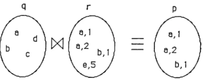
parallel execution of q and r may cause binding conflicts when they try to instantiate the shared variable X to two different values. When the clause p is called with unbound arguments, q( X) and r { X , Y ) may find different solutions for X . The result of p( X, Y) is the X values matching in q and r, plus Y values. So the value of p is obtained by joining sets which are formed by q( X) and r(X, Y) . Fig. 2.5 illustrates an example join operation.

It is impractical to allow parallel execution of each subgoal and then to check the consistency of all bindings obtained from each subgoal, and trying to find out all possible solutions for subgoals may cause the search space explosion problem [16]. So, some form of partial AND parallelism is more suitable.

Figure 2.6: Execution graph

There are two common approaches to handle partial AND parallelism :

• Stream AND parallelism • Restricted AND parallelism

Stream AND parallelism [6] [13] is a form of AND parallelism where subgoals communicate via shared variables. Referring back to the exam­ ple clause, subgoals q(X) and r(X,Y) could be executed concurrently where q is the producer and r is the consumer for X.

Restricted AND parallelism [12] [9] [13] refers to simultaneous evaluation of independent subgoals, i.e., subgoals that have no variables in common. It is called restricted because mutually dependent subgoals are still executed serially. For example, consider the following clause instance :

p{X, Y) : - r{ Xl qi X), s i Y) .

Since r and q share the variable X , one of them is dependent on the other one. Let r be the independent subgoal, and q be the dependent one. Then, r and s can staid simultaneously since s is also independent, while q is waiting for r. The order of execution can be shown by the execution graph in Fig. 2.6.

Selection of independent subgoals is performed by checking data depen­ dencies among the subgoals. This check can be done either at comi^ile-time

or run-time.

Trivial compile-time decisions may cause undesired situations since data dependencies are strictly related with unification. Checking dependencies and selecting independent subgoals at run-time [10] results in optimum par­ titioning. Below, compile-time and run-time dependency checking methods are compared :

Consider the following clause, p ( A ', y ) : - r ( A ') ,5( n

: - p ( T ,T ) .

Compile time inspection says that r and q can start in parallel since they are independent. In fact, during execution, the call p(T,T ) causes the variables X and Y to become aliases. Conse­ quently, r and q should be executed serially since the values for X and Y should match.

Now, consider the clause, p(A', V) : - r ( X , V), q(Y).

: - p ( A , a ) .

In this situation, compile time checking results in a set of depen­ dent subgoals (r, q) since they share the variable F , i.e, r and q will be executed serially.

But, at run-time, the call p( X, a) yields Y to be bound to the constant a and the clause p would look like

at that time. Since r and q becomes independent, they can run in parallel.

The reason why trivial compile-time decisions present certain undesirable situations is simply that all variables are considered unbound at compile­ time. However, after unification, some variables might be bound to some constants or other variables, and data dependencies change significantly. The disadvantage of run-time checking obviously is the extra processing overhead whenever an AND node is to be evaluated.

In Conery’s A N D /O R process model [9] , data dependencies axe checked dynamically. A method described by DeGroot [12] takes some of the run­ time decisions into compilation time. Some decisions will remain to be done during run-time, but the processing overhead is less.

2.5

Parallel Prolog Execution M odel P P E M

The Parallel Prolog execution model that has been emulated is defined by Aybayflj.

It supports full OR parallelism. The AND parallelism supported by the model is similar to restricted AND parallelism. The strategy is as follows :

Subgoals in a clause are partitioned into disjoint sets such that subgoals in every set have some shared variables,i.e., each set is related with different parts of the solution.The left most subgoal in a set is selected as the sender subgoal and sender of all sets axe executed in parallel,by activating sender-OR processes. Inside a set, execution is serial in order to prevent binding conflicts of shared variables.

Figure 2.7: Execution of two set of subgoals p ( X , Y ) : - s { X ) , q ( X ) , r { T ) , t ( X , T ) , y ( Y ) .

the subgoals are grouped into two sets, provided that X,T, are independent with Y :

(s, q, r, t) (tj)

which can start execution in parallel. The execution graph is in Fig. 2.7.

Although restricted AND parallelism causes loss of parallelism due to executing only independent subgoals in parallel, consistency check of solutions reported by each subgoal becomes manageable and efficient.

An AND process is responsible to start child OR processes for each sub­ goal, and combine the results. After completion of all subgoals, the resulting bindings are passed to the parent OR ¡process.

OR processes receive bindings from child AND processes and pass the answers to parent AND process as they come instead of gathering and sending all answers at once.

Unlike sequential Prolog, the result of a clause evaluation consists of all bindings that satisfy that clause. Since the model tries to find all solutions,

there is no backtracking.

In this study, an earlier version of the model has been considered. Re­ cently, some modifications have been made on the model, and a new version of the model shall appear soon [3].

2.6

Parallel Architectures

Parallelism in Prolog can be realized only by implementing proposed par­ allel execution algorithms on parallel or distributed systems. In terms of efficiency, the key point is the matching between the parallel architecture and the parallel execution model. An execution model may not work as efficiently as expected on a particular architecture. Algorithms and the ar­ chitecture should talce into consideration their features to exploit maximum parallelism.

Granularity and communication requirements of the execution model are the prominent factors affecting the selection of the architecture, or vice versa, execution model should be modified according to the parallel architecture.

Granularity means the degree of parallelism [26]. Too much parallelism may cause a degradation in performance because of overwhelming the system with communication overhead, or too coarse-grain parallelism may not exploit potential parallelism.

There axe various parallel structures proposed so far. Parallel systems can generally be divided into three groups [15] :

• Array Processors, • Multiprocessors, • Data Flow Machines

Figure 2.8: Tightly coupled multiprocessor system

2.6.1

Array Processors

In array processors, multiple function units perform the same operation on different data [24]. Such array processors are suitable to a class of very structured problems, usuallj'· involving array types. They are efficient at data- parallel rather than task parallel problems. In [17], a parallel Prolog execution model, called DAP Prolog, is described running on an array processor.

2.6.2

Multiprocessors

Multiprocessor [15] [22] systems are composed of several processing elements, PE, and memories connected through an interconnection network. They can be divided into two categories :

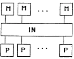
• tightly coupled systems where PE’s are connected through shared com­ mon memories, Fig. 2.8.

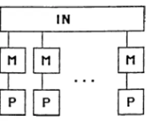
• loosely coupled systems where PE’s are connected through message links. Fig. 2.9.

In tightly coupled s3’’stems, fast communication between PE ’s is an ad­ vantage, but for large number of PE’s, performance decreases due to memory access contention.

Figure 2.9: Loosely coupled multiprocessor system

In loosely coupled systems, there is no shared memory. PE ’s can com­ municate via message exchange. So, design and topology of internetwork is vital for the performance of the system. Generally, communication is slower in loosely coupled systems than that of tightly coupled systems. Therefore, in loosely coupled systems, large granularity applications tend to be more effective compared with tightly coupled ones.

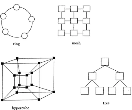
There axe different interconnection topologies proposed for the loosely coupled systems including ring, mesh, hypercube, and tree. Fig. 2.10 shows those topologies. In loosely coupled sj''stems, parallel algorithms should fit the interconnection topology since communication overhead might degrade the performance significantly [22].

In distributed systems, where PE’s are connected through relatively slower networks (local area networks, etc), fine-grain parallelism does not work effi­ ciently since communication takes considerable time compared with process­ ing time.

There are various implementations of parallel Prolog on multiprocessor architectures. They include Aquarius project [4] [28], Shapiro’s Flat Concur­ rent Prolog [25].

mesh

tree hypercube

Figure 2.10: Interconnection topologies

2.6.3

Data Flow Machines

Data Flow computers are really a radical departure from Von Neumann com­ puters [11]. In a Data Flow computer, there is no notion of program counter. An instruction is ready for execution when its operands arrive. Parallelism is in the instruction level, that is, very fine grain parallelism is achieved compared to the array or multiple processor systems. One major problem with Data Flow computers as well as other highly parallel machines is that concurrency is limited Iw the communication network [15]. A parallel Pro­ log execution model suitable for Data Flow computers is proposed in [14],by Hasegawa and Amamiya.

3. Implementing A N D /O R Parallelism

3.1

A N D /O R Process

A node of an A N D /O R tree corresponding to a Prolog program represents a single activity. A process is defined as a discrete unit of computer activity, and a node or a collection of AND nodes form a process. That means, granularity of a process cannot be finer than an A N D /O R node, and can not be coarser than a procedure (i.e, all descendant AND nodes of an OR node) as shown in Fig. 3.1

The meaning of grouping AND nodes as a single process is that the AND nodes are to be solved serially in that group. The purpose of grouping is to play with the granularity of the model.

Processes can communicate with each other through their interfaces, but in the execution model ¡Drocesses need to communicate with only their parents or immediate descendants. Internal working of a process is hidden from the other processes.

To give a better explanation of execution, consider the following program:

p { X , Y ) : - r { X ) , q { Y ) . p(a, b).

a) AND nodes are evaluated in parallel

b) AND nodes are evaluated serially

Figure 3.1: AN D /O R processes r(c).

q(b).

: -p (b , T).

When a clause instance is to be evaluated, -AND process-, the terms in the clause head are unified with the list that is sent by the parent process which is called unilist.

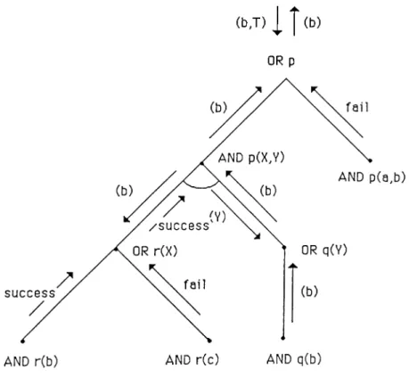
If unification succeeds and there are subgoals, the AND process creates an OR process for each independent sul^goal and prepares their unilists. Then OR processes continue by creating AND processes for the candidate clauses in the procedure. The goal of the example with the A N D /O R tree repre­ sentation illustrated in Fig. 3.2, is p(a,T). An OR process is created for procedure p, and that OR process looks for clauses with clause head p, i.e candidate clauses in the procedure. Then it creates AND processes for each p clause. Next, AND-p(A^, Y) and AND-p(a, b) try to match the unilist and their term-list. The first AND process bounds X to b and Y remains non­ ground, while the second one fails to unify and immediately sends a failure message to its parent. The former one continues by creating OR processes

(b J ) 1 1 (b)

OR p

Figure 3.2: A N D /O R tree representation of the example

for subgoals r and q and waits for the messages from their descendants.

The purpose of this example is to explain the execution briefly. All details of the execution, and the process communication will be discussed in the next chapter.

3.2

A N D Parallelism

As described in the execution model, a form of restricted AND parallelism is supported and subgoals in a clause are partitioned into disjoint sets called C Ji CLUTfS ·

A chain is a collection of subgoals that are either directly or indirectly dependent on each other. Chains can be found by drawing an undirected graph where vertices are subgoals and edges are the shared variables. Each

q(T)

t(Q)

s(W)

W

v(Z,W)

Figure 3.3: Graph for the chains

connected component of the graph corresponds to a chain. In Fig. 3.3, a graph for the rule

p{X, Y, PF, Q) : - r ( X , Y), q{T\ s(PF), t{Q), u(T, F ), v(Z, W )

is constructed. The connected components of the graph represent the chains

(r,q,u)

(t)

Chains are computed at run-time, as described in Chapter 2. Data depen­ dencies are checked after the unification operation is performed. So different instances of a clause may have different chains.

3.2.1

Execution of a Chain

Each chain is evaluated independently, and inside a chain execution is serial. After all chains are comjDleted, liindings formed by each chain are combined to form the solution set of the clause.

Figure 3.4: Execution of a chain

The first subgoal in a chain is started as a sender OR process. When bindings come from the sender, next clause in the chain is started as a receiver OR process. The order of subgoals execution in a chain is left-to-right.

For each tuple produced by the sender, receiver process gets values of shared valuables, and tries to find all solutions. After processing all the tuples produced by the sender, the AND process combines, (equijoin) , bindings set of the sender and the receiver processes to Ido used by the next receiver, if any.

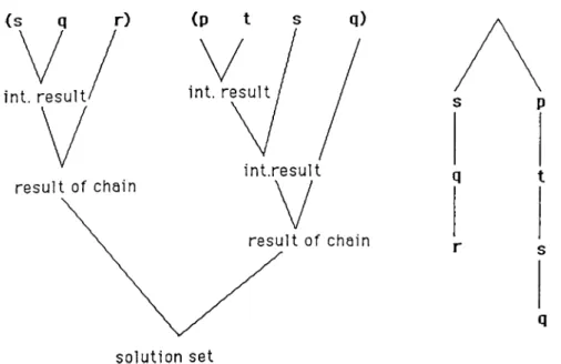
At the end, the last receiver process completes its function and the resulting set is the bindings of that chain. Fig. 3.4 illustrates execution of a sample chain. The result of all chains are combined by taking Cartesian product of them since partitioning guarantees that there exists no shared data between chains.

Figure 3.5: The set S and 1Z

3.2.2

Join Operation

Join and Cartesian product operations may take considerable time in AND processes, so efficient methods should be developed to increase the perfor­ mance. When a receiver process completes its function, previous set of bind­ ings and the result of the receiver process should be combined by joining the results.

What makes the implementation of join operation more difficult them that of a normal join operation as in relational data bases is the fact that values of the columns may contain unbound variables, structures with variables and variables bound to another unbound variable. Prolog variables are quite different from the variables of conventional computer languages. Unification of two unbound variables in effect links them, so that if one variable receives a value, the other has exactly the same value.

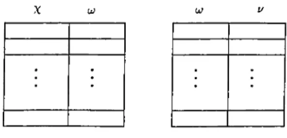
Let <5 be a set of tuples already constructed by a process Ps, and Pn be a receiver process which produces the set TZ. Further, let tuples of S have the attributes x, , tuples of P have the attributes a;, u where x , u) and i/ are set of unique variables and u is shared between S and TZ. In other words X n = 0 as shown in Fig. 3.5

For each tuple in «S’, Pr gets values of u from the set S and returns possibly

Figure 3.6: Bindings when i/ = 0

a set of bindings. Depending on u; and u, what Pfi returns is discussed below :

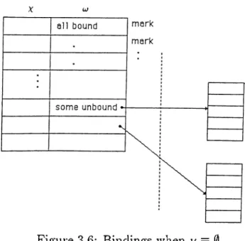
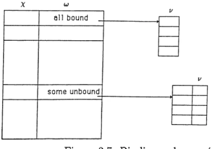
• TZ has no unshared variables, i.e,u = 0

if value of u> in tuple of S, Su,(i) has no unbound variable then Pn only checks the truth of 7^(w) and marks Su,{i) either valid or invalid depending on the result.

If (jj contains some unbound variables then Pp, possibly returns a set of bindings for those unbound variables, and marks valid pointing to the bindings, or if Pp fails then Su,(i) is mai'ked as invalid. Fig. 3.6 illustrates this situation.

• P contains some unshared variables, i.e^u ^ 0

Similar to the previous case, Pp gets values of u from and returns bindings for 1/, and depending on oj, bindings for u) as illustrated in Fig. 3.7

• TZ has no shared variables, i.e,a; = 0

Although it seems strange that the receiver process and the sender process has no common variables, it may happen due to the definition of the chain. Consider the following example,

Figure 3.7: Bindings when u ^ ^ where the graph representation is

X T

p ---r

---p, q, r are related with each other, so ---p, q and r form a chain. Since the order of execution is left-to-right the subgoals are evaluated in the order they are written, p, q and r where p and q has no variables in common.

In this case, Pr is executed once, not for all tuples in S, and instead of joining the results, Cartesian product of them is sufficient.

After Pr processes every tuple in S, it is enough to substitute values from

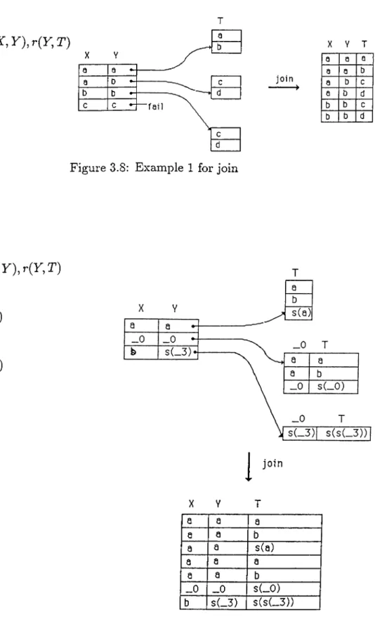
7^ in <5 in order to combine results. In Fig. 3.8 and 3.9, two examples of the join operation axe illustrated. The second one is more complex since u contains variables rmd a structure with variables.

3.2.3

Duplicate Bindings

In Fig. 3.8, the receiver process Pr computes the set (c, d) two times because

in the column u there are two 6’s. In other words, duplicate values in uj causes unnecessary computations.

Even if the tuples are unique in the set S, projection over u> may contain duplicate values. In order to increase performance, unnecessary executions of Pr should be eliminated. The method that is used is :

....p {X ,Y ),r {Y ,T ) p(a, a) p(a, b) p(b, b) p(c, c) r(a, a) r(a, b) r(b, c) r(b, c) a a a D -b b -c c b X Y T a a a a a b c j o i n a b c d a b d b b c b b d

Figure 3.S: Example 1 for join

...p(X,V),r(r,T) p(a, a) p ( X , X ) p (b ,s(X )) r(a, a) r(a, b) r ( X , s ( X )

1

Figure 3.9: Example 2 for join

Figure 3.10: Duplicate values in a set

_0 a(_0,_l)

_0 a ( - F - 2 )

_0 a(_1,_I)

Figure 3.11: Duplicate columns containing structures with variables When Pr is completed for tuple all tuples that have the

same values in u column as S^{i) are marked as if they are pro­ cessed. The next tuple to be used by the Pr is the first unmarked tuple after the current one. This method is illustrated in Fig. 3.10 In the figure, , Su{3) and <Fc^(4) axe duplicates and they point to the same solution set.

Duplicate checking becomes more complex if uj contains structures with

variables. Consider the set in Fig. 3.11 Although it seems that a(_0, _1), a(_l, _2) are different, from Pr'spoint of view, they are the same. In other words, Pr

computes the same bindings for both structures. The problem is how the sets are joined. The solution is to establish the mapping between variables. In this example, the variables _0, _1 in the first structure are associated with the variables _1,_2 in the second one. This mapping is used when substituting

p(X ,a(X ,Y ))

p(X,a(Y,T))

p(X,a(Y,Y))

Figure 3.12: Joining duplicate structures

values found by Pr during the join operation. In figure 3.12 this method is

shown. Note that substituting the same set in the first two tuples results in completely different tuples.

3.2.4

Cartesian Product

After all chains are completed, the bindings formed by each chain should be combined to construct the final binding set , or the solution set of the clause. Since partitioning the subgoals guarantees that the bindings set of chains have no variables in common, those sets are combined by the Cartesian

product operation. In order to get the solution set, it is necessary to project the output of the Cartesian product operation over the variables requested by the caller clause.

Solutionset = n(xf=iC ,·)

where C,· denotes the binding set of chain i. Projection operation, repre­ sented by n is taken over the variable set required by the parent process.

Let

p (a ,A ',y ) : - r ( X U ( T , Y l 4 Y ) , t ( Z ) M Z )

be an instance of the clause p, and values of X and Y be the set of variables requested by the parent process. For this instance of p, the following clause sets are the chains ;

(r)

(i,u )

and the bindings set for each chain has the attributes :

Cl S {X }

C2 s {T ,Y ]

C3 = {Z }

After applying the Cartesian product,

Cl X T Y

z

IIxC,· (after removing

duplicates)

Figure 3.13: Cartesian product operation

is the set of variables in the result. Since only the X and Y values are required to pass to the parent, the set {A', T, F, Z } is projected over X , Y resulting in

In Fig. 3.13, the above operations are illustrated with sample sets.

Some improvements related to both storage and time can be done in Cartesian product and projection operations.

Instead of taking Cartesian product first, projection can be performed on bindings set of each chain, then resulting sets are combined by taking cartesian product.

Solution set = XiLidJC,·)

This method uses less storage and time, since redundant attributes are eliminated before taking the Cartesian product operation. Referring back to the previous example,

riA'y(<^i) = riA’'K(^2) = { y }

= 0 xf=l(riA'y(<^l)) =

Projection operation takes no extra memory or computation time like Cartesian product, because it is sufficient only to find out which columns of the binding sets are in projection variable set.

If the second method is applied for the example in Fig. 3.13, output of the Cartesian product would be directly the same as the solution set, and no storage would be used to store the tuple values {X , Y", T, Z } which is computed in Fig. 3.13.

3.3

O R Parallelism

3.3.1

Pipelining

An OR process, as its name implies, creates one or more AND processes for alternative solutions. Bindings from AND processes may arrive at OR processes asynchronouslj^ In the execution model, an OR process does not wait for all solutions to combine and send them at once. Instead of gathering the bindings, it just passes bindings as they come, so that the parent AND process can process the data immediately. This strategy is called pipelining. But, use of pipelining is limited to only sender processes, i.e, intermediate results coming from OR processes can be used only by the fii'st receiver

AND AND

b) Figure 3.14; Or pipelining

process. To be more explicit, consider the following case :

Let (s, q, r) be a chain. Execution starts by creating a sender OR process for subgoal s while r and q is waiting, as in Fig. 3.14(a).

As intermediate results come from the sender process, the subgoal q can be evaluated simultaneously using bindings so far produced by s. Fig. 3.14(b).

However the subgoal r can not be started even if some intermediate results come from the subgoal q, because it has to wait for the result of the join operation.

3.3.2

Some improvements in O R processes

Execution of an OR process can be controlled more intelligently by taking some properties of the clauses into consideration.

One improvement is related with OR processes where the unilist sent by the parent process has no variable in it. In this case, OR process does not return any bindings because the unilist is composed of constant terms. Instead, it sends a SUCCESS or FAIL message to the parent AND process.

with a call p(a, Y ) resulting in X to be bound to constant a. For this situ­ ation, it is sufficient to know whether r(a) is true or false. So at least one success message from the OR process which is created to solve the subgoal r is enough for the AND process. Consequently, the process OR-r can ter­ minate as soon as finding one successful result without waiting for the other alternative solutions.

Another similar improvement, which may not be practical but might be interesting from a theoretical point of view is explained below :

p(X,Y) : -q(T),r(X,Y)·

p(A',

Y)

:

-r(X ), q(Y)

with a call p { X , Y ) . Contrary to the first case, in this clause, the unilist contains one variable for the subgoal q, and normally the process OR-5 will return a set of bindings. However the complete set is not needed to evaluate the conjunction of subgoals because the variable T is not involved neither in the clause head nor in the subgoals. Like the previous case, only one binding for T is enough for the evaluation of the clause. If the relation q has a large solution set, it might be beneficial to detect such cases.

4. ST R U C T U R E OF THE E M U L A T O R

4.1

Parallel Prolog Emulator

The emulator program is written in C programming language running on Unix 4.2BSD on a SUN 3/160 workstation. The emulator itself runs on a uniprocessor system, so it is in fact a combination of Parallel Prolog emulator on top of a multiprocessor simulator.

The emulator is developed using discrete-event simulation technique with an object oriented approach [21].

Object oriented style is imitated as much as possible, although C makes this difficult to achieve. In object oriented approach, operations are clustered around objects which are modules representing a closure of information and all actions that are allowed to access/change this information. Objects receive and react to messages through their interfaces [21].

In C, classes of objects can be represented by structure types, and meth­ ods are the functions manipulating objects. Instances of objects are created at run-time by using dynamic memory cillocation. Since object types and modules cannot be clustered into a single textual module in C, object names are passed as a parameter to functions that manipulate them.

In the emulator, there exists one object class only which is called process and it is defined as a structure type.

Figure 4.1: Parallel Prolog Emulator

4.2

System Parameters

Emulator reads two input files, parameters and a Prolog program, at the beginning to set up the environment as shown in Fig. 4.1. System parameters file contains specifications about the machine and the timing information. Execution time of operations are given in terms of unit-time. Elapsed time for an operation is expressed relative to other operations. For example, process creation may teike 20 time units, while process switch takes 5 time units. It is not important what real time a time unit corresponds.lt might be one second or one millisecond.

The parameter file contains the following information :

n u m ofp rocessors Number of processing elements in the system,

em u la tion -tim e Maximum allowed emulation time,

p et Process creation time,

pst Process switching time.

sralgt Sender-Receiver run-time selection overhead,

jo in b a se Join operation base time,

ca rtb a se Cartesian Product operation base time,

m arkbase Duplicate check base time, d u p ch eck Duplicate check flag.

4.3

Timing

Process-creation, process-switching, uniflcation, join, cartesian product, and duplicate check operations are considered as time consuming activities. In order to compute the execution time of a particular activity, the function

getelaptime{count, operation-type)

is called. This routine returns how many time units a speciflc operation takes.

Time units calculated for an activity is a function of the parameter count and the base-time (i.e., elapsed-time = /(count,base-time)) of that operation which is specifled in the parameters file. The variable count has the following meaning :

for un ification Number of simple term unifications,

fo r jo in Size of the result in terms of constant data type, for cartesian Size of the result in terms of constant data type,

fo r d u p lica te check Number of tuples searched.

Currently, the function getelaptime takes the sum of count and base-time (i.e., elapsed-time = count + base-time), to calculate the execution time of an operation, because thei’e is no study done yet about the timing estimations of

those operations. In order to obtain better estimates of timing getelaptime could be modified.

4.4

Performance Measures

In the emulator, the following performance indexes are measured :

For each Processor Element : • utilization of the processor, • average ready queue length, • average waitq queue length, • number of processes,

• percentage time for process creation , • percentage time for process switching , • percentage time for unification operations, • percentage time for join operations,

• percentage time for Cartesian product operations, • percentage time for duplicate check operations. System wide measures include :

• average system utilization, • number of total processes, • Prolog program execution time.

4.5

M odel of the Architecture

A multiprocessor system is simulated by modelling such that it supplies suf­ ficient facilities for processs creation, execution, and communication. The

Figure 4.2: State diagram for FCFS

reason for this is that we are mainly interested in the behaviour of the ex­ ecution model on the architecture. Performance of the execution model is measured in terms of some basic parameters of the system.

One assumption is that each Processing Element can access the shared common memory without any memory contention. It is not a very unrealistic assumption because high memory bandwidth can be achieved by employing a proper, fast interconnection network in addition to cache memories. Memory contention leads certainly a decrease in performance of the total system by some percent, but it does not dei^end on the execution model significantly, because in the execution model each process sends a copy of unilist to its immediate descendants instead of sharing them. So each process works on its own local data and memorj'· access problems are unlikely to occur.

Communication between processes is achieved by message exchange. Since the architecture is tightly coupled, communication takes place very fast com­ pared to loosely coupled ones by just passing a pointer to the message , not the message itself.

Each Processor in the system can execute processes concurrently. Pro­ cessor management policy is selected to be First-Come-First-Served (FCFS). The processes created by the execution model do not keep the processor busy

for a long time. The operations that need computation are unification and set operations.

A process that is in running state becomes blocked when it finishes its current function and waits for a message to continue. When a blocked process receives a message, then it becomes ready to be executed and it enters the ready queue.Fig. 4.2 illustrates those states. As a processor becomes idle, the first process in the ready queue grasp the processor.

4.6

Intermediate Code

Prolog programs to be emulated are written in an intermediate code format [27]. The intermediate code consists of the following primitives :

$get < te r m list> list of terms in a clause head $put < te r m list> list of terms in a subgoal

$ or < s u b g o a l> corresponds to a subgoal in the clause body $p_c turns on AND parallelism

$s_c turns off AND parallelism Sreturn terminates a clause

Send specifies end of intermediate code

{ , } blocking operators to combine two or more alternative clauses in a pro­ cedure

4.6.1

Translation from Prolog to Intermediate code

is translated into intermediate code as follows

%Q€-i , 5 t/f

% P -C

$put Ui,. . . ,Un

$or qi

$put Vi,. . V,n

$or qi

treturn

Similarly translation of a fact

results in :

p{tx,...,tk).

%qd j ) ik

%return

The goal clause

is converted as : goal-fit f X) ·. · ^ tk tor p treturn : - p(ti,...,tk).

An intermediate code program is a collection of the above transformations with the following restrictions :

• All alternative clauses that form a procedure should be grouped to­ gether, i.e, they should follow each other .

• Beginning of a procedure is specified by appending an underscore char­ acter to the end of the first clause name in that procedure.

• Goal clause should be at the beginning.

The following example is a Prolog program and its conversion into the intermediate code. Prolog program : p (X , a, h(Y, Z)) : - r ( b ( X , c(d)), s(Y, b(Z)). p(a, b ,X ). p(a,a,b). r{b(a, r ) ) . s(a, b{a)). :

-p(X,a,Z).

Corresponding intermediate code: goal-$get X , a, Z $or p ^return

$return $get a, b, X %return P %get a, a, h %return r. $get b{a, Y ) $return s. $get a, b(a) treturn %end

4.6.2

Built-in Functions

In order to perform arithmetic and relational operations, some built in func­ tions are provided. These functions are :

ADD(N1,N2,N3) : Nl = N2 + N3

SUB(N1,N2,N3) : N 1 ^ N 2 - N 3

MUL(N1,N2,N3) ; N1 = N2 * N3

DIV(N1,N2,N3) : N1 = N2/N3

EQU(N1,N2) : iVl = = N2

NEQ(N1,N2) : -VI

N2

L E Q (N 1,N 2) : 7V1 < A^2

L E T (N 1,N 2 ) : iVl < N2

G E Q (N 1 ,N 2) : N1 > N2

G R T (N 1 ,N 2) : N l > N 2

In order to carry out the operations, right-hand side of arithmetic oper­ ators, and both side of relational operators should be integer constants or ground variables, i.e, those functions can be invoked by passing constant or ground variables. For this reason, the order of built-in functions in the clause body is important. For example, in the following clause :

p ( X , i V l ) ; - q { X ,N 2 ,N Z \ A D D { N l ,N 2 ,N Z ) .

the subgoal q is supposed to bind some integer constant values to variables N2, and NZ. It will be incorrect if the order of q and A D D is exchanged, because the emulator will try to evaluate the function A D D before «¡r, since A D D and q forms a chain.

4.6.3

Playing with Granularity

Blocking operators provide us to play with the level of parallelism in addition to the primitive $s_c which turns off the AND parallelism. If some clauses in a procedure are required to be executed serially, those clauses are blocked by using the operators { and }. That restricts the OR-parallelism, in other words OR process creates one process to evaluate a block of clauses which is illustrated in Fig. 4.3.

If the program is to be executed sequentially , then all procedures are blocked and $s_c is used to prevent AND parallelism.

OR p

(AND p (x i^ ■ AND p(a), AND p(5T'^

' — :--- '

Figure 4.3: Blocking clauses in a procedure

4.7

Data structures for bindings

The key point in developing a program is to construct a suitable data struc­ ture to represent the algorithm better. This section and the next one discusses data structures used in the emulator.

4.7.1

Representation of terms

If possibility of forming a cyclic structure is ignored, all terms can be repre­ sented by directed acyclic graphs [5]. Cyclic structures may be created during unification. For example, if the terms f ( x ) and x are tried to be unified, it will result in an cyclic structure:

/ ( / ( / ( / · · ·

Such cases should be eliminated while writing Prolog programs.

Fig. 4.4 shows the representation of terms

a) Before unification

b) After unification

Figure 4.5: DAG representation of terms with offsets

In the implementation , variable nodes are offsets to local variables table of the clause. In that case , the example in Fig. 4.4 takes the form as in Fig.. 4.5.

4.7.2

Basic Data Types

Basic data types supported by the emulator are

• constants,

• integer constants,

• variables,

• structures.

To represent those data types, a two-field data structure is used , and its form is shown in Fig. 4.6

Status Term

Figure 4.6: The structure for a simple term T E R M indicates whether it is a term or member of a structure, L A S T T indicates that it is the last element of a structure,

C O N constant data type , term field points to the constant value, V A R variable, term field is an offset to local variable table,

S T R U C T structure, term field points to the symbol which is the functor. I N T integer constant, term field itself contains the value, (valid if CON is

also specified )

In Fig. 4.7 representation o f the terms :

X J ( a , X , b ( 2 , Y ) ) , a

is illustrated.

In Fig. 4.8, the terms t( X ,q (Y )) and t{p (Z ),V ) whose DAG representa­ tion is shown in Fig. 4.4, is shown by using the data structure discussed.

Standard Prolog also supports the list data type which is widely used in non-numeric programming. A list is a sequence of any number of items. A list can be written in Prolog as :

[a, 6, c, d, e]

The first item in the list is called the head of the list, remaining part of the list is called the tail. In the previous list, the head is the symbol a, and

Local variable table___ X:0 Y:1 TERM,VAR _0 TERM,STRUCT CON VAR _0 LASTT,STRUCT C0N,INT 2 LASTT,VAR _ I TERM,CON f a

t

Figure 4.7: Representation of a term-list

X:0 Y:1 Z:2 V:3 free free TERM.STRUCT VAR _ 0 ,^LASTT,STRUCT LASTT,VAR _1 TERM,STRUCT STRUCT LASTT,VAR _2 LASTT,VAR _3

7

.(a, .(b, .(.(c, .(cl, .(e, ml))), ml)))

Figure 4.9: Representation of lists

the tail is the list [6, c, d, e]. In Prolog, head and tail of a list is expressed as :

[H ead\Tail]

thus, an alternative way of writing above list is [a|[6, c, d, e]].

In the emulator, although lists in that format is not supported directly, a list in the form [iTead|Taz7]can be written as :

.(Head, Tail)

and a single element list [a] can be written as :

.(a, nil)

In fact this notation [5] is the internal representation of the lists. In Fig. 4.9, representation of the list [a, b, [c, d, e]] is illustrated.

status term r Number of elements { EOLIST Number of elements Number of distinct variables

Figure 4.10: Structure of unilist and glist

4.7.3

Data structures for Unilist and Uniresult

unilist and uniresult are the two important data structures used in the unifi­ cation. The unilist is the list of terms that is sent by the caller side, and it is unified with the terms in the head of the called clause which is referred as glist by using unification rules described in [2]. Fig. 4.10 shows the structure of unilist and glist.

Consider the following clause

v i X , Y , a ) : - r { X , Y )

with a call p(b,T,a). Then, unification environment of that call instance would be as illustrated in Fig. 4.11.

When the evaluation of the clause is completed, bindings to uninstantiated variables in the unilist are reported back by constructing the data structure uniresult. The uniresult data structure is composed of tuples where size of the tuple is equal to the number of distinct unbound variables in the unilist. There might be more than one tuple, since all bindings satisfying the clause are found. Fig. 4.12 shows the structure of the uniresult.

Local variable table 0

1

Figure 4.11: Unification environment for a particular instance

status term

size of list

size of list number of tuples

4.7.4

Bindings containing unbound variables

As described before, each variable is an offset to local variable table of a clause instance. Each instance of a clause has a private local variable table. T hat m eans, variables valid in the scope of the clauses and variables in different instances having the same offset values are absolutely irrelevant.

However, bindings containing unbound variables present an im portant problem related w ith variables. For example, consider the following case :

p ( x , Y ) ■.- r ( Y U ( x ) ·

т(ЫТ, V)).

Variables AT, Y have offsets 0 and 1 in clause p, and also T, V have the offsets 0 and 1 in clause r. W hen r is invoked by p, it returns the bindings 6(_0,-1) where .0 and _1 represent variables. W hen this result is received by p, variable num bers conflict because _0 and _1 corresponds to A , Y whereas in result 6(-0, _1) variables _0 and _1 are completely different variables. So a way should be found to differentiate those variables in bindings set from the local ones.

The solution which is used in the the em ulator is as follows :

Local variable table of a clause consists of two logical p arts , one p a rt is the locations reserved for variables in the unilist, the other p a rt is the variables in the clause. It is illustrated in Fig. 4.13. Furtherm ore, when a clause is invoked, the unilist for th a t clause is prepared such th a t variables in the unilist is ordered starting from offset 0 to m where m is the num ber of distinct variables in the unilist. Since variables in the original unilist may not be con­ tinuous , a m apping is kept to recover the variables after ordering

locations reserved for variables in uni list. ■\ locations reserved ¡> for variables in the clause

J

Figure 4.13: Local variable table

1 1 ₁ 1 VAR _5 VAR . 0 VAR _7 VAR _ 1 VAR _5 VAR . - . 0 VAR VAR _2 1 .. 1 1 with mapping 0 — ► 5 1 - + 7 2 — > 0

Figure 4.14: Ordering the variables

them . Fig. 4.14 shows this situation clearly. W hen the uniresult is received, if an unbound variable offset is between 0 and m, th a t m eans it belongs to the caller clause. If it is greater th an m, it is not a local variable, so its offset is adjusted as being greater th an the size of the local variable table.

4.8

System Related Data Structures

Before startin g the em ulation, interm ediate code is further converted into an object code to make the interpretation easy, and it is p u t into an area called

4.8.1

Clause table

For each clause definition, an entry is reserved in a table called clausetable. An entry has the following fields :

n u m a t N um ber of subgoals in th a t clause,

n u m v a r N um ber of distinct variables in th a t clause,

a iid fla g If andflag is true, AND parallelism for th a t clause is tu rn ed on, g lis t List of term s in the head of the clause,

p lis t Array of list of tei'ins for the subgoals in th a t clause.

The d a ta stored in the clausetable is static, i.e, it does not change during execution. W henever an AND process is created to evaluate a clause, the process copies the tem plates from the clausetable to its local environment to perform the unification and other operations, because there may be many instances of the same clause with the different set of d a ta in the system.

4.8.2

Process Representation

As stated before, a process is represented by a d a ta stru ctu re as illustrated in Fig. 4.15.

The function of the fields in the process stru ctu re is as follows:

e v e n ttim e If the process is scheduled for an action, the completion tim e is recorded in eventtime.

p s t a t It specifies the type of a process. It may be a INIT, OR, or AND process. If it is an OR process, p sta t indicates also w hether the process