Selçuk J. Appl. Math. Selçuk Journal of Vol. 11. No.1. pp. 3-13 , 2010 Applied Mathematics
Homotopy Perturbation Method for Solving a Three-Species Food Chain Model
Mehmet Merdan
Civil Engineering, Engineering Faculty, Gümü¸shane University, Gümü¸shane, Türkiye e-mail: m erdan29@ hotm ail.com
Received Date: January 31, 2008 Accepted Date: November 24, 2009
Abstract. In this article, homotopy perturbation method is implemented to give approximate and analytical solutions of nonlinear ordinary di¤erential equa-tion systems such as a three-species food chain model. The proposed scheme is based on homotopy perturbation method (HPM), Laplace transform and Padé approximants. Some plots are presented to show the reliability and simplicity of the methods.
Key words: Padé approximations; Homotopy perturbation method; a three-species food chain model.
2000 Mathematics Subject Classi…cation: 34A34; 34A35. 1.Introduction
Dynamics of chaotic dynamical systems as a three-species food chain model is ex-amined at the study [1]. The components of the basic tree-component model are proportional to the population density of the lowest trophic level species (prey), the middle trophic level species (intermediate predator) and highest trophic level species (top predator)is denoted respectively by x(t); y(t) and z(t) These quantities satisfy (1.1) 8 < : dx dt = x(a1 b1x c1y) dy dt = y( a2+ c2x d1z) dz dt = z( a3+ d2y)
with the initial conditions:
Throughout this paper, we set a1 = 4; a2 = 0:3; a3 = 0:15; b1 = 0:01; c1 =
14; c2= 0:3; d1= 0:1; d2= 0:05:
The motivation of this paper is to extend the application of the analytic homotopy-perturbation method (HPM) to solve the a three-species food chain model (1.1). The homotopy perturbation method (HPM) was …rst proposed by Chi-nese mathematician He [9–13,16-17,20]. The …rst connection between series solution methods such as an Adomian decomposition method[3-8] and Padé approximants was established in [14, 15].
2 Padé approximaton
A rational approximation to f (x) on [a; b] is the quotient of two polynomials PN(x) and QM(x) of degrees N and M, respectively. We use the notation
RN;M(x) to denote this quotient. The RN;M(x) Padé approximations to a
function f (x) are given by [21]
(2.1) RN;M(x) =
PN(x)
QM(x)
for a x b
The method of Padé requires that f (x) and its derivative be continuous at x = 0. The polynomials used in (2.1) are
(2.2) PN(x) = p0+ p1x + p2x2+ ::: + pNxN
(2.3) QM(x) = 1 + q1x + q2x2+ ::: + qMxM
The polynomials in (2.2) and (2.3) are constructed so that f (x) and RN;M(x)
agree at x = 0 and their derivatives up to N + M agree at x = 0. In the case Q0(x) = 1, the approximation is just the Maclaurin expansion for f (x). For a
…xed value of N + M the error is smallest when PN(x) and QM(x) have the
same degree or when PN(x) has degree one higher thenQM(x).
Notice that the constant coe¢ cient of QM is q0 = 1. This is permissible,
because it notice be 0 and RN;M(x) is not changed when both PN(x) and QM(x)
are divided by the same constant. Hence the rational function RN;M(x) has
N + M + 1 unknown coe¢ cients. Assume that f (x) is analytic and has the Maclaurin expansion
(2.4) f (x) = a0+ a1x + a2x2+ ::: + akxk+ :::;
And from the di¤erence f (x)QM(x) PN(x) = Z(x) :
(2.5) "1 X i=0 aixi # "M X i=0 qixi # "N X i=0 pixi # = " 1 X i=N +M +1 cixi # ;
The lower index j = N + M + 1 in the summation on the right side of (2.5) is chosen because the …rst N + M derivatives of f (x) and RN;M(x) are to agree
at x = 0.
When the left side of (2.5) is multiplied out and the coe¢ cients of the powers of xi are set equal to zero for k = 0; 1; 2; :::; N + M , the result is a system of
N + M + 1 linear equations: (2.6) a0 p0= 0 q1a0+ a1 p1= 0 q2a0+ q1a1+ a2 p2= 0 q3a0+ q2a1+ q1a2+ a3 p3= 0 qMaN M+ qM 1aN M +1+ aN pN = 0 and (2.7) qMaN M +1+ qM 1aN M +2+ ::: + q1aN + aN +2= 0 qMaN M +2+ qM 1aN M +3+ ::: + q1aN +1+ aN +2= 0 qMaN + qM 1aN +1+ ::: + q1aN +M +1+ aN +M = 0
Notice that in each equation the sum of the subscripts on the factors of each product is the same, and this sum increases consecutively from 0 to N + M . The M equations in (2.7) involve only the unknowns q1; q2; q3; :::; qM and
must be solved …rst. Then the equations in (2.6) are used successively to …nd p1; p2; p3; :::; pN[21].
3. Homotopy perturbation method
To illustrate the homotopy perturbation method (HPM) for solving non-linear di¤erential equations, He [18, 19] considered the following non-linear di¤erential equation:
(3.1) A(u) = f (r); r 2
subject to the boundary condition
(3.2) B u;@u
@n = 0; r 2
where A is a general di¤erential operator, B is a boundary operator, f(r) is a known analytic function, is the boundary of the domain and @n@ denotes di¤erentiation along the normal vector drawn outwards from . The operator
A can generally be divided into two parts M and N. Therefore, (3.1) can be rewritten as follows:
(3.3) M (u) + N (u) = f (r); r 2
He [19,20] constructed a homotopy v(r; p) : x [0; 1] ! < which satis…es
(3.4) H(v; p) = (1 p) [M (v) M (u0)] + p [A(v) f (r)] = 0;
which is equivalent to
(3.5) H(v; p) = M (v) M (u0) + pM (v0) + p [N (v) f (r)] = 0;
where p 2 [0; 1] is an embedding parameter, and u0is an initial approximation
of (3.1). Obviously, we have
(3.6) H(v; 0) = M (v) M (u0) = 0; H(v; 1) = A(v) f (r) = 0:
The changing process of p from zero to unity is just that of H(v,p) from M (v) M (v0) to A(v) f (r). In topology, this is called deformation and M (v) M (v0)
and A(v) f (r) are called homotopic. According to the homotopy perturbation method, the parameter p is used as a small parameter, and the solution of Eq. (3.4) can be expressed as a series in p in the
form
(3.7) v = v0+ pv1+ p2v2+ p3v3+ :::
When p ! 1, Eq. (3.4) corresponds to the original one, Eqs. (3.3) and (3.7) become the approximate solution of Eq. (3.3), i.e.,
(3.8) u = lim
p!1v = v0+ v1+ v2+ v3+ :::
4. Applications
In this section, we will apply the homotopy perturbation method to nonlinear ordinary di¤erential systems (1.1).
4.1 Homotopy perturbation method to a three-species food chain model
According to homotopy perturbation method, we derive a correct functional as follows:
(4.1)
(1 p) ( _v1 _x0) + p ( _v1+ v1( a1+ b1v1+ c1v2)) = 0;
(1 p) ( _v2 _y0) + p ( _v2+ v2(a2 c2v1+ d1v3)) = 0;
(1 p) ( _v3 _z0) + p ( _v3+ v3(a3 d2v2)) = 0;
where “dot” denotes di¤erentiation with respect to t, and the initial approxi-mations are as follows:
(4.2) v1;0(t) = x0(t) = x(0) = N1; v2;0(t) = y0(t) = y(0) = N2; v3;0(t) = z0(t) = z(0) = N3: and (4.3) v1= v1;0+ pv1;1+ p2v1;2+ p3v1;3+ :::; v2= v2;0+ pv2;1+ p2v2;2+ p3v2;3+ :::; v3= v3;0+ pv3;1+ p2v3;2+ p3v3;3+ :::;
where vi;j; i; j = 1; 2; 3; :::are functions yet to be determined. Substituting
Eqs.(4.2) and (4.3) into Eq. (4.1) and arranging the coe¢ cients of “p” pow-ers, we have (4.4) ( _v1;1+ N1( a1+ b1N1+ c1N2)) p+ ( _v1;2 a1v1;1+ 2b1N1v1;1 +c1(N1v2;1+ N2v1;1)) p2+ _v1;3 a1v1;2+ b1 2N1v1;2+ v1;12 +c1(N1v2;2+ v1;1v2;1+ N2v1;2)) p3+::: = 0; ( _v2;1+ a2N2 c2N1N2+ d1N2N3) p+ ( _v2;2+ a2v2;1 c2(N1v2;1 +v1;1N2) +d1(N3v2;1+ v3;1N2)) p2+ ( _v2;3+ a2v2;2 c2(N1v2;2 +v1;2N2+ v1;1v2;1) +d1(N3v2;2+ v3;2N2+ v3;1v2;1)) p3+::: = 0; ( _v3;1+ a3N3 d2N2N3) p+ ( _v3;2+ a3v3;1 d2(N3v2;1+ N2v3;1)) p2 + ( _v3;3+ a3v3;2 d2(N3v2;2+ N2v3;2+ v3;1v2;1)) p3+::: = 0;
In order to obtain the unknowns vi;j(t); i; j = 1; 2; 3; we must construct and
solve the following system which includes nine equations with nine unknowns, considering the initial conditions
vi;j(0) = 0; i; j = 1; 2; 3; (4.5) _v1;1+N1( a1+ b1N1+ c1N2) = 0; _v1;2 a1v1;1+2b1N1v1;1+c1(N1v2;1+ N2v1;1) = 0; _v1;3 a1v1;2+b1 2N1v1;2+ v21;1 +c1(N1v2;2+ v1;1v2;1+ N2v1;2) = 0; _v2;1+a2N2 c2N1N2+d1N2N3= 0; _v2;2+a2v2;1 c2(N1v2;1+ v1;1N2) +d1(N3v2;1+ v3;1N2) = 0; _v2;3+ a2v2;2 c2(N1v2;2+ v1;2N2+ v1;1v2;1) + d1(N3v2;2+ v3;2N2+ v3;1v2;1) = 0; _v3;1+a3N3 d2N2N3= 0; _v3;2+a3v3;1 d2(N3v2;1+ N2v3;1) = 0; _v3;3+a3v3;2 d2(N3v2;2+ N2v3;2+ v3;1v2;1) = 0:
From Eq. (3.8), if the three terms approximations are su¢ cient, we will obtain:
(4.6) x(t) = lim p!1v1(t) = 2 P k=0 v1;k(t); y(t) = lim p!1v2(t) = 2 P k=0 v2;k(t); z(t) = lim p!1v3(t) = 2 P k=0 v3;k(t); therefore (4.7) x(t) = N1+ N1(a1 b1N1 c1N2)t +12 N1N2( a2+ c2N1 d1N3 N1(a1 2b1N1 c1N2) (a1 b1N1 c1N2) t 2 y(t) = N2+ N2( a2+ c2N1 d1N3) t +1 2 N2( a2+ N1+ N3) ( a2+ c2N1 d1N3) c2N1N2(a1 b1N1 c1N2) d1N2( a3N3+ d2N2N3) t2 z(t) = N3+ N3( a3+ d2N2) t +1 2 N3( a3+ d2N2) 2+ N 2N3( a2+ c2N1 d1N3) t2 .. . Here
A few …rst approximations for x(t); y(t) and z(t) are calculated and presented below:
Three terms approximations:
(4.8)
x(t) = 0:05 + :129975t + :1806275125t2+ :1748979608t3;
y(t) = 0:1 :0335t + :007923375t2+ :0003889986667t3;
z(t) = 0:5 0:0725t + :0048375t2 :0001273052083t3;
Four terms approximations:
(4.9) x(t) = 0:05 + :129975t + :1806275125t2+ :1748979608t3 + :1310286235t4; y(t) = 0:1 :0335t + :007923375t2+ :0003889986667t3 + :0009212982788t4; z(t) = 0:5 0:0725t + :0048375t2 :0001273052083t3 :00000216020625t4;
Five terms approximations:
(4.10) x(t) = 0:05 + :129975t + :1806275125t2+ :1748979608t3 + :1310286235t4+ :1004928038t5; y(t) = 0:1 :0335t + :007923375t2+ :0003889986667t3 + :0009212982788t4+ :00002410504736t5; z(t) = 0:5 0:0725t + :0048375t2 :0001273052083t3 :00000216020625t4+ :0000004813053852t5;
Six terms approximations:
(4.11) x(t) = 0:05 + :129975t + :1806275125t2+ :1748979608t3 + :1310286235t4+ :1004928038t5+ :04993047118t6; y(t) = 0:1 :0335t + :007923375t2+ :0003889986667t3 + :0009212982788t4+ :00002410504736t5 + :0003604278282t6; z(t) = 0:5 0:0725t + :0048375t2 :0001273052083t3 :00000216020625t4+ :0000004813053852t5 + :0000000164046528t6;
We will use Laplace transform and Pade’approximant to attend the truncated series. Pade’ approximant [22] approximates a function by the ratio of two polynomials. The coe¢ cients of the powers occurring in the polynomials are determined by the coe¢ cients in the Taylor series expansion of the function. Generally, the Pade’ approximant can extend the convergence domain of the truncated Taylor series and can improve greatly the convergence rate of the truncated Maclaurin series.
In this section, we apply Laplace transformation to (4.11), which yields (4.12) x (s) = 0:05s +:129975s2 +:361255025s3 +1:049387765s4 +3:144686964s5 +12:05913646s6 +35:94993925s7 y (s) = 0:1s :0335s2 +:01584675s3 +:002333992s4 +:02211115869s5 +:002892605683s6 +:2595080363s7 z (s) = 0:5s :0725s2 +:009675s3 :0007638312498s4 :00005184495 s5 +:0005775664622s6 :00001181135002s7
For simplicity, let s = 1t; then
(4.13) x (t) = 0:05t+ :129975t2+ :361255025t3+1:049387765t4 +3:144686964t5+12:05913646t6+35:94993925t7 y (t) = 0:1t :0335t2+ :01584675t3+ :002333992t4 + :02211115869t5+ :002892605683t6+ :2595080363t7 z (t) = 0:5t :0725t2+ :009675t3 :0007645812498t4 :00005184495t5+ :0005775664622t6 :00001181135002t7
Padé approximant [3=3]of (4.13) and substituting t = 1s, we obtain [3=3] in terms of s. By using the inverse Laplace transformation, we obtain
(4.14)
x(t) =e 3:754742323 t( :1353020496e 4 cos(8:408154775t) :1955726284e 4 sin (8:408154775t))
+ :01507248867e3:584960902 t
y(t) = :6957528037e 10e 30:04908819 t+ :1838827971e
5e 7:089700538 t+ :09928137158e :352981436 t
+ :0007167896767e2:172904839 t
z(t) = :006218376272e :5198528793t+ :5062148806e :1496233498 t
+ :000003495600733e2:553448230 t
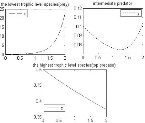
These results obtained by Padé approximations for x(t); y(t) and z(t) are cal-culated and presented follow.
Figure 1. Plots of Padé approximations for a three-species food chain model
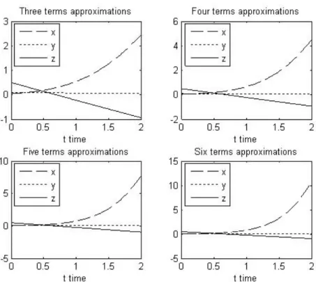
These results obtained by homotopy perturbation method, three, four, …ve and six terms approximations for x(t); y(t) and z(t) are calculated and presented follow.
Figure 2. Plots of three, four, …ve and six terms approximations for a three-species food chain model
5. Conclusions
In this paper, homotopy perturbation method was used for …nding the solutions of nonlinear ordinary di¤erential equation systems such as a three-species food chain model. We demonstrated the accuracy and e¢ ciency of these methods by solving some ordinary di¤erential equation systems. We use Laplace transfor-mation and Padé approximant to obtain an analytic solution and to improve the accuracy of homotopy perturbation method. We apply He’s homotopy pertur-bation method to calculate certain integrals. It is easy and very bene…cial tool for calculating certain di¢ cult integrals or in deriving new integration formula. The computations associated with the examples in this paper were performed using Maple 7 and Matlab 7
References
1. A. Klebano, A .Hastings, Chaos in three species food chains, J Math Biol. 32 (1994) 427–451.
2. P. Katri, S. Ruan, Dynamics of Human T-cell lymphotropic virus I(HTLV-I) infec-tion of CD4+ T-cells, C.R. Biologies 327 (2004) 1009-1016.
3. K. Abboui, Y. Cherruault, New ideas for proving convergence of decomposition methods, Comput. Appl. Math. 29 (7) (1995) 103– 105.
4. G. Adomian, Solving Frontier Problems of Physics: The Decomposition Method, Kluwer, 1994.
5. G. Adomian, A review of the decomposition method in applied mathematics, J. Math. Anal. Appl. 135 (1988) 501–544.
6. J. Biazar, M. Ilie, A. Khoshkenar, A new approach to the solution of the prey and predator problem and comparison of the results with the Adomian method, Applied Mathematics and Computation. 171 (2005) 486–491.
7. J. Biazar, Solution of the epidemic model by Adomian decomposition method, Applied Mathematics and Computation. 173 (2006) 1101–1106.
8. A. M. Wazwaz, A reliable modi…cation of Adomian decomposition method, Appl. Math. Comput. 102 (1999) 77–86.
9. J. H. He, The homotopy perturbation method for nonlinear oscillators with discon-tinuities, Applied Mathematics and Computation 151 (2004) 287–292.
10. J. H. He, Comparison of homotopy perturbation method and homotopy analysis method, Applied Mathematics and Computation 156 (2004) 527–539.
11. J. H. He, Asymptotology by homotopy perturbation method, Applied Mathematics and Computation 156 (3) (2004) 591–596.
12. J. H. He, Homotopy perturbation method for bifurcation of nonlinear problems, International Journal of Non-linear Science Numerical Simulation 6 (2) (2005) 207– 208.
13. J. H. He, Application of homotopy perturbation method to nonlinear wave equa-tions, Chaos, Solitons and Fractals 26 (2005) 695–700.
14. Y. C. Jiao, Y. Yamamoto, C. Dang, Y. Hao, An aftertreatment technique for improving the accuracy of Adomian’s decomposition method, Comput. Math. Appl. 43 (2002) 783–798.
15. S. Momani, Analytical approximate solutions of non-linear oscillators by the mod-i…ed decomposition method, Int. J. Modern Phys. C. 15 (2004) 967–979.
16. J. H. He, Homotopy perturbation method for solving boundary value problems, Physics Letters A 350 (1–2) (2006) 87–88.
17. J. H. He, Semi-inverse method of establishing generalized principles for ‡uid mechanics with emphasis on turbomachinery aerodynamics, International Journal of Turbo Jet-Engines 14 (1997) 23–28.
18. B. A. Finlayson, The Method of Weighted Residuals and Variational Principles, Academic press, New York, 1972.
19. J. H. He, Homotopy perturbation technique, Comput Methods Appl Mech Engrg. 178 (1999) 257–62.
20. J. H. He, A coupling method of a homotopy technique and a perturbation technique for non-linear problems. Int J Non-linear Mech. 35 ( 2000) 37–43.
21. G. A. Baker, Essentials of Pad’e Approximants, Academic Press, London, 1975. 22. Baker G. A., Graves-Morris P. Pade’approdmants. Cambridge: Cambridge Uni-versity Press, 1996.