Volume 2013, Article ID 145967,11pages http://dx.doi.org/10.1155/2013/145967
Research Article
On the Estimations of the Small Periodic Eigenvalues
Seza Dinibütün and O. A. Veliev
Department of Mathematics, Dogus University, Acıbadem, Kadik¨oy, 81010 Istanbul, Turkey
Correspondence should be addressed to Seza Dinib¨ut¨un; [email protected] Received 15 April 2013; Revised 13 June 2013; Accepted 16 June 2013
Academic Editor: Ferhan M. Atici
Copyright © 2013 S. Dinib¨ut¨un and O. A. Veliev. This is an open access article distributed under the Creative Commons Attribution License, which permits unrestricted use, distribution, and reproduction in any medium, provided the original work is properly cited. We estimate the small periodic and semiperiodic eigenvalues of Hill’s operator with sufficiently differentiable potential by two different methods. Then using it we give the high precision approximations for the length of𝑛th gap in the spectrum of Hill-Sehrodinger operator and for the length of𝑛th instability interval of Hill’s equation for small values of 𝑛. Finally we illustrate and compare the results obtained by two different ways for some examples.
1. Introduction
Let𝑃(𝑞) and 𝑆(𝑞) be the operators generated in 𝐿2[0, 𝜋] by the differential expression
−𝑦(𝑥) + 𝑞 (𝑥) 𝑦 (𝑥) (1) with the periodic
𝑦 (𝜋) = 𝑦 (0) , 𝑦(𝜋) = 𝑦(0) (2) and semiperiodic
𝑦 (𝜋) = −𝑦 (0) , 𝑦(𝜋) = −𝑦(0) (3)
boundary conditions, respectively, where𝑞 is a real periodic function with period𝜋. The eigenvalues of 𝑃(𝑞) and 𝑆(𝑞) for𝑞 = 0 are (2𝑛)2 and(2𝑛 + 1)2 for𝑛 ∈ Z, respectively. All eigenvalues of𝑃(0) and 𝑆(0), except 0, are doubled. The eigenvalues of the operators 𝑃(𝑞) and 𝑆(𝑞), called periodic and semiperiodic eigenvalues, are denoted by𝜆2𝑛and𝜆2𝑛+1 for𝑛 ∈ Z, respectively, where
𝜆0(𝑞) < 𝜆−1(𝑞) ≤ 𝜆1(𝑞) < 𝜆−2(𝑞) ≤ 𝜆2(𝑞)
< 𝜆−3(𝑞) ≤ 𝜆3(𝑞) < 𝜆−4(𝑞) ≤ 𝜆4(𝑞) ⋅ ⋅ ⋅ (4) [1, see page 27]. The spectrum𝜎(𝑇(𝑞)) of the operator 𝑇(𝑞) generated in𝐿2[0, 2𝜋] by (1) and the boundary conditions
𝑦 (2𝜋) = 𝑦 (0) , 𝑦(2𝜋) = 𝑦(0) (5)
is the union of the periodic and semiperiodic eigenvalues, that is,
𝜎 (𝑃) = {𝜆2𝑛: 𝑛 ∈ Z} ,
𝜎 (𝑆) = {𝜆2𝑛+1: 𝑛 ∈ Z} , 𝜎 (𝑇) = {𝜆𝑛: 𝑛 ∈ Z} ,
(6)
since (5) holds if and only if either (2) or (3) holds [1, see page 33].
The spectrum of the operator 𝐿(𝑞) generated in 𝐿2(−∞, ∞) by (1) consists of the intervals[𝜆𝑛−1(𝑞), 𝜆−𝑛(𝑞)]
for𝑛 = 1, 2, . . .. Moreover, these intervals are the closure of the stable intervals of equation
−𝑦(𝑥) + 𝑞 (𝑥) 𝑦 (𝑥) = 𝜆𝑦 (𝑥) . (7) The intervals(𝜆−𝑛, 𝜆𝑛) for 𝑛 = 1, 2, . . . are the gaps in the spectrum. These intervals with (−∞, 𝜆0) are the instable intervals of (7) [1, see pages 32 and 82]. The length of𝑛th gap in the spectrum of𝐿(𝑞) (the length of (𝑛 + 1)th instability interval of (7)) is
𝛾𝑛(𝑞) =: 𝜆𝑛(𝑞) − 𝜆−𝑛(𝑞) . (8) Therefore the estimations of the periodic and semiperiodic eigenvalues are also the investigations of the spectrum of𝐿(𝑞) and of the stable intervals of (7).
In this paper we gave the estimations for the small periodic and semiperiodic eigenvalues when the real periodic
potential𝑞 belongs to the Sobolev space 𝑊1𝑘[0, 𝜋] with 𝑘 > 1. These assumptions on the potential𝑞 imply that
𝑞 (𝑥) = ∑ 𝑛∈Z 𝑞𝑛𝑒𝑖2𝑛𝑥, 𝑞−𝑛= 𝑞𝑛, 𝑞𝑛 ≤ 𝑟 (2𝑛)𝑚, (9) where 𝑞𝑛= (𝑞, 𝑒𝑖2𝑛𝑥) = ∫𝜋 0 𝑞 (𝑥) 𝑒 −𝑖2𝑛𝑥𝑑𝑥, 𝑟 = ∫ [0,𝜋]𝑞 (𝑘)(𝑥) 𝑑𝑥. (10)
Without loss of generality, it is assumed that𝑞0= 0. It is wellknown that (see [2])
𝜆𝑛(𝑞) − 𝜆𝑛(0) ≤ sup𝑞(𝑥),
𝜆𝑛(0) = 𝑛2, ∀ 𝑛 ∈ Z. (11) To give a subtle estimate for the eigenvalues𝜆𝑛(𝑞), we write the potential𝑞 in the form
𝑞 (𝑥) = 𝑝 (𝑥) + ∑ |𝑛|>𝑠 𝑞𝑛𝑒𝑖2𝑛𝑥, (12) where 𝑝 (𝑥) = ∑ 𝑛:|𝑛|≤𝑠 𝑞𝑛𝑒𝑖2𝑛𝑥. (13) The inequality in (9) implies that
sup
𝑥∈[0,𝜋]𝑞(𝑥) − 𝑝(𝑥) ≤ ∑|𝑛|>𝑠𝑞𝑛 ≤
𝑟
(𝑘 − 1) (2𝑠)𝑘−1. (14) Hence, by the perturbation theory (see [2]) we have
𝜆𝑛(𝑞) − 𝜆𝑛(𝑝) ≤ (𝑘 − 1) (2𝑠)𝑟 𝑘−1,
𝛾𝑛(𝑞) − 𝛾𝑛(𝑝) ≤ (𝑘 − 1) (2𝑠)2𝑟 𝑘−1.
(15)
Therefore to estimate𝜆𝑛(𝑞) and 𝛾𝑛(𝑞) we can investigate the eigenvalues𝜆𝑛(𝑝) of the operator 𝑇(𝑝) and then use (8) and (15).
In the literature, there are a lot of studies about numerical estimation of the periodic and semiperiodic eigenvalues by using the finite difference method, finite element method, Pr¨ufer transformations, and shooting method. Let us recall some of them. Andrew considered the computations of the eigenvalues by using finite element method [3] and finite difference method [4]. Then these results have been extended by Condon [5] and by Vanden Berghe et al. [6]. Ji and Wong used Pr¨ufer transformation and shooting method in their studies [7–9]. Malathi et al. [10] used shooting technique and direct integration method for computing eigenvalues of periodic Sturm-Liouville problems.
We consider the small periodic and semiperiodic eigen-values by other methods. First, in Section 2, we obtain an
approximation of the eigenvalues𝜆±𝑛(𝑝) for 𝑛 > 𝑚𝑠, where 𝑚 is the positive integer for determination of the error in estimations, by using the method of the paper [11], where the asymptotic formulas for the eigenvalues and eigenfunctions of the 𝑡-periodic boundary value problems were obtained. Then, inSection 3, using it and considering the matrix form of 𝑇(𝑝) we give an approximation with very small errors for all small periodic and semiperiodic eigenvalues. Finally, we apply these investigations to get approximations order 10−18, 10−15, and 10−12 for the first 201 eigenvalues of the
operator 𝑇 with potentials 𝑝1(𝑥) = 2 cos 2𝑥, 𝑝2(𝑥) = 2 cos 2𝑥 + 2 cos 4𝑥, and 𝑝3(𝑥) = 2 cos 2𝑥 + 2 cos 4𝑥 + 2 cos 6𝑥, respectively, and give a comparison between the approxi-mated eigenvalues obtained by the different ways.
2. On Applications of the Asymptotic Methods
In this and next sections, for simplicity of the notation,𝜆𝑛(𝑝) is denoted by𝜆𝑛. By (11)–(13) 𝜆𝑛− 𝑛2 ≤ sup𝑝(𝑥) ≤ 𝑠 ∑ 𝑛=−𝑠𝑞𝑛. (16)To get the subtle estimations for 𝜆𝑛, that is, to observe the influence of the trigonometric polynomial𝑝(𝑥) to the eigenvalue𝑛2of𝑇(0), we use the formula
(𝜆𝑁− 𝑛2) (Ψ𝑁, 𝑒𝑖𝑛𝑥) = (𝑝Ψ𝑁, 𝑒𝑖𝑛𝑥) (17) obtained from the equation
−Ψ𝑁(𝑥) + 𝑝 (𝑥) Ψ𝑁(𝑥) = 𝜆𝑁Ψ𝑁(𝑥) (18) by multiplying 𝑒𝑖𝑛𝑥, where Ψ𝑁 is the eigenfunction corre-sponding to the eigenvalue𝜆𝑛; ‖Ψ𝑛‖ = 1/√𝜋, (⋅, ⋅) and ‖ ⋅ ‖ denote inner product and norm in𝐿2[0, 𝜋].
Introduce the notation 𝑀 = sup 𝑥 𝑝(𝑥), 𝑐 = 𝑠 ∑ 𝑛=−𝑠𝑞𝑛, 𝑄 = sup 𝑛 𝑞𝑛, 𝑋𝑁,𝑛= (Ψ𝑁, 𝑒 𝑖𝑛𝑥) . (19)
Using this notation and (13) in (17) we get (𝜆𝑁− 𝑛2) 𝑋 𝑁,𝑛= 𝑠 ∑ 𝑘=−𝑠 𝑞𝑘𝑋𝑁,𝑛−2𝑘. (20)
In (20) replacing𝑁 by 𝑛 and then iterating it 𝑚 times, as in the paper [11], were done; we obtain
where 𝐴𝑚(𝜆𝑛, 𝑛) =∑𝑚 𝑘=1 𝑎𝑘(𝜆𝑛, 𝑛) , (22) 𝑎𝑘(𝜆𝑛, 𝑛) = ∑𝑠 𝑛1,𝑛2,...,𝑛𝑘=−𝑠 𝑞𝑛1𝑞𝑛2⋅ ⋅ ⋅ 𝑞𝑛𝑘𝑞−𝑛1−𝑛2−⋅⋅⋅−𝑛𝑘 ∏𝑖=1,2,...,𝑘[𝜆𝑛− (𝑛 − 2𝑛1− 2𝑛2⋅ ⋅ ⋅ − 2𝑛𝑖)2], 𝑅𝑚+1(𝜆𝑛, 𝑛) = ∑𝑠 𝑛1,𝑛2,...,𝑛𝑚+1=−𝑠 × 𝑞𝑛1𝑞𝑛2⋅ ⋅ ⋅ 𝑞𝑛𝑚𝑞𝑛𝑚+1𝑋𝑛,𝑛−2𝑛1−2𝑛2−⋅⋅⋅−2𝑛𝑚+1 ∏𝑖=1,2,...𝑚[𝜆𝑛− (𝑛 − 2𝑛1− 2𝑛2⋅ ⋅ ⋅ − 2𝑛𝑖)2] , (23) 𝑛𝑗 ̸= 0, ∀ 𝑗,∑𝑘 𝑗=1 𝑛𝑗 ̸= 0, ∀ 𝑘 = 1, 2, . . . , 𝑚 (24) under assumption that
𝜆𝑛− (𝑛 − 2𝑛1⋅ ⋅ ⋅ − 2𝑛𝑖)2 ̸= 0 (25) for𝑖 = 1, 2, . . . , 𝑚. Now using (21), estimating𝑋𝑛,𝑛and𝑅𝑚+1, we prove the following,
Theorem 1. Let 𝑚 be a positive integer. If the conditions
|𝑛| > 𝑚𝑠, 4 (|𝑛| − 1) ≥ 3𝑀 (26)
hold, then the eigenvalue𝜆𝑛of the operator𝑇(𝑝) satisfies 𝜆𝑛= 𝑛2 +∑𝑚 𝑘=1 𝑠 ∑ 𝑛1,𝑛2,...,𝑛𝑘=−𝑠 × 𝑞𝑛1𝑞𝑛2⋅ ⋅ ⋅ 𝑞𝑛𝑘𝑞−𝑛1−𝑛2−⋅⋅⋅−𝑛𝑘 ∏𝑖=1,2,...𝑘[𝜆𝑛− (𝑛 − 2𝑛1− 2𝑛2⋅ ⋅ ⋅ − 2𝑛𝑖)2] + 𝛼𝑛,𝑚, (27) where 𝛼𝑛,𝑚 ≤ 2𝑐 𝑚+1 (4 (|𝑛| − 1) − 𝑀)𝑚; (28)
𝑐, 𝑀, and 𝑝(𝑥) are defined in (19) and (13).
Proof. Since𝑞0 = 0 we have 0 < |𝑛𝑖| ≤ 𝑠. This with (16), (19),
and (26) implies that
𝜆𝑛− (𝑛 − 2𝑛1− 2𝑛2− ⋅ ⋅ ⋅ − 2𝑛𝑖)2
≥ 𝑛2− (|𝑛| − 2)2 − 𝑀 = 4 (|𝑛| − 1) − 𝑀 ≥ 2𝑀 > 0
(29)
for𝑖 = 1, 2, . . . , 𝑚; that is, assumption (25) holds. Therefore we can use (21).
Now we estimate𝑋𝑛,𝑛and𝑅𝑚+1. First let us estimate𝑅𝑚+1. Since‖Ψ𝑛‖ = 1/√𝜋 by Schwarz inequality we have
(Ψ𝑛(𝑥) , 𝑒𝑖(𝑛−2𝑛1−2𝑛2−⋅⋅⋅−2𝑛𝑚+1)𝑥) ≤ 1. (30)
This with (23) and (29) implies that 𝑅𝑚+1 ≤ (4 (|𝑛| − 1) − 𝑀)1 𝑚 × ∑𝑠 𝑛1,𝑛2,...,𝑛𝑚+1=−𝑠 𝑞𝑛1𝑞𝑛2⋅ ⋅ ⋅ 𝑞𝑛𝑚𝑞𝑛𝑚+1 . (31)
Hence by definition of𝑐 (see (19)) we have 𝑅𝑚+1 ≤ 𝑐
𝑚+1
(4 (|𝑛| − 1) − 𝑀)𝑚. (32)
Now we estimate𝑋𝑛,𝑛. Arguing as in the proof of (29) we get
𝜆𝑛− (𝑛 − 2𝑘)2 ≥ 2𝑀, ∀𝑘 ̸= 0, 𝑛. (33)
Therefore using (17) we get ∑ 𝑘∈Z,𝑘 ̸= 0,𝑛𝑋𝑛,𝑛−2𝑘 2= ∑ 𝑘∈Z,𝑘 ̸= 0,𝑛 (Ψ𝑛, 𝑝𝑒𝑖((𝑛−2𝑘))𝑥)2 𝜆𝑛− (𝑛 − 2𝑘)22 ≤ 𝑀2 (2𝑀)2 = 1 4. (34)
This with Parseval’s equality ∑ 𝑘∈Z𝑋𝑛,𝑛−2𝑘 2= ∑ 𝑘∈Z,(Ψ𝑛 , 𝑒𝑖((𝑛−2𝑘))𝑥)2= 1 (35) implies that 𝑋𝑛,𝑛2+ 𝑋𝑛,−𝑛2≥34. (36)
Hence at least one of the inequalities
𝑋𝑛,𝑛 ≥ 12, 𝑋𝑛,−𝑛 ≥ 12 (37)
holds. If the first inequality holds, then dividing both sides of (21) by𝑋𝑛,𝑛and using (23), (32) we obtain the proof of (27) and (28). If the second inequality holds, then instead of (21) using
(𝜆𝑛− (−𝑛)2) 𝑋𝑛,−𝑛= 𝐴𝑚(𝜆𝑛, −𝑛) 𝑋𝑛,−𝑛+ 𝑅𝑚+1(𝜆𝑛, −𝑛) , (38) taking into account that𝐴𝑚(𝜆𝑛, −𝑛) = 𝐴𝑚(𝜆𝑛, 𝑛) and arguing as in the first case we get the proof in the second case. Theorem is proved.
Now using (27) let us show that𝜆±𝑛is close to the root of the equation 𝑥 = 𝑛2+ 𝑓 (𝑥) , (39) where 𝑓 (𝑥) = ∑𝑠 𝑛1=−𝑠 𝑞𝑛1𝑞−𝑛1 𝑥 − (𝑛 − 2𝑛1)2 + ∑𝑠 𝑛1,𝑛2=−𝑠 𝑞𝑛1𝑞𝑛2𝑞−𝑛1−𝑛2 (𝑥 − (𝑛 − 2𝑛1)2) (𝑥 − (𝑛 − 2𝑛1− 2𝑛2)2) + . . . + ∑𝑠 𝑛1,𝑛2,...𝑛𝑚=−𝑠 × ((𝑞𝑛1𝑞𝑛2⋅ ⋅ ⋅ 𝑞𝑛𝑚𝑞−𝑛1−𝑛2−⋅⋅⋅−𝑛𝑚) × ([𝑥 − (𝑛 − 2𝑛1)2] [𝑥 − (𝑛 − 2𝑛1− 2𝑛2)2] ⋅ ⋅ ⋅ [𝑥 − (𝑛 − 2𝑛1− 2𝑛2− ⋅ ⋅ ⋅ − 2𝑛𝑚)2] )−1) . (40)
Theorem 2. Let 𝑛 be a positive integer satisfying
𝑛 > 𝑚𝑠, 4 (𝑛 − 1) > 𝑀 + 2𝑐. (41)
Then for all𝑥 and 𝑦 from [𝑛2− 𝑀, 𝑛2+ 𝑀] the inequality
𝑓(𝑥) − 𝑓(𝑦) < 𝐾𝑛𝑥 − 𝑦, (42)
where
𝐾𝑛= (4 (𝑛 − 1) − 𝑀) (4 (𝑛 − 1) − 𝑀 − 𝑐)𝑄𝑐 < 12, (43)
holds, and (39) has a unique solution𝑟𝑛on[𝑛2− 𝑀, 𝑛2+ 𝑀]. Moreover
𝜆±𝑛− 𝑟𝑛 < 2𝑐 𝑚+1
(1 − 𝐾𝑛) (4 (𝑛 − 1) − 𝑀)𝑚 (44)
and the length𝛾𝑛of𝑛th gap in the spectrum of 𝐿(𝑝) (the length
𝛾𝑛of(𝑛 + 1)th instability interval of (7)) satisfies
𝛾𝑛 = 𝜆𝑛− 𝜆−𝑛< 4𝑐𝑚+1
(1 − 𝐾𝑛) (4 (𝑛 − 1) − 𝑀)𝑚. (45)
Proof. Let𝑓1(𝑥),𝑓2(𝑥), . . .,𝑓𝑚(𝑥) be the first, second, and 𝑚th
summations in the right-hand side of (40). Then 𝑓1(𝑥) = −∑𝑠
𝑘=−𝑠
𝑞2𝑘
(𝑥 − (𝑛 − 2𝑘)2)2. (46) For𝑥 ∈ [𝑛2− 𝑀, 𝑛2+ 𝑀], using (29) and (41), we get
𝑥 − (𝑛 − 2𝑘)2 ≥ 4 (𝑛 − 1) − 𝑀 > 2𝑐. (47)
On the other hand
𝑠
∑
𝑘=−𝑠𝑞
2
𝑘 ≤ 𝑄𝑐. (48)
This inequality with (47) and the inequality𝑄 ≤ 𝑐 (see (19)) imply that
𝑓1(𝑥) ≤ (4 (𝑛 − 1) − 𝑀)𝑄𝑐 2 <
1
4. (49)
In the same way we obtain 𝑓𝑘(𝑥) ≤ 𝑄𝑐 𝑘 (4 (𝑛 − 1) − 𝑀)𝑘+1 < 1 2𝑘+1 (50)
for𝑘 = 2, 3, . . . . Thus by the geometric series formula we have
𝑓(𝑥) ≤ 𝐾𝑛< 12, ∀ 𝑥 ∈ [𝑛2− 𝑀, 𝑛2+ 𝑀] , (51)
where𝐾𝑛is defined in (43), and by mean-value theorem (42) holds. Therefore by contraction mapping theorem (39) has a unique solution𝑟𝑛on[𝑛2− 𝑀, 𝑛2+ 𝑀].
Now let us prove (44). Let𝐹(𝑥) = 𝑥−𝑛2−𝑓(𝑥). Using the definition of𝑟𝑛and𝐹(𝑥) and then (40) we obtain𝐹(𝑟𝑛) = 0 and
𝐹(𝜆𝑛) − 𝐹 (𝑟𝑛) ≤𝛼𝑛,𝑚. (52)
On the other hand by (51) we have|𝐹(𝑥)| ≥ 1 − 𝐾𝑛for all 𝑥 ∈ [𝑛2−𝑀, 𝑛2+𝑀]. Therefore using the mean-value formula
𝐹(𝜆𝑛) − 𝐹 (𝑟𝑛) =𝐹(𝜁)𝜆𝑛− 𝑟𝑛, (53)
𝜁 ∈ [𝑛2− 𝑀, 𝑛2+ 𝑀], and (52) we obtain
𝜆𝑛− 𝑟𝑛 ≤1 − 𝐾𝛼𝑛,𝑚
𝑛. (54)
This with (28) implies (44) for𝜆𝑛. In the same way we prove (44) for𝜆−𝑛. Therefore (45) follows from (44). The theorem is proved.
Now let us approximate𝑟𝑛by fixed-point iteration 𝑥𝑛,0= 𝑛2, 𝑥𝑛,1= 𝑛2+ 𝑓 (𝑥𝑛,0) , . . . , 𝑥𝑛,𝑖= 𝑛2+ 𝑓 (𝑥𝑛,𝑖−1) .
(55) Note that repeating the proof of (51) one can readily see that 𝑓(𝜆𝑛) ≤ 4 (𝑛 − 1) − 𝑀 − 𝑐𝑄𝑐 , 𝑓 (𝑛2) ≤ 4 (𝑛 − 1) − 𝑐𝑄𝑐
(56) for all𝑛 satisfying (41).
Theorem 3. For the sequence {𝑥𝑛,𝑖} defined by (55) the
estimations
𝑥𝑛,𝑖− 𝑟𝑛 ≤ 𝐾𝑛𝑖𝐵 (57)
for𝑖 = 1, 2, 3, . . . hold, where 𝑛 satisfies (41),𝐾𝑛is defined in
Theorem 2, and 𝐵 = 𝑓 (𝑛 2 ) 1 − 𝐾𝑛 ≤ 𝑄𝑐 (1 − 𝐾𝑛) (4 (𝑛 − 1) − c). (58)
Proof. It is clear and well known that if𝑓 satisfies (42) then
𝑥𝑛,𝑖− 𝑟𝑛 ≤ 𝐾𝑖𝑛𝑥𝑛,0− 𝑟𝑛. (59)
Therefore to prove (57) it is enough to show that
𝑥𝑛,0− 𝑟𝑛 ≤ 𝐵, (60)
where𝐵 is defined in (58). By definition of𝑟𝑛and𝑥𝑛,0we have 𝑟𝑛− 𝑥𝑛,0= 𝑓 (𝑟𝑛) = 𝑓 (𝑟𝑛) − 𝑓 (𝑥𝑛,0) + 𝑓 (𝑛2) , (61) and by the mean-value theorem there exists𝑥 ∈ [𝑛2−𝑀, 𝑛2+ 𝑀] such that
𝑓 (𝑟𝑛) − 𝑓 (𝑥𝑛,0) = 𝑓(𝑥) (𝑟𝑛− 𝑥𝑛,0) . (62) These two equalities imply that
(𝑟𝑛− 𝑥𝑛,0) (1 − 𝑓(𝑥)) = 𝑓 (𝑛2) . (63) This formula with (56) and (51) implies (60).
Thus by (44) and (57) we have the approximation𝑥𝑛,𝑖for 𝜆±𝑛with the error
𝐸𝑛,𝑖=: 𝜆±𝑛− 𝑥𝑛,𝑖 < 2𝑐𝑚+1
(1 − 𝐾𝑛) (4 (𝑛 − 1) − 𝑀)𝑚 + 𝐾𝑖𝑛𝐵. (64)
3. Estimation of the Small Eigenvalues
In this section we estimate the eigenvalues𝜆𝑁of the operator 𝑇(𝑝), for |𝑁| ≤ 𝑙, by investigating the system of 2𝑆 + 1 equations (𝜆𝑁− 𝑛2) 𝑋𝑁,𝑛− ∑ 𝑘:|𝑘|≤𝑠,|𝑛−2𝑘|≤𝑆 𝑞𝑘𝑋𝑁,𝑛−2𝑘 = ∑ 𝑘:|𝑘|≤𝑠,|𝑛−2𝑘|>𝑆 𝑞𝑘𝑋𝑁,𝑛−2𝑘 (65)
for𝑛 = −𝑆, −𝑆 + 1, −𝑆 + 2, . . . , 𝑆, where 𝑆 = 𝑙 + 2𝑟𝑠 and 𝑟 is the positive integer for determination of the error in estimation, 4 (𝑙 − 1) − 𝑀 − 𝑐 > max {𝑐, 2𝑐2} ; (66) the numbers𝑀 and 𝑐 are defined in (19). The first, second, and𝑗th equations of (65) are obtained from (20) by taking 𝑛 = −𝑆, 𝑛 = −𝑆 + 1, and 𝑛 = −𝑆 − 1 + 𝑗, respectively, and by writing the terms with multiplicand𝑋𝑁,𝑛−2𝑘for|𝑛 − 2𝑘| ≤ 𝑆 on the left-hand side and the terms with multiplicand𝑋𝑁,𝑛−2𝑘 for|𝑛 − 2𝑘| > 𝑆 on the right-hand side.
To write (65) in the matrix form let us introduce the notations. Let𝐴 be (2𝑆 + 1) by (2𝑆 + 1) matrix (𝑎𝑖,𝑗) defined by
𝑎𝑖,𝑖 = (−𝑆 − 1 + 𝑖)2, 𝑎𝑖,𝑖∓2𝑘= 𝑞±𝑘 (67) for 𝑖 = 1, 2, . . . , 2𝑆 + 1 and 𝑘 = 1, 2, . . . 𝑠 if |𝑖 ∓ 2𝑘| ≤ 𝑆 and all other entries of 𝐴 are zero. Since 𝑞−𝑛 = 𝑞𝑛
(see (9)), 𝐴 is a Hermitian (self-adjoint) matrix and its eigenvalues are real numbers. Denote the eigenvalues of𝐴 by 𝜇0, 𝜇−1, 𝜇1, 𝜇−2, 𝜇2, . . . , 𝜇−𝑆, 𝜇𝑆, where
𝜇0≤ 𝜇−1 ≤ 𝜇1≤ 𝜇−2 ≤ 𝜇2≤ ⋅ ⋅ ⋅ ≤ 𝜇−𝑆≤ 𝜇𝑆. (68) It is clear that
𝜇±𝑛− 𝑛2 ≤ 𝑐, (69)
since the diagonal elements of𝐴 are 𝑛2for𝑛 = −𝑆, −𝑆+1, −𝑆+ 2, . . . , 𝑆 and the sum of the absolute values of the nondiagonal elements of each row is not greater than𝑐 (see (19)). Let𝑋𝑁=
(𝑋𝑁,−𝑆, 𝑋𝑁,−𝑆+1, . . . , 𝑋𝑁,𝑆) and 𝑅(𝜆N) = (𝑅−𝑆, 𝑅−𝑆+1, . . . , 𝑅𝑆)
be vectors ofC2𝑆+1, where𝑅𝑛= 0 for |𝑛| ≤ 𝑆 − 2𝑠 and 𝑅𝑛(𝜆𝑁) = ∑
𝑘:|𝑘|≤𝑠, |𝑛−2𝑘|>𝑆
𝑞𝑘𝑋𝑁,𝑛−2𝑘 (70)
for𝑆 − 2𝑠 < |𝑛| ≤ 𝑆. In this notation the system of (65) can be written in the matrix form
(𝜆𝑁𝐼 − 𝐴) 𝑋𝑇𝑁= 𝑅𝑇(𝜆𝑁) . (71) First we prove that𝑋𝑁,𝑛for𝑛 = ±(𝑆+1), ±(𝑆+2), . . . , ±(𝑆+ 2𝑠), that is, the right-hand side 𝑅𝑇(𝜆
𝑁) of (71), is small (see
Lemma 4). Then using it we prove that the𝑛th eigenvalue 𝜆𝑛 of the operator𝑇(𝑝) is close to the 𝑛th eigenvalue 𝜇𝑛of the matrix𝐴 (seeTheorem 6).
Lemma 4. If |𝑁| ≤ 𝑙 and 𝑙 + 2𝑟𝑠 < |𝑛| ≤ 𝑙 + 2(𝑟 + 1)𝑠, then
𝑋𝑁,𝑛 ≤ 𝑐 𝑟+1 (2𝑙)𝑟+1 =: 𝜀, (72) ∑ 𝑛:|𝑛|>𝑆𝑋𝑁,𝑛 2≤ 4𝑠𝜀2(2𝑙)2 ((2𝑙)2− 𝑐2) = 4𝑠𝑐2𝑟+2 (2𝑙)2𝑟((2𝑙)2− 𝑐2) =: 𝛿. (73)
Proof. First we prove (72) for positive 𝑛. The proof for negative𝑛 is similar. One can readily see from the estimations (27), (28) for𝑚 = 2, (56), and (66) that if𝑘 ≥ 𝑙, then
𝜆𝑘− 𝑘2 ≤ 𝑓(𝜆𝑘) +𝛼𝑘,2 ≤ 𝑄𝑐 4 (𝑘 − 1) − 𝑀 − 𝑐+ 2𝑐3 (4 (𝑘 − 1) − 𝑀)2 < 1. (74)
Using (74) and taking into account the condition on𝑁 and 𝑛 we obtain 𝜆𝑁− (𝑛 − 2𝑛1− ⋅ ⋅ ⋅ − 2𝑛𝑖)2 ≥ 𝜆𝑁− (𝑙 + 1)2 ≥ 𝜆𝑙− (𝑙 + 1)2 >𝑙2− (𝑙 + 1)2 − 1 ≥ 2𝑙 (75)
for|𝑛𝑖| ≤ 𝑠, 𝑖 = 0, 1, . . . , 𝑟. On the other hand iterating (20)𝑟 times we get 𝑋𝑁,𝑛= ∑𝑠 𝑛1,𝑛2,...,𝑛𝑟=−𝑠 × ((𝑞𝑛1𝑞𝑛2⋅ ⋅ ⋅ 𝑞𝑛𝑟+1(Ψ𝑁, 𝑒𝑖(𝑛−2𝑛1−⋅⋅⋅−2𝑛2𝑟+1)𝑥)) × ([𝜆𝑁− 𝑛2] [𝜆𝑁− (𝑛 − 2𝑛1)2] ⋅ ⋅ ⋅ [𝜆𝑁− (𝑛 − 2𝑛1− ⋅ ⋅ ⋅ − 2𝑛𝑟)2])−1) . (76) Therefore arguing as in the proof of (32) we get
𝑋𝑁,𝑛 ≤ 𝑐 𝑟+1
(2𝑙)𝑟+1 (77)
for𝑙 + 2𝑟𝑠 < |𝑛| ≤ 𝑙 + 2(𝑟 + 1)𝑠; that is, (72) is proved. Now we prove (73). By definition of𝑆 the left-hand side of (73) can be written in the form
∑ 𝑛:|𝑛|>𝑆𝑋𝑁,𝑛 2=∑∞ 𝑘=𝑟 𝐻𝑁,𝑘, (78) where 𝐻𝑁,𝑘= ∑ 𝑙+2𝑘𝑠<|𝑛|≤𝑙+2(𝑘+1)𝑠,𝑋𝑁,𝑛 2. (79) In (72) replacing𝑟 by 𝑘 one can readily see that
𝐻𝑁,𝑘≤ 4𝑠𝑐2𝑘+2
(2𝑙)2𝑘+2. (80)
Using this in (78) we obtain ∑ 𝑛:|𝑛|>𝑆𝑋𝑁,𝑛 2≤∑∞ 𝑘=𝑟 4𝑠𝑐2𝑘+2 (2𝑙)2𝑘+2 (81)
which implies (73), since the series in the right-hand side of (81) is a geometric series with first term4𝑠𝜀2 and factor 𝑐2/(2𝑙)2.
Note that (72) and (73) imply the following inequalities. By (70) and (72)
𝑅𝑛(𝜆𝑁) < 𝑐𝜀, ∀𝑛 : 𝑆 − 2𝑠 < |𝑛| ≤ 𝑆, ∀ |𝑁| ≤ 𝑙, (82)
and by the definition of𝑅(𝜆𝑁) we have
𝑅(𝜆𝑁) ≤ 2𝑐𝜀√𝑠, ∀ |𝑁| ≤ 𝑙. (83)
Besides using (73) and Parseval’s equality (35) we obtain 1 − 𝛿 ≤ ∑𝑆
𝑛=−𝑆𝑋𝑁,𝑛
2≤ 1,
√1 − 𝛿 ≤ 𝑋𝑁 ≤ 1, ∀|𝑁| ≤ 𝑙.
(84)
Let{𝑉𝑛𝑇 : 𝑛 = 0, ±1, ±2, . . . , ±𝑆} be orthonormal system of eigenvectors of the matrix𝐴:
𝐴𝑉𝑛𝑇= 𝜇𝑛𝑉𝑛𝑇, (85) where⟨𝑉𝑛, 𝑉𝑘⟩ = 𝛿𝑛,𝑘, 𝑉𝑛 = (𝑉𝑛,−𝑆, 𝑉𝑛,−𝑆+1, . . . , 𝑉𝑛,𝑆) ∈ C2𝑆+1, and⟨⋅, ⋅⟩ denotes the inner product in C2𝑆+1as well as in𝑙2. Denote by𝐷 the (2𝑆 + 1) × (2𝑆 + 1) diagonal matrix with diagonal elements
𝑑𝑖= 𝑎𝑖,𝑖= (−𝑆 − 1 + 𝑖)2 (86) for 𝑖 = 1, 2, . . . , 2𝑆 + 1. The eigenfunctions of 𝐷 corre-sponding to the eigenvalues𝑛2 are𝑒−𝑛 and 𝑒𝑛, where𝑒𝑛 =
(𝑒𝑛,−𝑆, 𝑒𝑛,−𝑆+1, . . . , 𝑒𝑛,𝑆)𝑇, 𝑒𝑛,𝑛 = 1, and 𝑒𝑛,𝑘 = 0 for all 𝑘 ̸= 𝑛.
Multiplying both sides of (85) for𝑛 = 𝑁 by 𝑒𝑛we get (𝜇𝑁− 𝑛2) 𝑉𝑁,𝑛= ∑𝑠
𝑘=−𝑠
𝑞𝑘𝑉𝑁,𝑛−2𝑘, (87)
where𝑉𝑁,𝑛−2𝑘= 0 if |𝑛 − 2𝑘| > 𝑆. Instead of (20) using (87) and repeating the proof of (72) we obtain that if|𝑁| ≤ 𝑙 and |𝑛| > 𝑆 − 2𝑠, then
𝑉𝑁,𝑛 ≤ 𝑐 𝑟
(2𝑙)𝑟. (88)
To prove the main result of the paper we use the following.
Lemma 5. Let 𝑐𝑛,𝑗 = ⟨𝑋𝑇 𝑛, 𝑉𝑗𝑇⟩ and 𝑛 = 0, ±1, ±2, . . . , ±𝑙. Then 𝑐𝑛,𝑗(𝜇𝑗− 𝜆𝑛) ≤ 8𝑠𝑙𝜀2 (89) for𝑗 = 0, ±1, ±2, . . . , ±𝑙 and 𝑐𝑛,𝑗(𝜇𝑗− 𝜆𝑛) ≤ 2𝑐𝜀√𝑠 (90) for𝑗 = ±(𝑙 + 1), ±(𝑙 + 2), . . . , ±𝑆.
Proof. Since{𝑉𝑗 : 𝑗 = 0, ±1, ±2, . . . , ±𝑆} is an orthonormal
basis inC2𝑆+1we have 𝑋𝑇𝑛 = ∑𝑆 𝑗=−𝑆 𝑐𝑛,𝑗𝑉𝑗𝑇, 𝑋𝑘2= ∑𝑆 𝑗=−𝑆𝑐𝑘,𝑗 2 . (91)
Using this in (71) we get
𝑅𝑇(𝜆𝑛) = (𝜆𝑛𝐼 − 𝐴) 𝑋𝑇𝑛 = ∑𝑆 𝑗=−𝑆 (𝜆𝑛𝑐𝑛,𝑗𝑉𝑗𝑇− 𝐴 (𝑐𝑛,𝑗𝑉𝑗𝑇)) = ∑𝑆 𝑗=−𝑆 𝑐𝑛,𝑗(𝜆𝑛− 𝜇𝑗) 𝑉𝑇 𝑗 . (92)
Multiplying both sides by𝑉𝑗𝑇we obtain
On the other hand using the definition𝑅𝑇(𝜆𝑛), (82), and (88) we get ⟨𝑅𝑇(𝜆𝑛) , 𝑉𝑗𝑇⟩ ≤ 4𝑠𝑐𝜀 𝑐 𝑟 (2𝑙)𝑟 = 8𝑠𝑙𝜀2 (94) for all𝑛, 𝑗 = 0, ±1, ±2, . . . , ±𝑙. This with (93) implies (89).
By Schwarz inequality and (83) we have
⟨𝑅𝑇(𝜆𝑛) , 𝑉𝑗𝑇⟩ ≤ 2𝑐𝜀√𝑠 (95)
for all 𝑛 = 0, ±1, ±2, . . . , ±𝑙 and 𝑗 = 0, ±1, ±2, . . . , ±𝑆. Therefore (90) follows from (93).
Introduce the notation
𝑌𝑛= (⋅ ⋅ ⋅ 𝑋𝑛,−𝑆−1, 𝑋𝑛,−𝑆, 𝑋𝑛,−𝑆+1, . . . , 𝑋𝑛,𝑆, 𝑋𝑛,𝑆+1, . . .) , 𝑈𝑗= (⋅ ⋅ ⋅ 0, 0, 𝑉𝑗,−𝑆, 𝑉𝑗,−𝑆+1, . . . , 𝑉𝑗,𝑆, 0, 0, . . .) . (96) Here𝑌𝑛and𝑈𝑗are elements of𝑙2, and
⟨𝑌𝑛, 𝑈𝑗⟩ = ∑∞ 𝑖=−∞ 𝑋𝑛,𝑖𝑉𝑗,𝑖= ∑𝑆 𝑖=−𝑆 𝑋𝑛,𝑖𝑉𝑗,𝑖= ⟨𝑋𝑇𝑛, 𝑉𝑗𝑇⟩ = 𝑐𝑛,𝑗. (97) Using equality (35) and the definition of𝑌𝑛 and𝑈𝑗 one can easily verify that{𝑌𝑛 : 𝑛 = 0, ±1, ±2, . . . , ±𝑆} and {𝑈𝑛 : 𝑛 = 0, ±1, ±2, . . . , ±𝑆} are the orthonormal systems in 𝑙2.
Now we are ready to prove the following main result.
Theorem 6. If 𝑙 > max{𝑐2, 2𝑐, 3𝑠} then the inequality
𝜆𝑛− 𝜇𝑛 ≤ 8𝑆𝑠𝑐 2𝑟+2
(2𝑙)2𝑟+1 (98)
holds for all𝑛 = 0, ±1, ±2, . . . , ±𝑙, where 𝑆, 𝑟, 𝑙 and 𝑐, 𝑠 are defined in (65) and (19).
Proof. Suppose to the contrary and without loss of generality
that (98) does not hold for some0 ≤ 𝑛 ≤ 𝑙. Then either 𝜆𝑛 < 𝜇𝑛− (8𝑆𝑠𝑐2𝑟+2/(2𝑙)2𝑟+1) or 𝜆𝑛 > 𝜇𝑛+ (8𝑆𝑠𝑐2𝑟+2/(2𝑙)2𝑟+1). Let
us consider the case𝜆𝑛< 𝜇𝑛− (8𝑆𝑠𝑐2𝑟+2/(2𝑙)2𝑟+1). Then 𝜆𝑘 < 𝜇𝑗−8𝑆𝑠𝑐2𝑟+2
(2𝑙)2𝑟+1, (99)
and hence by (89)|𝑐𝑘,𝑗| < 1/2𝑆 for all 𝑘 = 0, ±1, ±2, . . . , ±𝑛, 𝑗 = 𝑛, ±(𝑛 + 1), ±(𝑛 + 2) . . . , ±𝑙. It implies that
𝑐𝑘,𝑛2+ ∑
𝑗:𝑛<|𝑗|≤𝑙𝑐𝑘,𝑗
2
≤ 2𝑙 + 1 − 2𝑛4𝑆2 (100) for𝑘 = 0, ±1, ±2, . . . , ±𝑛. On the other hand from Parseval’s equality (91) we have 𝑛 ∑ 𝑘=−𝑛𝑋𝑘 2= ∑𝑛 𝑘=−𝑛 𝑆 ∑ 𝑗=−𝑆𝑐𝑘,𝑗 2 . (101)
Now we are going to get a contradiction by proving that the left-hand side of (101) is greater than the right-hand side of (101). Using (84), the definition of𝛿, and the conditions on 𝑙 one can easily verify that
𝑛
∑
𝑘=−𝑛𝑋𝑘
2≥ 2𝑛 + 1 − (2𝑛 + 1) 𝛿 > 2𝑛 +3
4. (102)
To estimate the right-hand side of (101) we write it as𝑆1+𝑆2+ 𝑆3, where 𝑆1= ∑𝑛 𝑘=−𝑛(𝑐𝑘,𝑛 2+ ∑ 𝑗:𝑛<|𝑗|≤𝑙𝑐𝑘,𝑗 2 ) , 𝑆2= ∑𝑛 𝑘=−𝑛 𝑛−1 ∑ 𝑗=−𝑛𝑐𝑘,𝑗 2 , 𝑆3= ∑𝑛 𝑘=−𝑛 ( ∑ 𝑗:|𝑗|>𝑙𝑐𝑘,𝑗 2 ) . (103)
Using (100) and taking into account that(2𝑙+1−2𝑛)+(2𝑛+1) ≤ 2𝑆 and hence (2𝑙 + 1 − 2𝑛)(2𝑛 + 1) ≤ 𝑆2we obtain
𝑆1≤ (2𝑙 + 1 − 2𝑛) (2𝑛 + 1)4𝑆2 <14. (104) Now let us estimate 𝑆3. Using (99), (69), and then the inequality𝑙 > 2𝑐 we obtain
𝜆𝑘− 𝜇𝑗 >𝜇𝑙− 𝜇𝑗 >𝑗 (105)
for𝑘 = 0, ±1, ±2, . . . , ±𝑛 and |𝑗| > 𝑙. Therefore this, (90), and the definition𝜀 imply that
𝑆3= 𝑛 ∑ 𝑘=−𝑛 ( ∑ 𝑗:|𝑗|>𝑙𝑐𝑘,𝑗 2 ) ≤ (2𝑛 + 1) ∑ 𝑗:|𝑗|>𝑙 (2𝑐𝜀√𝑠 𝑗 ) 2 < (2𝑛 + 1)4𝑠𝑐𝑙2𝜀2 < 1 4. (106)
Now let us estimate𝑆2. Using (97) and the Bessel inequal-ity for the elements𝑈𝑖for𝑖 = −𝑛, −𝑛+1, . . . , 𝑛−1 with respect to the orthonormal systems{𝑌𝑛 : 𝑛 = 0, ±1, ±2, . . . , ±𝑛} of 𝑙2 we obtain 𝑛 ∑ 𝑘=−𝑛𝑐𝑘,𝑖 2 ≤ 𝑈𝑖2= 1, 𝑆2= 𝑛−1 ∑ 𝑖=−𝑛 𝑛 ∑ 𝑘=−𝑛𝑐𝑘,𝑖 2≤ 2𝑛. (107)
The inequalities (104)–(107) show that the right side of (101) is less than2𝑛 + (1/2), which contradicts (102). In the same way we investigate the case𝜆𝑛> 𝜇𝑛+ (8𝑆𝑠𝑐2𝑟+2/(2𝑙)2𝑟+1). The theorem is proved.
4. Examples and Conclusion
In this section we illustrate the results of Sections2and3for the following examples. Let the potential𝑝𝑠(𝑥) for 𝑠 = 1, 2, 3 of the operator𝑇(𝑝𝑠) have the form
𝑝𝑠(𝑥) =∑𝑠
𝑛=1
(𝑒𝑖2𝑛𝑥+ 𝑒−𝑖2𝑛𝑥) =∑𝑠
𝑛=1
Table 1: Estimations for𝑇(𝑝1). 𝑥𝑛,3 𝐸𝑛,3 𝛾𝑛 𝑛 = 7 49.0119073043627 0.00401827341683563 0.00803652968036530 𝑛 = 8 64.0090356900908 0.00232226049016466 0.00464451589853519 𝑛 = 9 81.0070967373201 0.00146120590904089 0.00292241001412498 𝑛 = 10 100.005724155838 0.00097836132370372 0.00195672191528545 𝑛 = 20 400.001412301984 8.57660779334148× 10⁻⁵ 0.00017153215300668 𝑛 = 30 900.000626190365 2.27805363772165× 10⁻⁵ 4.55610726195539× 10⁻⁵ 𝑛 = 40 1600.00035193858 9.11289409047171× 10⁻⁶ 1.82257881647412× 10⁻⁵ 𝑛 = 50 2500.00022515394 4.5213654576927× 10⁻⁶ 9.04273091219341× 10⁻⁶ 𝑛 = 60 3600.00015632421 2.56272510680566× 10⁻⁶ 5.12545021275656× 10⁻⁶ 𝑛 = 70 4900.00011483597 1.59021161389524× 10⁻⁶ 3.18042322750835× 10⁻⁶ 𝑛 = 80 6400.0000879141 1.05364682405463× 10⁻⁶ 2.10729364800086× 10⁻⁶ 𝑛 = 90 8100.0000694591 7.33717636691826× 10⁻⁷ 1.46743527333693× 10⁻⁶ 𝑛 = 100 10000.0000562596 5.31248113844258× 10⁻⁷ 1.06249622766647× 10⁻⁶
Table 2: Estimations for𝑇(𝑝2).
𝑥𝑛,3 𝐸𝑛,3 𝛾𝑛 𝑛 = 13 169.006553875546 0.00801822430426367 0.01603644646924830 𝑛 = 14 196.005629484083 0.00602192413268590 0.01204384713096120 𝑛 = 15 225.004888933687 0.00463706113393842 0.00927412163367219 𝑛 = 16 256.004286247051 0.00364633797625785 0.00729267558174552 𝑛 = 17 289.003789043447 0.00291892692052321 0.00583785361582058 𝑛 = 18 324.003373962035 0.00237284215158748 0.00474568416174256 𝑛 = 19 361.003023794203 0.00195492184884340 0.00390984360625575 𝑛 = 20 400.002725629827 0.00162966444959707 0.00325932883855288 𝑛 = 30 900.001203843083 0.00040657655861401 0.00081315311464415 𝑛 = 40 1600.00067569654 0.00015796542624476 0.00031593085219360 𝑛 = 50 2500.00043201403 7.70627570578593× 10⁻⁵ 0.00015412551405901 𝑛 = 60 3600.00029984729 4.32014439412344× 10⁻⁵ 8.64028878675565× 10⁻⁵ 𝑛 = 70 4900.00022022411 2.66004761436181× 10⁻⁵ 5.32009522823765× 10⁻⁵ 𝑛 = 80 6400.00016857341 1.75241067230997× 10⁻⁵ 3.50482134443501× 10⁻⁵ 𝑛 = 90 8100.00013317449 1.21491644560633× 10⁻⁵ 2.42983289113352× 10⁻⁵ 𝑛 = 100 10000.0001078601 8.76569198293195× 10⁻⁶ 1.75313839654927× 10⁻⁵
Table 3: Estimations for𝑇(𝑝3).
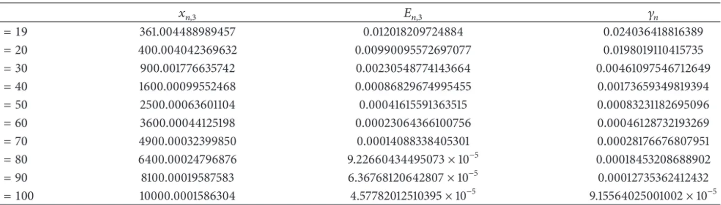
𝑥𝑛,3 𝐸𝑛,3 𝛾𝑛 𝑛 = 19 361.004488989457 0.012018209724884 0.024036418816389 𝑛 = 20 400.004042369632 0.00990095572697077 0.0198019110415735 𝑛 = 30 900.001776635742 0.00230548774143664 0.00461097546712649 𝑛 = 40 1600.00099552468 0.00086829674995455 0.00173659349819394 𝑛 = 50 2500.00063601104 0.00041615591363515 0.00083231182695096 𝑛 = 60 3600.00044125198 0.00023064366100756 0.00046128732193269 𝑛 = 70 4900.00032399850 0.00014088338405301 0.00028176676807951 𝑛 = 80 6400.00024796876 9.22660434495073× 10⁻⁵ 0.00018453208688902 𝑛 = 90 8100.00019587583 6.36768120642807× 10⁻⁵ 0.00012735362412432 𝑛 = 100 10000.0001586304 4.57782012510395× 10⁻⁵ 9.15564025001002× 10⁻⁵
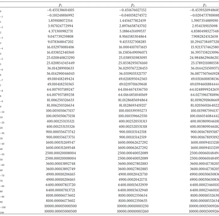
Table 4: Approximation of eigenvalues. 𝑝1 𝑝2 𝑝3 𝜆0 −0.455138604105 −0.451676027152 −0.4539320948685 𝜆−1 −0.110248816992 −0.040158274572 −0.0204737818081 𝜆1 1.859108072514 1.4456177812459 1.3907354889190 𝜆−2 3.917024772994 2.8976658743702 2.9541319115098 𝜆2 4.371300982731 5.1886431499537 4.8580498527548 𝜆−3 9.047739259808 8.9161585304864 7.9082824512658 𝜆3 9.078368847202 9.4153327308285 10.2941738497520 𝜆−4 16.032970081406 16.0004107071615 15.9213717462580 𝜆4 16.033832340360 16.1585649096071 16.3957158213096 𝜆−5 25.020840823290 25.0389311983095 24.9848629686203 𝜆5 25.020854345449 25.0538295076160 25.1789211080558 𝜆−6 36.014289910633 36.0293767228453 36.0144251509371 𝜆6 36.014290046045 36.0319035321757 36.0877507661928 𝜆−7 49.010418249424 49.0218195042565 49.0311600838136 𝜆7 49.010418250365 49.0219701639618 49.0394601884444 𝜆−8 64.007937189247 64.0164674336750 64.0248999242659 𝜆8 64.007937189258 64.0164851040169 64.0271961781896 𝜆−9 81.006250326633 81.0128685694864 81.0198291868669 𝜆9 81.006250326634 81.0128693419217 81.0203601164022 𝜆−10 100.005050675157 100.010339593273 100.015987594137 𝜆10 100.005050675158 100.010339662550 100.016034084442 𝜆−20 400.001253135321 400.002520531313 400.003809046181 𝜆20 400.001253135326 400.002520531318 400.003809046182 𝜆−30 900.000556173742 900.001115142518 900.001678193187 𝜆30 900.000556173751 900.001115142519 900.001678193192 𝜆−40 1600.00031269547 1600.00062627292 1600.00094113218 𝜆40 1600.00031269548 1600.00062627292 1600.00094113219 𝜆−50 2500.00020008004 2500.00040052089 2500.00060148494 𝜆50 2500.00020008004 2500.00040052089 2500.00060148495 𝜆−60 3600.00013892748 3600.00027802883 3600.00041738205 𝜆60 3600.00013892749 3600.00027802885 3600.00041738205 𝜆−70 4900.00010206165 4900.00020421710 4900.00030650836 𝜆70 4900.00010206165 4900.00020421711 4900.00030650836 𝜆−80 6400.00007813720 6400.00015632939 6400.00023460110 𝜆80 6400.00007813721 6400.00015632940 6400.00023460110 𝜆−90 8100.00006173602 8100.00012350634 8100.00018532630 𝜆90 8100.00006173602 8100.00012350635 8100.00018532634 𝜆−100 10000.00005000500 10000.00010003250 10000.00015009260 𝜆100 10000.00005000500 10000.00010003260 10000.00015009260
that is,𝑞𝑛 = 𝑞−𝑛= 1 for 1 ≤ 𝑛 ≤ 𝑠 and 𝑞𝑛= 𝑞−𝑛= 0 for 𝑛 > 𝑠, where𝑞𝑛is defined in (9). Note that the operator𝑇(𝑝1) is a famous Mathieu operator. By (19) and (108),𝑄 = 1 and 𝑀 = 𝑐. For 𝑠 = 1, 2,3 the constant 𝑀 or 𝑐 has the values of 2, 4, 6, respectively. The fixed point approximations𝑥𝑛,3determined in (55), where𝑓(𝑥) is defined by (40) with𝑚 = 3, of the eigenvalues𝜆±𝑛of the operators𝑇(𝑝𝑠) for 𝑠 = 1, 2, 3 are given in Tables1,2, and3, respectively. Moreover, the estimations of the error𝐸𝑛,3= |𝜆±𝑛− 𝑥𝑛,3| (see (64)) and the length𝛾𝑛of the𝑛th gap (see (45)) are also given in Tables1,2, and3.
The method of Section 3 gives high precision results for the calculation of the small eigenvalues. Let us illus-trate it by using formula (98) for the first 201 eigenvalues 𝜆0,𝜆−1,𝜆1,𝜆−2,𝜆2, . . . , 𝜆−100,𝜆100 of the operators 𝑇(𝑝𝑠) for
𝑠 = 1, 2, 3. It means that the number 𝑙 in (98) is 100 (see the first sentence of Section 3). To find an approximation with error of order 10−18 for the eigenvalues of 𝑇(𝑝1) we take 𝑟 = 5. Therefore for the potential 𝑝𝑠(𝑥), where 𝑠 = 1, 2, 3, the number 𝑆 is 𝑙 + 2𝑟𝑠 = 100 + 10𝑠 and the number of equations in (65) is 2𝑆 + 1 = 200 + 20𝑠 + 1. The matrices of (65) corresponding to the potentials 𝑝1(𝑥), 𝑝2(𝑥), 𝑝3(𝑥) and denoted by 𝐴1, 𝐴2, 𝐴3 are of order
221, 241, and 261, respectively. The approximate eigenvalues 𝜇0, 𝜇−1, 𝜇1, 𝜇−2, 𝜇2, . . . , 𝜇−100, 𝜇100 of the matrices𝐴1, 𝐴2, 𝐴3 are given inTable 4. By (98) the eigenvalues𝜇𝑛are very close to the eigenvalues𝜆𝑛of the operator𝑇(𝑝𝑠). One can readily see from (98) that the approximation|𝜆𝑛− 𝜇𝑛| of 𝜆𝑛 by the eigenvalues𝜇𝑛is arbitrary small if𝑟 is a large number and 𝑐 is
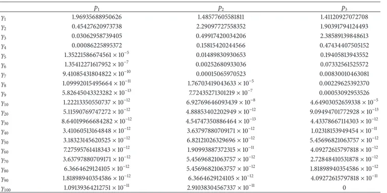
Table 5: Approximation of the lengths of the gaps. 𝑝1 𝑝2 𝑝3 𝛾1 1.96935688950626 1.48577605581811 1.41120927072708 𝛾2 0.45427620973738 2.29097727558352 1.90391794124493 𝛾3 0.03062958739405 0.49917420034206 2.38589139848613 𝛾4 0.00086225895372 0.15815420244566 0.47434407505152 𝛾5 1.35221586674561× 10⁻⁵ 0.01489830930653 0.19405813943552 𝛾6 1.35412271617952× 10⁻⁷ 0.00252680933036 0.07332561525572 𝛾7 9.41085431804822× 10⁻¹⁰ 0.00015065970523 0.00830010463081 𝛾8 1.09992015495664× 10⁻¹¹ 1.76703419043633× 10⁻⁵ 0.00229625392370 𝛾9 5.82645043323282× 10⁻¹³ 7.72435271301219× 10⁻⁷ 0.00053092953526 𝛾10 1.22213350550737× 10⁻¹² 6.92769646093439× 10⁻⁸ 4.64903052659338× 10⁻⁵ 𝛾20 5.11590769747272× 10⁻¹² 4.88853402202949× 10⁻¹² 9.09494701772928× 10⁻¹³ 𝛾30 8.64019966684282× 10⁻¹² 4.54747350886464× 10⁻¹³ 4.43378667114303× 10⁻¹² 𝛾40 3.41060513164848× 10⁻¹² 3.63797880709171× 10⁻¹² 1.02318153949454× 10⁻¹¹ 𝛾50 3.18323145620525× 10⁻¹² 6.82121026329696× 10⁻¹² 5.45696821063757× 10⁻¹² 𝛾60 7.27595761418343× 10⁻¹² 1.90993887372315× 10⁻¹¹ 4.09272615797818× 10⁻¹² 𝛾70 3.63797880709171× 10⁻¹² 5.45696821063757× 10⁻¹² 2.72848410531878× 10⁻¹² 𝛾80 6.3664629124105× 10⁻¹² 5.45696821063757× 10⁻¹² 1.81898940354586× 10⁻¹² 𝛾90 1.81898940354586× 10⁻¹² 6.3664629124105× 10⁻¹² 4.09272615797818× 10⁻¹¹ 𝛾100 1.09139364212751× 10⁻¹¹ 2.91038304567337× 10⁻¹¹ 0
a small number. If the potential𝑞 is smooth function, then the number𝑐 is a small number (see (13) and (19)), and hence (98) gives better approximations for smooth potentials. Moreover if𝑠 is a small number, that is, the number of summand of 𝑝𝑠 (see (108)) is small, then we can choose𝑟 so that the order of the matrix𝐴𝑠is not a large number while the approximation (98) is a very small number. By formula (98)|𝜆𝑛− 𝜇𝑛|, where 𝑛 = 0, ±1, ±2, . . . , ±100, for the potentials 𝑝1(𝑥), 𝑝2(𝑥), and 𝑝3(𝑥) is not greater than
8 × 110 × 212 (200)11 = 11 62510−17, 8 × 120 × 2 × 412 (200)11 = 3 1907 348 632 812 500, 8 × 130 × 3 × 612 (200)11 = 20 726 199 62 500 000 000 000 000 000, (109)
respectively. Thus inSection 3there are the following obser-vations to be considered. Instead of the matrices of order 201 investigating a little big matrices, namely, matrices of order 221, 241, and 261, we find an approximation of order10−18, 10−15, and10−12for the first201 eigenvalues of 𝑇(𝑝1), 𝑇(𝑝2), and 𝑇(𝑝3), respectively. Moreover this approach is applicable for the trigonometric polynomial potentials and for the sufficiently differentiable periodic potentials.
The estimations of the lengths𝛾1, 𝛾2, . . . , 𝛾100of the gaps are given in Table 5. It is known that [12] for large𝑛 the behavior of 𝛾𝑛 is sensitive to smoothness properties of the potential𝑞. If 𝑞 is 𝑚 times differentiable, then 𝛾𝑛 = 𝑂(𝑛−𝑚). If𝑞 is analytic function, then 𝛾𝑛 = 𝑂(𝑒−𝑎𝑛) for some positive 𝑎. For the Mathieu operator 𝑇(𝑝1) the following asymptotic formula holds: 𝛾𝑛 = 𝑂(4𝑛/((𝑛 − 1)!)2). Thus for large 𝑛
the length𝛾𝑛of the𝑛th gap is a very small number.Table 5 confirms this result for large𝑛 (see 𝛾𝑛for𝑛 ≥ 10). Moreover Table 5 shows that these results continue to hold for 𝑛 > 5. Since for the small values of 𝑛 (𝑛 ≤ 5) the asymptotic formulas do not give any information, we cannot compare the theoretical results with the results inTable 5. Note that in Tables4and5the eigenvalues and the lengths of the gaps are computed using Matlab. InTable 4this program transects to 14 figures, because this accuracy is acceptable for estimations of the eigenvalues. However, we compute the lengths of the gaps without transaction, since (as it is noted above) for large 𝑛 the theoretical results give the estimations of 𝛾𝑛with very high accuracy.
It is natural and well known that for large eigenvalues the asymptotic method gives us approximations with smaller errors. Since the method of Section 3gives high precision results for the small eigenvalues and gaps (see Tables4and 5), the comparison of the Tables1–5, where we estimate the eigenvalues and gaps by the methods of Sections2 and 3, respectively, for the potential (108), shows that the results of the asymptotic method given in Tables1–3are not precise for the small eigenvalues.
References
[1] M. S. P. Eastham, The Spectral Theory of Periodic Differential
Equations, Scottish Acedemic Press, Edinburg, UK, 1973.
[2] J. P¨oschel and E. Trubowitz, Inverse Spectral Theory, Academic Press, Boston, Mass, USA, 1987.
[3] A. L. Andrew, “Correction of finite element eigenvalues for problems with natural or periodic boundary conditions,” BIT, vol. 28, no. 2, pp. 254–269, 1988.
[4] A. L. Andrew, “Correction of finite difference eigenvalues of periodic Sturm-Liouville problems,” Journal of Australian
Mathematical Society B, vol. 30, no. 4, pp. 460–469, 1989.
[5] D. J. Condon, “Corrected finite difference eigenvalues of peri-odic Sturm-Liouville problems,” Applied Numerical
Mathemat-ics, vol. 30, no. 4, pp. 393–401, 1999.
[6] G. Vanden Berghe, M. Van Daele, and H. De Meyer, “A mod-ified difference scheme for periodic and semiperiodic Sturm-Liouville problems,” Applied Numerical Mathematics, vol. 18, no. 1–3, pp. 69–78, 1995.
[7] X. Ji and Y. S. Wong, “Pr¨ufer method for periodic and semi-periodic sturm-liouville eigenvalue problems,” International
Journal of Computer Mathematics, vol. 39, pp. 109–123, 1991.
[8] Y. S. Wong and X. Z. Ji, “On shooting algorithm for Sturm-Liouville eigenvalue problems with periodic and semi-periodic boundary conditions,” Applied Mathematics and Computation, vol. 51, no. 2-3, pp. 87–104, 1992.
[9] X. Z. Ji, “On a shooting algorithm for Sturm-Liouville eigen-value problems with periodic and semi-periodic boundary conditions,” Journal of Computational Physics, vol. 111, no. 1, pp. 74–80, 1994.
[10] V. Malathi, M. B. Suleiman, and B. B. Taib, “Computing eigen-values of periodic Sturm-Liouville problems using shooting technique and direct integration method,” International Journal
of Computer Mathematics, vol. 68, no. 1-2, pp. 119–132, 1998.
[11] O. A. Veliev and M. T. Duman, “The spectral expansion for a nonself-adjoint Hill operator with a locally integrable potential,”
Journal of Mathematical Analysis and Applications, vol. 265, no.
1, pp. 76–90, 2002.
[12] J. Avron and B. Simon, “The asymptotics of the gap in the Mathieu equation,” Annals of Physics, vol. 134, no. 1, pp. 76–84, 1981.
Submit your manuscripts at
http://www.hindawi.com
Hindawi Publishing Corporation
http://www.hindawi.com Volume 2014
Mathematics
Journal ofHindawi Publishing Corporation
http://www.hindawi.com Volume 2014
Mathematical Problems in Engineering
Hindawi Publishing Corporation http://www.hindawi.com
Differential Equations International Journal of
Volume 2014
Hindawi Publishing Corporation
http://www.hindawi.com Volume 2014 Hindawi Publishing Corporationhttp://www.hindawi.com Volume 2014
Hindawi Publishing Corporation
http://www.hindawi.com Volume 2014 Mathematical PhysicsAdvances in
Complex Analysis
Journal ofHindawi Publishing Corporation
http://www.hindawi.com Volume 2014
Optimization
Journal of Hindawi Publishing Corporationhttp://www.hindawi.com Volume 2014
Combinatorics
Hindawi Publishing Corporation
http://www.hindawi.com Volume 2014 International Journal of
Hindawi Publishing Corporation
http://www.hindawi.com Volume 2014
Journal of
Hindawi Publishing Corporation
http://www.hindawi.com Volume 2014
Function Spaces
Abstract and Applied Analysis Hindawi Publishing Corporation
http://www.hindawi.com Volume 2014 International Journal of Mathematics and Mathematical Sciences
Hindawi Publishing Corporation http://www.hindawi.com Volume 2014
The Scientific
World Journal
Hindawi Publishing Corporation
http://www.hindawi.com Volume 2014
Hindawi Publishing Corporation
http://www.hindawi.com Volume 2014
Discrete Dynamics in Nature and Society Hindawi Publishing Corporation
http://www.hindawi.com Volume 2014
Hindawi Publishing Corporation
http://www.hindawi.com Volume 2014
Discrete Mathematics
Journal ofHindawi Publishing Corporation
http://www.hindawi.com Volume 2014 Hindawi Publishing Corporationhttp://www.hindawi.com Volume 2014