Provisioning Virtual Private Networks under Traffic
Uncertainty
A. Altın
Department of Industrial Engineering, Bilkent University, Ankara, Turkey E. Amaldi
Dipartimento di Elettronica e Informazione, Politecnico di Milano, Italy P. Belotti
Dipartimento di Elettronica e Informazione, Politecnico di Milano, Italy M. C¸ . Pınar
Department of Industrial Engineering, Bilkent University, Ankara, Turkey
We investigate a network design problem under traffic uncertainty that arises when provisioning Virtual Private Networks (VPNs): given a set of terminals that must communicate with one another, and a set of possible traffic matrices, sufficient capacity has to be reserved on the links of the large underlying public network to support all possible traffic matrices while minimizing the total reservation cost. The problem admits several ver-sions depending on the desired topology of the reserved links, and the nature of the traffic data uncertainty. We present compact linear mixed-integer programming for-mulations for the problem with the classical hose traffic model and for a less conservative robust variant relying on the traffic statistics that are often available. These flow-based formulations allow us to solve optimally me-dium-to-large instances with commercial MIP solvers. We also propose a combined branch-and-price and cut-ting-plane algorithm to tackle larger instances. Compu-tational results obtained for several classes of instances are reported and discussed.© 2006 Wiley Periodicals, Inc.
NETWORKS, Vol. 49(1), 100 –115 2007
Keywords: virtual private networks; network design; traffic uncertainty; robust optimization; mixed-integer linear programs; branch and price; cutting planes
1. INTRODUCTION
Virtual Private Networks (VPNs) are network services built over an existing public network to provide quality of service, flexibility, and security while saving costs through
link multiplexing. They use encryption and tunneling to link branch offices to an enterprise network, or to extend orga-nizations’ existing computing infrastructure to include part-ners, suppliers, and customers [14]. The use of public net-works reduces operational costs due to economies of scale while ensuring a wider area accessibility and communica-tion security through encrypcommunica-tion. Flexibility and cost effec-tiveness have turned VPN solutions into a billion dollar industry.
In this article we address a network design problem that arises when provisioning VPNs. Given a set of terminals that must communicate with one another and a set of pos-sible traffic patterns, sufficient capacity has to be reserved on the links of the large underlying public network to support all possible traffic patterns while minimizing cost. The solution of this resource management problem clearly depends on the possible traffic patterns and the constraints on the topology of the reserved links.
In traditional network design problems, it is assumed that a traffic matrix, that is, a set of demands for all origin– destination pairs, can be reliably estimated. Because a VPN service customer has in general no precise information about the expected traffic between the terminals to be con-nected, a collection of possible traffic matrices have to be simultaneously considered. In [7] a flexible model referred to as the hose model was proposed to specify the bandwidth requirements of a single VPN. In this hose model, the set of
valid traffic matrices is defined by imposing, for each
ter-minal t, an upper bound on the total outgoing traffic from t (toward the other terminals) and an upper bound on the total entering traffic in t (from the other terminals).
The underlying network over which a VPN has to be provisioned is represented by an undirected graph G⫽ (V,
E). Each edge e in E, also denoted by {i, j} to emphasize
the two end-nodes i, j in V, has a per-unit nonnegative reservation cost cij. Let Q債 V denote the set of terminals
Received September 2004; accepted May 2006
Correspondence to: E. Amaldi; e-mail: [email protected]
Contract grant sponsor: TUBITAK, The Scientific and Technological Re-search Institute of Turkey; contract grant number: MISAG-CNR-1 Contract grant sponsor: CNR, Consiglio Nazionale delle Ricerche, Italy; contract grant number: MISAG-CNR-1
DOI 10.1002/net.20145
Published online in Wiley InterScience (www.interscience.wiley.com).
that need to communicate with one another. For each or-dered pair of terminals (s, t), with s, t僆 Q, the nonnega-tive dstrepresents the amount of traffic that has to be routed
from s to t. We assume that dss ⫽ 0 for every terminal s
and denote by S the set of all ordered pairs of distinct terminals, namely S ⫽ {(s, t) 僆 Q ⫻ Q : s ⫽ t}. In the hose model, two nonnegative bounds bs⫹and bs⫺ are
spec-ified for each terminal s in Q, and the traffic demands dstare
assumed to be nonnegative values that belong to the uncer-tainty set UAsymGdefined by the following inequalities:
冘
t:t⫽s dstⱕ bs⫹,冘
t:t⫽s dtsⱕ bs⫺ ᭙ s 僆 Q (1) dstⱖ 0 ᭙ 共s, t兲 僆 S. (2)Throughout this article we make the realistic assumption that traffic is unsplittable, that is, for each demand pair (s,
t) 僆 S the traffic demand dst is routed along a single path
from s to t. (Although the case where each traffic demand can be arbitrarily split and routed along several paths is considered among others in [8], multipath routing is cur-rently hardly implementable in VPNs because packets re-lated to a single flow may arrive out of sequence and thus cause critical problems at the Transfer Control Protocol, TCP, level.) Provisioning a VPN then consists of reserving capacity on the edges and selecting a single routing path for each demand pair to support all valid traffic matrices while minimizing the total reservation cost. In the VPN provision-ing problems considered in the present article, no assump-tion is made on the integrality of demand values even if the bounds bs⫹and bs⫺are integral. In other words, the resulting
design should support integral as well as nonintegral traffic demand matrices from the uncertainty polyhedron (1)–(2). Therefore, the network design problem of the present arti-cle, which has a multicommodity flow structure, is both continuous and discrete in nature because fractional amounts of capacity can be reserved on the links while demands must be routed along single paths.
If no particular constraint is imposed on the topology of the reserved network (union of all edges with a strictly positive capacity reservation), the VPN provisioning prob-lem with the hose traffic model is called Asym-G. The version in which the reserved network is required to be a tree is referred to as Asym-T.
The symmetric versions, where a threshold bs is given
for the sum of incoming and outgoing traffic for all termi-nals s 僆 Q, are referred to as Sym-G and Sym-T, respec-tively. These assumptions imply that the traffic demands are elements of the set USymGdefined as follows:
冘
t:共s,t兲僆S dst⫹冘
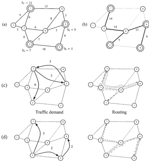
t:共t,s兲僆S dtsⱕ bs ᭙ s 僆 Q (3) dstⱖ 0 ᭙ 共s, t兲 僆 S, (4)with upper bounds on the cumulative entering and outgoing traffic. Figure 1 illustrates an instance of Sym-G, the corre-sponding optimal solution, and the routing of two traffic matrices within USymGwith the related routing.
To the best of our knowledge, the state of the art on the computational complexity of these variants can be summa-rized as follows:
● Sym-T can be solved in polynomial time by shortest path
computations [10];
● Asym-T is strongly NP-hard, and does not admit a
poly-nomial time approximation scheme, unless P⫽ NP [10], and the best known approximation algorithm is guaran-teed to yield a VPN whose total reservation cost is at most 9.002 times larger than that of a minimum cost VPN [17];
● Any optimal solution for Sym-T provides a 2-approxima-tion to Sym-G [10] but it is still open whether Sym-G is actually NP-hard;
● The best approximation algorithm for Asym-G has a 5.55 factor [11] but it is still open whether Asym-G is actually NP-hard.
In the present article we develop new, compact, linear mixed-integer programming (MIP) formulations for the
Asym-G and Sym-G variants of the VPN provisioning
prob-lem under the hose model of uncertainty (cf. Proposition 1). Although the computational complexity status of Asym-G is still open, medium-to-large instances of our models turn out to be solvable by the off-the-shelf mixed-integer optimizer Cplex 8.1 within short computing time.
Traffic uncertainty is a crucial feature in VPN provision-ing. Because the hose model makes very weak assumptions (only imposes upper bounds on the inflow and outflow of each terminal), it may lead to excessive capacity reserva-tion. This traffic model is a special case of the so-called
polyhedral model in which the set of valid matrices is
defined by an arbitrary polyhedron [4]. In principle, the polyhedral model allows us to focus on smaller subsets of traffic matrices than the hose model, but it is unclear how to actually define realistic polyhedra that would lead to less conservative VPN reservations.
From the application point of view, a service provider simultaneously provisions a number of VPNs for different customers over a certain time period and the service level agreements are renegotiated on a regular basis. Although the hose traffic model is adequate for new VPNs in the absence of precise traffic predictions, it is clearly overly conservative for VPNs that are already provisioned. Because service providers collect detailed terminal-to-terminal traffic statistics for each VPN, a less conservative traffic uncertainty model that exploits the available statistics is needed. Therefore, we investigate a less conservative robust variant of the problem, which exploits the traffic statistics that are available for existing VPNs. In particular, a corresponding compact linear MIP formulation is presented (cf. Proposition 2) and the robust VPN provisioning problem is shown to be NP-hard (cf. Proposition 3).
In practice, service providers face an incremental reser-vation problem: while provisioning a given set of VPNs,
they receive a request for a new VPN or for changes to the set of terminals of an existing one. Because the additional capacity requirements for a single VPN are in general very small compared with the overall network capacity, it is reasonable from an application point of view to focus on the uncapacitated versions of the VPN provisioning problem (A. Capone, personal communication, 2003). Due to the absence of capacity constraints and the fractional capacity that can be reserved on each link of the backbone network, the incremental problem can then be decomposed into a sequence of single VPN provisioning problems with appro-priate traffic uncertainty models.
The rest of the article is organized as follows. In Section 2.1 we present compact flow-based linear MIP formulations for
Asym-G and Sym-G under the hose uncertainty model. In
Section 2.2 we investigate the less conservative robust variant of the VPN provisioning problem. For both hose uncertainty and robust uncertainty models we also discuss cutting planes for obtaining lower bounds. Finally, to close the discussion of the models, in Section 2.3 we give the path-based formulations more suitable for the exact solution method detailed in Section
3 where we describe a combined branch-and-price and cutting-plane algorithm to tackle larger instances of the three problem versions. Computational results obtained for several classes of instances are reported and discussed in Section 4. Section 5 contains some concluding remarks.
2. VPN PROVISIONING MODELS
2.1. VPN Provisioning Problem with the Hose Traffic Model
For new VPNs or existing ones in which at least a new terminal is added, demand statistics are not available or not reliable due to the lack of information about the traffic generated by the new terminals. The hose uncertainty model is then well suited for the demands involving at least a new terminal.
Consider the general variant Asym-G with asymmetric traffic matrices. The network cost, which depends on the capacity to be reserved so as to route all demands, has to be minimized. Because traffic is assumed to be unsplittable, FIG. 1. An instance of Sym-G. The network topology is given in (a) with edge capacity costs, terminal nodes 3, 5,
6, and 7 are emphasized and the upper bounds bsare indicated. An optimal solution is shown in (b) with edge capacities. Two sets of traffic demands within USymGare given in (c) and (d), with the related routing. For example,
each demand has to be routed along a single path from origin to destination.
2.1.1. From Constant Traffic Matrices to the Hose Model. Let us first consider the capacity reservation prob-lem aiming at minimizing cost while supporting a single traffic matrix D⫽ (dst)s,t僆Qand note that a straightforward minimum cost flow formulation can be solved in polyno-mial time. We define two classes of variables. For each edge {i, j}, the continuous variable xijrepresents the capacity to be reserved on {i, j}. Let A⫽ {(i, j) : {i, j} 僆 E} denote the underlying set of oriented arcs. For each oriented arc (i,
j)僆 A and oriented pair of terminals (s, t) 僆 S, the binary
variable yijstcorresponds to the flow on the oriented arc (i, j)
for the terminal pair (s, t)
yij st
⫽
再
1 if arc共i, j兲 is used to route demand dst0 otherwise.
This leads to the flow formulation:
min
冘
兵i, j其僆E cijxij (5) s.t.冘
j:兵i, j其僆E 共yij st⫺ y ji st兲 ⫽再
1 i⫽ s ⫺1 i ⫽ t 0 otherwise ᭙ i 僆 V, ᭙ 共s, t兲 僆 S (6)冘
共s,t兲僆S dst共 yij st⫹ y ji st兲 ⱕ x ij ᭙ 兵i, j其 僆 E (7) yij st 僆 兵0, 1其 ᭙ 共i, j兲 僆 A, ᭙ 共s, t兲 僆 S (8) xijⱖ 0 ᭙ 兵i, j其 僆 E, (9)where the objective function corresponds to the VPN res-ervation cost. Constraints (6) ensure demand satisfaction by imposing a unit flow between each oriented pair of termi-nals. For each edge {i, j} the corresponding constraint (7) guarantees that the capacity xij reserved on {i, j} is
suffi-cient to carry the total traffic flowing through it.
If all the demands dst are precisely known, (5)–(9) is a
linear mixed-integer program. Due to the nonnegativity of the costs cijand of all variables, constraints (7) are satisfied
as equalities in any optimal solution to (5)–(9). Therefore, the continuous variables xijcan be omitted and we have the
equivalent formulation: min
冘
兵i, j其僆E cij冘
共s,t兲僆S dst共yij st ⫹ yji st 兲 (10) s.t.冘
j:兵i, j其僆E 共yij st ⫺ yji st 兲 ⫽再
1 i⫽ s ⫺1 i ⫽ t 0 otherwise ᭙ i 僆 V, ᭙ 共s, t兲 僆 S (11) yij st僆 兵0, 1其 ᭙ 共i, j兲 僆 A, ᭙ 共s, t兲 僆 S (12) with only binary variables. Because there are no capacity constraints and fractional capacities can be reserved on the edges, the constraint matrix is totally unimodular and the problem is solvable in polynomial time [15].If the traffic matrix D is subject to the hose uncertainty model, a first formulation is obtained by requiring that capacity constraints (7) hold for all traffic matrices satisfy-ing constraints (1)–(2), or respectively (3)–(4). Thus, we obtain the following semi-infinite MIP formulation
min
冘
兵i, j其僆E cijxij (13) s.t.冘
j:兵i, j其僆E 共yij st⫺ y ji st兲 ⫽再
1 i⫽ s ⫺1 i ⫽ t 0 otherwise ᭙ i 僆 V, ᭙ 共s, t兲 僆 S (14)冘
共s,t兲僆S dst共 yij st⫹ y ji st兲ⱕ xij ᭙ D 僆 UAsymG共USymG兲, ᭙ 兵i, j其 僆 E (15)
yij
st僆 兵0, 1其 ᭙ 共i, j兲 僆 A, ᭙ 共s, t兲 僆 S
(16)
xijⱖ 0 ᭙ 兵i, j其 僆 E. (17)
Two previous works [4, 8] deal with the semi-infinite nature of the problem by dynamically generating a set of traffic matrices corresponding to vertices of the demand polyhedron. Solving the restricted problem yields values for the flow variables y˜ij
st
and the capacity variables x˜ij. Because
the resulting routing vector y˜ may be infeasible for the hose polyhedron defined by constraints (1)–(2), or by (3)–(4), a new vertex (traffic matrix) is sought by solving another linear program, where the y˜s and x˜s are considered as coefficients and the edge overload ¥(s,t)僆S dst( y˜ij
st ⫹ y˜ ji st
) ⫺ x˜ij is maximized over this polyhedron. If there exists a
valid traffic matrix (dˇst)s,t僆Q that is not supported by the
capacity x˜ijreserved on edge {i, j}, that is, if such overload
is positive, a new constraint (7) with coefficients dˇst is
added to the formulation. If no such traffic matrix is found for any edge {i, j}, the reserved capacities support all valid traffic matrices. Thus, these row-generation algorithms re-peatedly improve a dual bound until primal feasibility is reached. Although the focus is on critical demand values, 兩E兩 linear programs must be solved at each iteration. In the
special case of the hose model, these linear programs reduce to min-cost-flow problems, which yield an integral maxi-mum flow on each edge [4]. In [4], computational results are reported for a special class of instances with unbounded entering traffic in each terminal. In [8], the authors consider multiple-path routing and check the validity of a reservation vector over a demand polyhedron with integral vertices. To the best of our knowledge, this does not actually imply that such a reservation vector supports all valid traffic matrices with fractional demands when single-path routing is con-sidered. Examples where a reservation vector that is feasible for all valid integral traffic matrices does not support some valid fractional ones, can indeed be easily found.
2.1.2. A Compact Linear MIP Formulation for the Problem with Hose Model. Unlike in the above-men-tioned works, we simultaneously consider all demand con-straints and derive a compact linear MIP formulation that avoids the semi-infinite MIP formulation.
Proposition 1. The Asym-G problem (13)–(17) is equiv-alent to the following linear mixed-integer program:
min
冘
兵i, j其僆E cijxij (18) s.t.冘
j:兵i, j其僆E 共yij st⫺ y ji st兲 ⫽再
1 i⫽ s ⫺1 i ⫽ t 0 otherwise ᭙ i 僆 V, ᭙ 共s, t兲 僆 S (19)冘
s僆Q 共bs⫹ij s⫹⫹ b s ⫺ ij s⫺兲 ⱕ x ij ᭙ 兵i, j其 僆 E (20) ij s⫹⫹ ij t⫺ⱖ 共 y ij st ⫹ yji st 兲 ᭙ 兵i, j其 僆 E, ᭙ 共s, t兲 僆 S (21) yij st僆 兵0, 1其 ᭙ 共i, j兲 僆 A, ᭙ 共s, t兲 僆 S (22) ij s⫹, ij s⫺, x ijⱖ 0 ᭙ 兵i, j其 僆 E, ᭙ s 僆 Q. (23)Proof. Start from the semi-infinite flow formulation (13)–(17). Consider a single edge {i, j} and treat the y variables as parameters. The worst-case value for the ca-pacity xij to be reserved on edge {i, j} is obtained by
solving the following optimization problem:
xijⱖ max
冘
共s,t兲僆S dst共yij st⫹ y ji st兲 (24) 共ij s⫹兲冘
t⫽s dstⱕ bs⫹ ᭙ s 僆 Q (25) 共ij s⫺兲冘
t⫽s dtsⱕ bs⫺ ᭙ s 僆 Q (26) dstⱖ 0 ᭙ 共s, t兲 僆 S, (27)where thes are the corresponding dual variables. Because this linear program is feasible and bounded, we can apply a duality transformation similarly to [16] to obtain the equiv-alent formulation: xijⱖ min
冘
s僆Q 共bs⫹ij s⫹⫹ b s ⫺ ij s⫺兲 (28) ij s⫹⫹ ij t⫺ⱖ y ij st⫹ y ji st ᭙ 共s, t兲 僆 S (29) ij s⫹ ,ij s⫺ⱖ 0 ᭙ s 僆 Q. (30) By replacing constraints (24)–(27) with (28)–(30), we ob-tain a lower bound on the capacity that is required on edge {i, j}. This substitution immediately leads from (13)–(17) to the linear MIP formulation (18)–(23) after observing that the min in (28) can be omitted due to the nature of the objective function, which is a nonnegatively weighted sum of the variables xij, and the continuous nature of the xijvariables. ■
Analogously, for the Sym-G case we obtain a compact formulation with the same objective function (18), the flow conservation constraint (19), constraints (22), and
冘
s僆Q bsij s ⱕ xij ᭙ 兵i, j其 僆 E (31) ij s ⫹ij t ⱖ yij st ⫹ yji st ᭙ 兵i, j其 僆 E, ᭙ 共s, t兲 僆 S (32) ij s , xijⱖ 0 ᭙ 兵i, j其 僆 E, ᭙ s 僆 Q. (33)As we shall see in Section 4, tackling this compact linear MIP formulation with commercial solvers (e.g., Cplex 8.1) yields optimal solutions in reasonable time even for large-size instances.
2.1.3. Cutting Planes and Lower Bounds. Some valid inequalities can be easily derived for the formulations given in the preceding paragraphs. These inequalities are useful in cutting plane procedures for numerical solution of large instances as we shall see in Section 4.
Let us consider the flow formulation (18)–(23) of
Asym-G. For any subset of edges F 債 E, we use the
notation x(F) ⫽ ¥{i, j}僆Fxijand, similarly, for any subset
of arcs F⬘ 債 A the notation yst(F⬘) ⫽ ¥(i, j)僆F⬘yij st
. For any subset of nodes W 傺 V, the cut␦(W) is the set of edges with only one end-node in W, that is,␦(W) ⫽ {{i, j} 僆 E : i僆 W, j ⰻ W}. For any subset W 傺 V, the directed cut ␦⬘(W) is the set of arcs with the tail in W and the head in
VW.
Given any subset W傺 V, if there exists a nonempty set of terminal pairs S⬘ ⫽ {(s, t) 僆 S : s 僆 W, t 僆 VW}, then for each one of these terminal pairs (s, t) at least one flow variable associated with an arc of the directed cut ␦⬘(W) must be nonzero, that is,
yst共␦⬘共W兲兲 ⱖ 1.
(34) From (21) we obtain the following family of inequalities:
冘
共i, j兲僆␦⬘共W兲 共ij s⫹⫹ ij t⫺兲 ⱖ 1 ᭙ 共s, t兲 僆 S : 兩兵s, t其 艚 W兩 ⫽ 1 (35) that only involve variables and that are satisfied by any feasible solution of Asym-G.Consider now the capacity x[␦(W)] needed across a cut ␦(W) to support the demands between all terminal pairs whose endpoints are on different shores. A lower bound is as follows:
x共␦共W兲兲 ⱖ
冘
共s,t兲僆S:兩兵s,t其艚W兩⫽1
dst. (36)
Given the traffic uncertainty, the right-hand side of (36) is not known a priori and x[␦(W)] has to be large enough in the worst case scenario. Because the maximum traffic across a cut␦[W)], denoted by d[␦(W)], amounts to
max
再
冘
共s,t兲僆S:兩兵s,t其艚W兩⫽1 dst:冘
t:t⫽s dtsⱕ bs⫺ ᭙ s 僆 Q,冘
t:t⫽s dst ⱕ bs⫹ ᭙ s 僆 Q, dstⱖ 0 ᭙ 共s, t兲 僆 S冎
,any feasible solution of Asym-G must satisfy x[␦(W)] ⱖ
d[␦(W)]. As xijis defined in constraints (20), we can write
equivalently:
冘
兵i, j其僆␦共W兲s冘
僆Q 共bs⫹ij s⫹⫹ b s ⫺ ij t⫺兲 ⱖ d关␦共W兲兴. (37)The demand cut-set inequalities (35) and the capacity
cut-set inequalities (37) express two necessary conditions
for supporting all valid traffic matrices.
Inequalities (35) and (37) are not violated by a solution of the linear relaxation of the formulation (18)–(23), as they are implied by the flow conservation constraints (19). How-ever, a cut formulation including only the variables and a subset of these inequalities provides a lower bound on
Asym-G. As for (37), we may get rid of the x variables and
express the objective function in terms of the variables only:
冘
兵i, j其僆E cij冘
共s,t兲僆S 共bs⫹ij s⫹⫹ b s ⫺ ij t⫺兲. (38)The goal is then to minimize (38) subject to inequalities (35) and (37). A cutting-plane procedure for obtaining a lower bound on the optimal value of Asym-G takes a small initial set of such inequalities and repeatedly adds violated cuts identified through efficient separation procedures. Although separating inequalities (35) requires solving a maximum-flow problem, and hence is easy, separating inequalities (37) can be shown to be NP-hard.
In the present article we derive dual (lower) bounds on the optimal value by using inequalities (35). Consider G ⫽ (V, E) and the set of values (bs⫹, bs⫺), @s 僆 Q. Let ⌬
denote a subset of all possible triplets {s, t,␦(W)}, where
W 傺 V and 兩{s, t} 艚 W兩 ⫽ 1. A lower bound is given by
the following linear program: 共Pdual兲 min
冘
兵i, j其僆E cij冘
共s,t兲僆S 共bs⫹ij s⫹⫹ b s ⫺ ij t⫺兲 s.t.冘
共i, j兲僆␦⬘共W兲 共ij s⫹⫹ ij t⫺兲 ⱖ 1 ᭙ 共s, t, W兲 僆 ⌬.Because this problem does not involve the y variables, it is quickly solved for a reasonable number of inequalities.
Inequalities (35) and (37) are easily adapted to Sym-G. From (32) and (34) we obtain the following two families of valid inequalities:
冘
共i, j兲僆␦⬘共W兲 共ij s⫹ ij t兲 ⱖ 1 ᭙ W 傺 V, ᭙ 共s, t兲 僆 S : 兩兵s, t其 艚 W兩 ⫽ 1冘
兵i, j其僆␦共W兲s冘
僆Q bsij sⱖ d共␦共W兲兲 ᭙ W 傺 V.2.2. Robust VPN Provisioning Problem
Because detailed traffic statistics (reliable average and standard deviation estimates of terminal-to-terminal traffic) are available for existing VPNs, we consider a variant of the VPN provisioning problem that exploits this additional in-formation. Unlike the hose model, where bounds are im-posed on the aggregated traffic through each terminal, we adopt a less conservative traffic uncertainty model and consider each demand dst individually. However, our
as-sumptions regarding the valid traffic matrices are very mild: we just assume that we know the range of values that each demand dstcan take. Specifically, for each pair of terminals s, t 僆 Q, the demand dst is assumed to take values in an
interval [d⬘st⫺ dˆst, d⬘st⫹ dˆst], where dˆst僆 [0, d⬘st] denotes
the positive deviation from the nominal value d⬘st. It is worth
emphasizing that we do not make any assumptions concern-ing the distribution of the traffic demands within the
corre-sponding intervals and concerning the way different de-mands dst may be interrelated.
For nonnegative deviations dˆst, the robust VPN
provi-sioning problem in which the demands are subject to the above interval uncertainty can be formulated as the follow-ing binary integer program:
min
冘
兵i, j其僆E cij冘
共s,t兲僆S 共d⬘st⫹ dˆst兲共yij st ⫹ yji st 兲 (39) s.t.冘
j:兵i, j其僆E 共yij st ⫺ yji st 兲 ⫽再
1 i⫽ s ⫺1 i ⫽ t 0 otherwise ᭙ i 僆 V, ᭙ 共s, t兲 僆 S (40) yij st 僆 兵0, 1其 ᭙ 共i, j兲 僆 A, ᭙ 共s, t兲 僆 S. (41) As for the nominal problem (10)–(12) corresponding to the nominal traffic matrix D⬘ ⫽ (d⬘st)s,t僆Q, this robust versioncan be solved in polynomial time.
Because it may be overly pessimistic to assume that all demands simultaneously vary within the corresponding un-certainty intervals so as to adversely affect the solution, we consider a positive integer parameter ⌫, 1 ⱕ ⌫ ⱕ 兩S兩, which allows us to adjust the tradeoff between the VPN robustness and its degree of conservatism as in the general approach for robust discrete optimization problems under data uncertainty proposed in [5, 6]. Whereas minimum and maximum values for point-to-point demand can be obtained through repeated measurements over time, it is difficult to predict when a demand is at its maximum. Although in principle we cannot exclude the possibility that all demands take their peak values simultaneously, traffic statistics show that, in general, peaks in the demand values are reached at different times. It is then reasonable to limit the conserva-tiveness of the model by adopting a robust approach a` la Bertsimas and Sim [5, 6] and by assuming that at any point in time at most⌫ of the demand values simultaneously take their worst-case values. In the VPN provisioning setting, the parameter⌫ can be interpreted as the margin on the risk that the operator is willing to take for not satisfying the customer requirements over a given period of time.
To avoid overdimensioned VPNs, we minimize the max-imum reservation cost while protecting us against the ex-treme behavior of at most⌫ of the demands. More precisely, we consider the following robust VPN provisioning prob-lem: min
冘
兵i, j其僆E cijxij (42) s.t.冘
j:兵i, j其僆E 共yij st ⫺ yji st 兲 ⫽再
1 i⫽ s ⫺1 i ⫽ t 0 otherwise ᭙ i 僆 V, ᭙ 共s, t兲 僆 S (43)冘
共s,t兲僆S d⬘st共 yij st ⫹ yji st 兲 ⫹ max兵S˜ : S˜ 債S,兩S˜ 兩ⱕ⌫其冘
共s,t兲僆S˜ dˆst共yij st ⫹ yji st 兲 ⱕ xij ᭙ 兵i, j其 僆 E (44) yij st僆 兵0, 1其 ᭙ 共i, j兲 僆 A, ᭙ 共s, t兲 僆 S (45) xijⱖ 0 ᭙ 兵i, j其 僆 E, (46)where S˜ denotes a subset of S of cardinality at most⌫. We refer to this robust variant of the problem as Rob-G. It is worth pointing out that the general probabilistic guarantees derived for the extreme behavior of more than⌫ parameters in [5] are also valid in our case. We also note that choosing ⌫ equal to the cardinality of S is equivalent to setting all demand values at their upper bounds, which yields the problem (39)–(41).
As for Sym-G and Asym-G, this robust variant of the VPN provisioning problem admits a compact linear MIP formulation. The following result can be viewed as a special case of the first theorem in [5] for general discrete optimi-zation problems.
Proposition 2. The robust VPN provisioning problem
(42)–(46) has the following equivalent linear mixed-integer
programming formulation: min
冘
兵i, j其僆E cijxij (47) s.t.冘
j:兵i, j其僆E 共yij st⫺ y ji st兲 ⫽再
1 i⫽ s ⫺1 i ⫽ t 0 otherwise ᭙ i 僆 V, ᭙ 共s, t兲 僆 S (48)冘
共s,t兲僆S d⬘st共 yij st⫹ y ij st兲 ⫹ ⌫ ij 0⫹冘
共s,t兲僆S ij stⱕ x ij ᭙ 兵i, j其 僆 E (49) ij 0⫹ ij stⱖ dˆ st共 yij st⫹ y ji st兲 ᭙ 兵i, j其 僆 E, ᭙ 共s, t兲 僆 S (50) yij st僆 兵0, 1其 ᭙ 共i, j兲 僆 A, ᭙ 共s, t兲 僆 S (51) ij 0 ,ij st , xijⱖ 0 ᭙ 兵i, j其 僆 E, ᭙ 共s, t兲 僆 S. (52) Proof. As in [5, 6], we first consider the constraints whose parameters are subject to uncertainty, namely con-straints (44). Given a vector y 僆 {0, 1}兩A兩⫻兩S兩, for each {i,j} 僆 E the problem max 兵S˜ : S˜債S,兩S˜兩ⱕ⌫其共s,t兲僆S˜
冘
dˆst共yij st ⫹ yji st 兲 (53)is equivalent to max
冘
共s,t兲僆S ␣stdˆst共yij st⫹ y ji st兲 (54) s.t.冘
共s,t兲僆S ␣stⱕ ⌫ (55) ␣st僆 兵0, 1其 ᭙ 共s, t兲 僆 S. (56)The key observation here is that the above problem, viewed as a linear program by relaxing the integrality of␣st
vari-ables, always has a binary optimal solution as it is a simple knapsack. Therefore, it can be replaced with
max
冘
共s,t兲僆S ␣stdˆst共yij st ⫹ yji st 兲 (57) s.t.冘
共s,t兲僆S ␣stⱕ ⌫ (58) 0ⱕ␣stⱕ 1 ᭙ 共s, t兲 僆 S, (59)which admits the following dual: min⌫ij 0⫹
冘
共s,t兲僆S ij st (60) s.t.ij 0⫹ ij stⱖ dˆ st共yij st⫹ y ji st兲 ᭙ 兵i, j其 僆 E, ᭙ 共s, t兲 僆 S (61) ij 0 ,ij stⱖ 0 ᭙ 兵i, j其 僆 E, ᭙ 共s, t兲 僆 S. (62) By strong duality this dual is feasible and bounded, and has the same optimal objective function value as the primal problem (54)–(56). Substituting (60)–(62) in (42)–(46)yields (47)–(52). ■
Unlike the robust discrete optimization problems with 0 –1 variables considered in [5], there is unfortunately strong evidence that the robust VPN provisioning problem is substantially harder to solve than the associated nominal problem, that is (39)–(41) with dˆst⫽ 0 for all (s, t) 僆 S,
which can be solved in polynomial time.
Proposition 3. The robust VPN provisioning problem
(42)–(46) is NP-hard.
Proof. We proceed by polynomial time reduction from the following version of the Satisfiability problem.
3-SAT: Given a set of m clauses C1, . . . , Cm in n
Boolean variables x1, . . . , xn and their complements x1, . . . , xn with exactly 3 literals per clause, does there
exist a truth assignment for the variables that satisfies all the clauses?
Because each clause is a disjunction of its literals, such a truth assignment must make true at least one literal per clause. The 3-SAT problem is known to be NP-complete even when restricted to instances in which each Boolean variable xj occurs (as xj or xj) in at most five clauses [9].
The construction is similar to the one used to establish that it is NP-complete to decide whether in a given graph k distinct pairs of nodes can be connected with k edge-disjoint paths.
For any given instance of 3-SAT where each variable occurs in at most five clauses, we will construct a special instance of the robust VPN provisioning problem, defined by a graph G ⫽ (V, E) with cij⫽ 1 for all {i, j} 僆 E, a
set of terminals Q 債 V, appropriate nominal demands and deviations between each pair of terminals and⌫ ⫽ 1. We will then verify that the former instance of 3-SAT is satis-fiable if and only if the latter instance admits a robust VPN of total cost at most 11n ⫹ 2m.
Consider an arbitrary instance of 3-SAT in which each Boolean variable occurs in at most five clauses. For each variable xjin this instance, we consider two terminals sjand tjin Q connected by two separate parallel paths
correspond-ing, respectively, to the variable xj and its complement xj.
Each one of these (sj, tj)-paths consists of 11 edges and has
10 intermediate nodes. For each clause Ci, we consider two
other terminals vi and wiin Q connected by three separate
parallel paths that correspond to the three literals in the clause. Each one of these (vi, wi)-paths consists of three
edges and has two intermediate nodes. The paths associated with the pairs of terminals (sj, tj), 1ⱕ j ⱕ n, and (vi, wi),
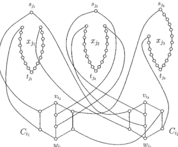
1 ⱕ i ⱕ m, must intersect in the appropriate way. For example, if the 3-SAT instance contains a first clause Ci1 with the literals xj1, xj2and xj3, and a second clause Ci2with the literals xj1, xj2and xj3, the three separate parallel paths associated with the three literals of each clause are con-structed as shown in Figure 2. The first (vi1, wi1)-path shares exactly one edge (the second one) with the path connecting terminals sj1 and tj1 that corresponds to variable xj1; the second (vi1, wi1)-path shares exactly one edge (the second one) with the path connecting sj2and tj2that corresponds to
xj2; the third (vi1, wi1)-path shares exactly one edge (the second one) with the path connecting sj3and tj3that corre-sponds to xj3. The three (vi2, wi2)-paths corresponding to the three literals of the second clause are constructed accord-ingly. Note that, because the variable xj3 occurs in both clauses, the (sj3, tj3)-path associated with xj3(the first one) shares its second edge with the third (vi1, wi1)-path and its fourth edge with the third (vi2, wi2)-path.
Because each Boolean variable occurs in at most five clauses and each (sj, tj)-path consists of 11 edges, we can
make sure that each edge of any (sj, tj)-path (associated
with xj or xj) belongs to at most one (vi, wi)-path
corre-sponding to a literal of a clause. Note that all paths in G, which connect any (sj, tj) (respectively (vi, wi)) terminal
pair but are not (sj, tj)-paths (respectively (vi, wi)-paths),
contain more than 11 (respectively 3) edges.
problem corresponding to the given 3-SAT instance is de-fined, together with the above graph G and set of terminals
Q債 V, by the nominal demands d⬘sjtj⫽ 0 for all j and d⬘viwi
⫽ 0 for all i, and the deviations dˆsjtj⫽ 1 for all j and dˆviwi
⫽ 1 for all i. The nominal demands and deviations for all other pairs of terminals in Q are set to zero.
Because ⌫ ⫽ 1 and by construction each (vi, wi)-path
shares exactly one edge with one of the (sj, tj)-paths, asking
whether there exists a robust VPN with total reservation cost at most 11n ⫹ 2m amounts to deciding whether it is possible to route a unit of flow from sjto tj (i.e., to select
one of the two alternative 11-edge (sj, tj)-paths) for every j,
1ⱕ j ⱕ n, and a unit of flow from vi to wi (i.e., to select
one of the three alternative 3-edge (vi, wi)-paths) for every i, 1 ⱕ i ⱕ m, so that for each i the selected (vi, wi)-path
shares exactly one edge with a selected (sj, tj). Note that,
due to unit costs, the total reservation cost cannot be smaller than 11n⫹ 3m ⫺ m ⫽ 11n ⫹ 2m. Indeed, a path with at least 11 (respectively 3) edges is needed to connect each one of the n (respectively m) terminal pairs (sj, tj) [respectively
(vi, wi)] and each selected (vi, wi)-path shares at most one
edge with one of the selected (sj, tj)-paths.
Given any truth assignment for the 3-SAT instance, it is straightforward to select appropriate routing paths for the n pairs of terminals (sj, tj) and m pairs of terminals (vi, wi)
based on the truth values of the variables and literals (at least one literal in each clause is true). Conversely, it is easy to derive from any such n⫹ m paths [where each selected (vi, wi)-path shares exactly one edge with one of the
selected (sj, tj)-paths] a truth assignment for the original
instance of 3-SAT.
Because demands are assumed to be routed along single paths, the reduction still holds when the VPN provisioning problem is restricted to instances with nonzero nominal demands d⬘ for all (sj, tj) and (vi, wi) terminal pairs. If we
consider instances with d⬘sjtj⫽ 1 and d⬘viwi⫽ 1 for all j and
i, then the question is whether there exists a robust VPN of
total cost at most 22n ⫹ 4m. ■
Note that an important difference with respect to the 0 –1 robust discrete optimization problems considered in [5] lies in the fact that here each uncertain parameter dˆstmultiplies
several binary variables yij st
, see (39) and (44), instead of a single one.
In Section 4 we report computational results obtained by tackling this compact linear MIP formulation for medium-to-large-size instances with the Cplex 8.1 MIP solver.
2.2.1. Cutting Planes. Valid inequalities similar to those in Section 2.1.3 can also be derived for Rob-G. Consider the relaxation of (53) equivalent to (57)–(59): max
冘
共s,t兲僆S dst共yij st ⫹ yji st 兲 s.t. 共ij 0兲冘
共s,t兲僆S dst⫺ d⬘st dˆst ⱕ ⌫ 共ij st兲 ⫺d stⱕ ⫺d⬘st ᭙ 共s, t兲 僆 S 共ij st兲 d stⱕ d⬘st⫹ dˆst ᭙ 共s, t兲 僆 S,whereij0,ijstandijstare the corresponding dual variables.
It is easy to show that constraints (49) and (50) can be replaced by 共⌫ ⫹
冘
共s,t兲僆S d⬘st/dˆst兲ij 0⫹冘
共s,t兲僆S 共共d⬘st⫹ dˆst兲ij st⫺ d⬘ stij st兲 ⱕ xij ᭙ 兵i, j其 僆 E ij 0 /dˆst⫺ij st ⫹ij st ⱖ yij st ⫹ yji st ᭙ 兵i, j其 僆 E, ᭙ 共s, t兲 僆 S ij 0 ,ij st ,ij stⱖ 0 ᭙ 兵i, j其 僆 E, ᭙ 共s, t兲 僆 Sand that the two types of valid inequalities for Rob-G are:
冘
共i, j兲僆␦⬘共W兲 共ij 0 /dˆst⫺ij st⫹ ij st兲 ⱖ 1 ᭙ W 傺 V, ᭙ 共s, t兲 僆 S : 兩兵s, t其 艚 W兩 ⫽ 1冘
兵i, j其僆␦共W兲 共共⌫ ⫹冘
共s,t兲僆S d⬘st/dˆst兲ij 0 ⫹冘
共s,t兲僆S 共共d⬘st⫹ dˆst兲ij st ⫺ d⬘stij st兲兲 ⱖ d共␦共W兲兲 ᭙ W 傺 V. 2.3. Path FormulationsThe flow-based models of the preceding sections quickly become too large for medium-to-large network design
in-FIG. 2. Graph of the special instance of the VPN provisioning problem
associated with a 3-SAT instance with the clauses Ci1⫽ ( xj1 xj2 xj3) and Ci2 ⫽ ( xj1 xj2 xj3).
stances. The resulting test problems are usually too time-consuming for numerical solution by off-the-shelf MIP solvers. An alternative approach is to adopt path-based formulations suitable for column generation algorithms.
Let us consider path variables instead of flow variables. As traffic is unsplittable, these variables are binary. Further notation is needed: P denotes the set of all possible oriented paths between any two given nodes in Q, Pijthe set of all
paths in P containing the edge {i, j} 僆 E, and Pstthe set of paths between the two demand nodes s and t.
For each path p 僆 P, we consider a binary variable zp
that is equal to 1 if and only if the path p, implicitly defined between two nodes s and t, is used to satisfy the demand
dst. The initial semi-infinite path formulation for Asym-G
can then be expressed as follows:
min
冘
兵i, j其僆E cijxij (63) s.t.冘
p僆Pst zpⱖ 1 ᭙ 共s, t兲 僆 S (64)冘
共s,t兲僆S dst冘
p僆Pst艚P ij zpⱕ xij ᭙ D 僆 UAsymG, ᭙ 兵i, j其 僆 E (65) zp僆 兵0, 1其 ᭙ p 僆 P (66) xijⱖ 0 ᭙ 兵i, j其 僆 E. (67)Constraints (64) ensure demand satisfaction by imposing that at least one path is used between each terminal pair, while constraints (65) define sufficient capacity on each edge {i, j} to support all traffic matrices in the uncertainty set UAsymG. As in Section 2.1.2, we obtain the linear
mixed-integer path-based formulation for Asym-G:
min
冘
兵i, j其僆E cijxij (68) s.t.冘
p僆Pst zpⱖ 1 ᭙ 共s, t兲 僆 S (69)冘
s僆Q 共bs⫹ij s⫹⫹ b s ⫺ ij s⫺兲 ⱕ x ij ᭙ 兵i, j其 僆 E (70) ij s⫹⫹ ij t⫺ⱖ冘
p僆Pst艚Pij zp ᭙ 共s, t兲 僆 S, ᭙ 兵i, j其 僆 E (71) zp僆 兵0, 1其 ᭙ 共s, t兲 僆 S, ᭙ p 僆 Pst (72) ij s⫹, ij s⫺, x ijⱖ 0 ᭙ 兵i, j其 僆 E, ᭙ s 僆 Q. (73)For Sym-G we have the following path-based robust formu-lation: min
冘
兵i, j其僆E cijxij s.t.冘
p僆Pst zpⱖ 1 ᭙ 共s, t兲 僆 S冘
s僆Q bsij sⱕ x ij ᭙ 兵i, j其 僆 E ij s⫹ ij t ⱖ冘
p僆Pst艚P ij zp ᭙ 共s, t兲 僆 S, ᭙ 兵i, j其 僆 E zp僆 兵0, 1其 ᭙ 共s, t兲 僆 S, ᭙ p 僆 Pst ij s , xijⱖ 0 ᭙ 兵i, j其 僆 E, ᭙ s 僆 Q.A similar linear path-based formulation is obtained for
Rob-G: min
冘
兵i, j其僆E cijxij s.t.冘
p僆Pst zpⱖ 1 ᭙ 共s, t兲 僆 S冘
共s,t兲僆S d⬘s,t冘
p僆Pst艚Pij zp⫹ ⌫ij 0⫹冘
共s,t兲僆S ij stⱕ x ij ᭙ 兵i, j其 僆 E ij stⱖ dˆ st冘
p僆Pst艚P ij zp⫺ij 0 ᭙ 兵i, j其 僆 E, ᭙ 共s, t兲 僆 S zp僆 兵0, 1其 ᭙ 共s, t兲 僆 S, ᭙ p 僆 Pst ij 0 ,ij st , xijⱖ 0 ᭙ 兵i, j其 僆 E, ᭙ 共s, t兲 僆 S.The above path-based formulations are equivalent to their flow-based counterparts in Proposition 1 and Proposi-tion 2.
3. AN EXACT SOLUTION METHOD
Because practical VPNs can contain hundreds of termi-nals in networks with thousands of nodes, and our flow formulations of Asym-G, Sym-G, and Rob-G are not viable for networks of that size, we use the more flexible path formulations, described in Section 2.3, and adopt a column generation approach. As we are facing linear mixed-integer programs, the path formulations are tackled within a branch-and-price framework discussed in Section 3.1. To evaluate the quality of the upper bounds found by the branch-and-price algorithm, we devise a cutting-plane procedure that provides lower bounds. This procedure, based on the dis-cussion in Sections 2.1.3 and 2.2.1, and described below, also helps to deal with the well-known tailing off effect (i.e., the generation of spurious columns—paths—that do not improve the objective function value of the linear
relax-ation), which can substantially affect the performance of column generation. Cutting planes are not used throughout the branch-and-price algorithm, but only in the initial col-umn generation phase performed at the root node: after each pricing iteration, we run one iteration of the cutting-plane procedure.
3.1. A Branch-and-Price and Cutting-Plane Algorithm
To take advantage of the path formulations and solve large practical instances of Asym-G, Sym-G, and Rob-G, we combine column generation and branch and bound. This joint approach, known as branch and price, has been intro-duced by Barnhart et al. [3] to solve large integer programs; an application to a multicommodity flow problem with integer flow variables can be found in [2]. Although in the following we only describe this approach for Asym-G, the versions for Sym-G and Rob-G are easily derived.
We start from a path formulation (68)–(73) with a small set P0
st
of paths for each terminal pair (s, t). At least one path per terminal pair is needed to ensure feasibility, but we take the K shortest paths from s to t with respect to the edge costs cij. Relaxing integrality yields the Restricted Linear Problem (RLP) that we solve through the primal simplex
method, retrieving the values of the dual variablesst,ij,
ij st
of constraints (69), (70), and (71), respectively. Consider a terminal pair (s, t). A variable zp
correspond-ing to a path p僆 Psthas reduced cost⫺st⫹ ¥{i, j}僆pij st
. All variables included in RLP have zero or positive reduced cost after the primal simplex algorithm is called, but there may exist a zp, not included in the current formulation, with
a negative reduced cost. Seeking one such variable for each terminal pair (s, t) means solving the so-called pricing
problem. We do not enumerate all paths in the set of
remaining paths PstP0
st
, as its cardinality may be exponen-tial in the number of vertices. Instead, we solve a shortest path problem on a directed graph G(s, t) whose arcs (i, j) correspond to edges in G and have costij
st
. If the length of such a shortest path p is smaller than st, then zp has
negative reduced cost and can be included in RLP. The column generation procedure can be summarized as follows:
1. Build a formulation (68)–(73) with the set P0
st
of K shortest paths for every (s, t)僆 S;
2. Obtain RLP by relaxing the integrality constraints; 3. Solve RLP, obtaining a primal solution (xij,ij
s⫹,
ij s⫺,
z
p) and the associated dual solution (st, ij, ij st
); 4. For each terminal pair (s, t) 僆 S:
• Build an auxiliary undirected graph G(s, t) such that the length of each edge isij
st
;
• Find the shortest path p˜ in G(s, t) and let the length of p˜ be l*(s, t);
• If l*(s, t)⬍ st, then add the related variable zp˜ to
RLP;
5. If at least one variable has been added, go to Step 3. Otherwise, dual feasibility is obtained and RLP is solved.
The procedure is applied until no new path with negative reduced cost is found. Upon termination the current solution is an optimal solution of RLP. If one or more zpvariables
are fractional, we divide the RLP by applying a branching step. The resulting subproblems are relaxed and solved with the technique described above, and so are all subproblems corresponding to nodes in the branch-and-bound tree.
It is worth pointing out that branching on one variable zp
may unbalance the branch-and-bound tree, or even make the algorithm loop: if a variable zp is fixed to zero but the
pricing procedure finds a path p⬘ ⬅ p with negative reduced cost, a variable zp⬘ is added even if path p is forbidden.
Therefore, the following branching rule is used at a branch-and-bound node Nk with at least one fractional zpˇ variable
related to a terminal pair (s, t). We choose an edge eˇ contained in pˇ, then create two new nodes Nk⫹1and Nk⫹2,
such that all path variables in Nk⫹1for terminal pair (s, t)
associated with paths containing eˇ are set to zero, while in
Nk⫹2their sum must be equal to one. Once the constraints
冘
p僆Pst:eˇ僆p
zp⫽ 0 and
冘
p僆Pst:eˇ僆p
zp⫽ 1
are added to the subproblems associated to Nk⫹1 and
re-spectively Nk⫹2, the pricing problem is solved by a shortest
path computation that takes into account the branching constraints at upper levels of the branch-and-bound tree.
As a result of a major shortcoming of column generation techniques, the tailing off effect, several columns with neg-ative reduced cost are generated even when an optimal solution is reached, requiring unnecessary extra running time. We have used the cutting planes (35) described in Section 2 to obtain a lower bound and close the gap w.r.t. the upper bound given by column generation.
We consider a combined branch-and-price and cutting-plane algorithm, referred to as BPC, where an iteration of the cutting-plane procedure is run after each pricing itera-tion of the column generaitera-tion. For each terminal pair (s, t), a directed cut␦⬘(W) is sought such that ¥(i, j)僆␦⬘(W) (ij
s⫹
⫹ ij t⫺
) is minimum, which amounts to solving the maxi-mum (s, t)-flow problem on a graph whose edges {i, j} have capacity (ij
s⫹ ⫹ ij t⫺
). If the max-flow obtained is less than one, the cutting plane is inserted.
We have observed a dramatic improvement by adding a limited number of cutting planes, whose separation is equiv-alent to the max-flow problem. Using the notation of Sec-tion 2.1.3 the cutting plane procedure can be outlined as follows:
1. Let⌬ :⫽ A; k :⫽ 0;
2. Solve (Pdual), obtaining values˜ij s⫹and˜
ij
s⫺for all {i,
j}僆 E and s 僆 Q;
3. feasible :⫽ TRUE; 4. For each (s, t) 僆 S:
• Let G˜st ⫽ (V, A) be an auxiliary graph where A
⫽ {(i, j) : {i, j} 僆 E} and let uij⫽ uji ⫽ ij s⫹⫹
ij
• Solve the maximum-flow/minimum-cut problem over
G˜st⫽ (V, A) with capacities uij and let␦(W) be a
minimum capacity cut;
• If the capacity of␦(W) is smaller than 1, set ⌬ :⫽ ⌬ 艛 (s, t, W) and feasible :⫽ FALSE;
5. If feasible⫽ TRUE, then stop, otherwise go to Step 2.
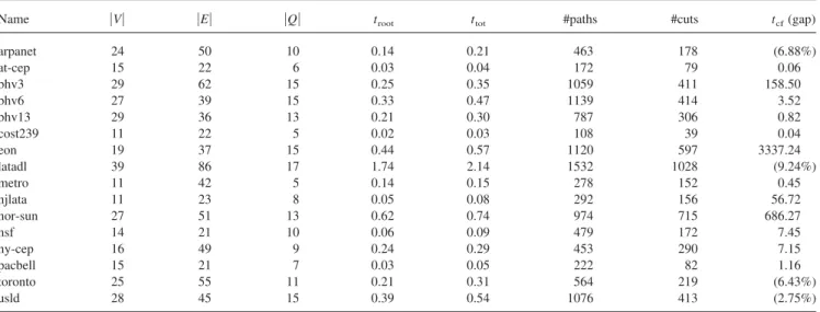
4. COMPUTATIONAL RESULTS
We have tested the compact linear MIP formulations and our BPC algorithm for Sym-G, Asym-G and Rob-G on medium to large-size network topologies. The following instances have been considered:
bhv3/6/13: instances of a multicommodity flow problem
studied in [2];
arpanet, eon, latadl, nsf, pacbell, toronto, usld:
topolo-gies of well-known backbone networks found in the IEEE literature;
res1/5/6/7/8/9, at-cep, ny-cep, nor-sun: instances of
dif-ferent multicommodity flow problems found at http:// www.di.unipi.it/di/groups/optimize/Data/ MMCF.html#Rsrv;
stein1/2/3/4: a set of Steiner tree problem instances with 50
and 75 nodes, available at the Web page http://www. brunel.ac.uk/depts/ma/research/jeb/orlib/ steininfo.html;
n45, n49, n147: general multicommodity flow instances; g200: a network topology with 200 nodes and 914 links
(instance originating from Dan Bienstock and provided by Pasquale Avella, 2004);
t3-X, t4-X: a set of backbone networks with 250 and 304
nodes randomly generated with the gt-itm software (http://www.cc.gatech.edu/projects/gtitm/ gt-itm/).
All instances are available from ftp://ftp.elet.
polimi.it/users/Pietro.Belotti/mcf/vpn in
a pseudo-DIMACS format and in AMPL data format. Because single VPNs are considered, the set Q of termi-nals has been randomly selected as a small subset of V with a density兩Q兩/兩V兩 of approximately 15%. The values of bs, bs⫹, bs⫺, d⬘st, and dˆsthave been generated based on realistic
random traffic matrices.
All tests have been carried out with a Pentium Xeon 2.8 GHz processor, running under Linux with 2 GB of memory available. The BPC algorithm has been implemented in C⫹⫹ using the open-source COIN/Bcp software frame-work (http://www.coin-or.org/documentation.html#BCP) and Cplex 8.1 as LP solver, while Cplex 8.1 MIP solver has been used for our compact formulations. Initially we gen-erate, for each terminal pair (s, t), K shortest paths from s to t through the HREA algorithm described in [13].
The computational results are summarized in five tables that include the following information:
● the instance name and the network parameters (the car-dinalities of V, E, and of the set of terminals Q債 V),
● the time (troot) spent by column generation in the root node, that is, the time required to solve the relaxed prob-lem, starting with K⫽ 5 paths for each terminal pair,
● the time (ttot) spent in total by the BPC algorithm,
● the time (tcf) spent by the Cplex 8.1 MIP solver on the linear flow-based compact formulation,
● #paths and #cuts: the number of paths and cuts generated by the pricing and the cutting-plane iterations.
All times are expressed in seconds.
A time limit of 2 hours has been given both for the BPC algorithm and for tackling the compact flow-based formu-lations with the Cplex 8.1 MIP solver. If the time limit is reached before obtaining an optimal solution, we report in brackets the gap between the best feasible solution and the best lower bound that have been found. A “—” indicates that no feasible solution was found (in the ttot column it
means that the branch-and-bound part was not performed). The label “mem” indicates that the problem could not be solved because of excessive memory requirements, namely more than 2 GB of RAM. In the BPC algorithm, if the time limit is reached while solving the linear relaxation, the gap is given in brackets in the trootcolumn.
According to Table 1, the small-size Sym-G instances (with up to 40 nodes) are solved very rapidly and the performance of Cplex 8.1 on the compact linear MIP for-mulation and of the BPC algorithm are comparable in most cases.
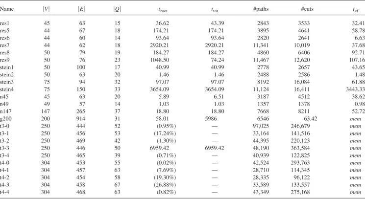
The computational results obtained for larger Sym-G instances are reported in Table 2. Our compact flow-based formulation turns out to be very tight so as to yield the optimal solution within less than a minute even for the large problem “n147.” For larger instances, however, it pays to develop a specialized combined branch-and-price and cut-ting-plane method because the compact linear MIP formu-lation leads to excessive memory requirements. Our BPC algorithm, which performs better on “n147” and on a few smaller instances such as “n45” and “stein2,” allows us to solve “g200” and “t3-3” optimally within the 2-hour time limit and to tackle larger instances. Unlike other experi-ments, for “t3-0” we have set K ⫽ 20 (instead of K ⫽ 5) and let the BPC method run for 252286.68 sec. The gap is in fact reduced to 3.24% after 79293.58 seconds and then progressively to 0.95%. Tuning the value of K and allowing for more than 2 hours of computing time, we can also obtain gaps below a few percentage points for the other large instances. Note that, for all instances that have been solved to optimality, an optimal solution is already found at the root node of the branch-and-price tree. The BPC algorithm stops after the initial column generation phase because the solution found has the same value as the optimal integer solution. In very few cases branch-and-bound steps are performed (and the branch-and-price time taken after the RLP is solved, ttot⫺ troot, is negligible in most cases) and
they do not improve the lower bound. Because the number of paths that are generated during the column generation phase is moderate with respect to the number of terminal
pairs, the approach is viable even for larger instances. The insertion of cutting planes has a dramatic effect in limiting the tailing off of the objective function value when addi-tional paths are added, thus helping to close the gap within a very short computing time. Notice that the number of cuts separated at the root node is the same order of magnitude as the number of paths.
Another interesting result emerged from preliminary ex-periments performed on small, randomly generated Sym-G instances. We have observed that for most instances even the linear relaxation has an integer solution, that is, all flow variables y are either 0 or 1; in the few cases where at least
one y variable is fractional, restoring the integrality con-straints gives an integer solution with the same cost. More-over, for most Sym-G instances the edges {i, j} with pos-itive capacity xij formed a tree; in the remaining cases,
imposing a tree structure on the solution, that is, solving the related Sym-T problem, yielded a solution with the same cost. Thus, our experimental results support the following conjecture:
Sym-G always admits an optimal tree solution.
The same conjecture was also made by Erlebach and Ru¨egg
TABLE 1. Results for small Sym-G instances: BPC algorithm and the compact linear MIP formulation solved with Cplex.
Name 兩V兩 兩E兩 兩Q兩 troot ttot #paths #cuts tcf
arpanet 24 50 10 11.03 11.03 1219 1055 1.97 at-cep 15 22 6 0.02 0.02 211 100 0.03 bhv3 29 62 15 2.65 — 1695 1498 8.34 bhv6 27 39 15 0.14 0.03 1123 648 0.13 bhv13 29 36 13 0.48 0.04 1027 1212 0.86 cost239 11 22 5 0.02 0.02 129 46 0.07 eon 19 37 15 0.49 0.49 1272 714 1.28 latadl 39 86 17 397.27 397.27 3917 4259 219.55 metro 11 42 5 0.01 0.01 126 44 0.26 njlata 11 23 8 0.14 0.14 405 212 0.33 nor-sun 27 51 13 70.53 70.53 2019 1604 64.24 nsf 14 21 10 0.45 0.45 672 422 0.86 ny-cep 16 49 9 0.71 0.71 573 354 0.75 pacbell 15 21 7 0.09 0.09 294 176 0.16 toronto 25 55 11 2.53 2.53 1026 887 6.27 usld 28 45 15 7.55 7.55 1753 1496 4.17
TABLE 2. Results for medium-to-large-size Sym-G instances: BPC algorithm and the compact linear MIP formulation solved with Cplex.
Name 兩V兩 兩E兩 兩Q兩 troot ttot #paths #cuts tcf
res1 45 63 15 36.62 43.39 2843 3533 32.41 res5 44 67 18 174.21 174.21 3895 4641 58.78 res6 44 60 14 93.64 93.64 2820 2641 6.63 res7 44 62 18 2920.21 2920.21 11,341 10,019 37.68 res8 50 79 19 184.27 184.27 4860 6406 92.71 res9 50 76 23 1048.50 74.24 11,467 12,620 107.16 stein1 50 100 17 40.99 40.99 2778 2657 43.65 stein2 50 63 20 1.46 1.46 2488 2586 1.48 stein3 75 94 32 97.07 97.07 8192 16,084 61.88 stein4 75 150 33 3654.09 3654.09 11,124 16,411 3443.33 n45 45 63 20 5.89 6.51 3187 4512 38.62 n49 49 57 14 1.03 1.03 1357 1378 0.98 n147 147 265 37 18.80 18.80 7668 8211 52.72 g200 200 914 31 58.01 5986 6546 63.42 mem t3-0 250 444 52 (0.95%) — 97,025 246,679 mem t3-1 250 456 53 (17.24%) — 33,164 141,516 mem t3-2 250 469 42 (1.30%) — 44,395 220,123 mem t3-3 250 446 50 6959.42 6959.42 48,190 363,584 mem t3-4 250 465 39 (0.71%) — 40,939 122,825 mem t4-0 304 453 55 (0.02%) — 42,524 293,763 mem t4-1 304 457 63 (7.69%) — 28,710 114,345 mem t4-2 304 454 58 (19.30%) — 28,335 96,122 mem t4-3 304 458 67 (26.88%) — 33,589 133,557 mem t4-4 304 468 63 (0.82%) — 43,349 275,168 mem
[8] and it has been proved by Hurkens et al. [12] for networks consisting of a single cycle. Note that the situation for Asym-G differs slightly: most instances have an integer optimum with the same cost as the linear relaxation optimal solution, but we have found some instances with an integer optimum with larger cost.
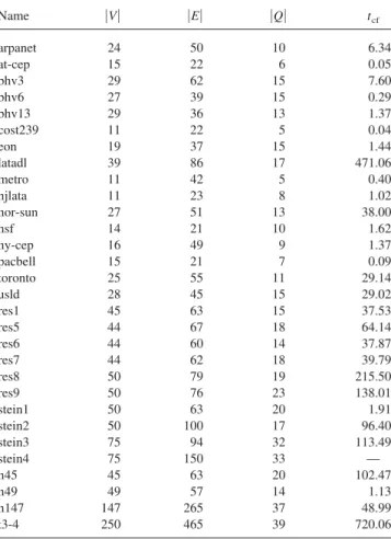
Computational results for Asym-G are reported in Table 3. The compact flow-based formulation is remarkably tight and effective also in this case. All mid-size instances can be solved to optimality in a few minutes with the Cplex 8.1 MIP solver, except for “stein4,” for which no integer solu-tion could be found within the time limit. Among the large networks, only “t3-4” could be solved to optimality, whereas the remaining “tX-X” and “g200” could not be solved due to excessive memory requirements. In general, asymmetric instances appear to be more challenging than symmetric ones for the BPC approach. Because for 9 out of the 40 instances considered the gap remains large after reaching the time limit, we do not report BPC computing times.
It has still to be determined whether the substantial difference observed for several instances is mainly due to the remarkable quality of the compact linear MIP formula-tion or to a relevant margin for improving the BPC algo-rithm, by including for instance efficient memory manage-ment procedures that purge unused paths/cuts and
variables. However, we should point out that passing from the symmetric to the asymmetric Hose models renders the problem significantly harder. This is indeed the case for
Sym-T and Asym-T. Although Sym-T can be solved by
repeated application of shortest path algorithms, Asym-T is strongly NP-hard. Concerning the behavior of the branch-and-price algorithm, we should notice that the number of variables in the Asym-G MIP formulation (18)–(23) is twice the number of variables in the Sym-G formulation. We believe that this increase in the number of variables nega-tively affects the pricing and separation phases of the BPC algorithm. We have observed this in a few numerical ex-amples that we did not report in the tables because the running times were worse than with the compact formula-tion. Let us consider the three examples res1, stein1, and n147. For the Sym-G case from Table 2, we see that res1 was solved to optimality by generating 2843 paths and 3533 cuts. The same statistics when we pass to Asym-G uncertainty problems are 4972 and 5952, respectively. For stein1, in the Sym-G case the number of paths and cuts were 2778 and 2657, respectively. Passing to Asym-G, these numbers become 5628 and 17225, respectively. Finally, in the n147 case, we have 7668 paths and 8211 cuts in the
Sym-G case and 9823 paths and 35629 cuts for Asym-G.
This seems to be a pattern for almost all test problems. The results obtained for Rob-G are summarized in Tables 4 and 5. Here,⌫ is taken equal to 15% of the total number of terminal pairs, but other intermediate values yield similar results. Although the robust VPN provisioning problem leads to less conservative VPNs by exploiting the available traffic statistics, Tables 4 and 5 indicate that the correspond-ing compact linear MIP formulation is much harder to tackle with Cplex 8.1 than those for Asym-G and Sym-G. However, the BPC algorithm is remarkably effective in solving Rob-G instances, and it compares very favorably with Cplex 8.1 even for small-size instances. As happens with Sym-G, the compact flow-based formulation for Rob-G requires more memory than the BPC algorithm in which paths and cuts are dynamically generated starting from small initial sets. For all instances larger than “n147,” the compact formulations do not fit within 2 GB of RAM, whereas the path-and-cut formulations, which have a poten-tially exponential size, lead to optimal solutions in less than 2 hours. Note that only a limited number of paths and cuts are generated.
The improved performance of the BPC for this uncer-tainty model cannot be related to a lower dimensional demand polyhedron as might be between Asym-G and
Sym-G (see discussion above), because there is a large
increase in the number of variables in Rob-G with respect to
Asym-G. Therefore, we cannot say that it is just the number
of variables that affects the performance of the BPC algo-rithm. Our partial explanation for this is the favorable struc-ture of the polyhedron that results from the Bertsimas and Sim constraints. More specifically, although 2兩S兩 ⫹ 1 ⫽ 兩Q兩(兩Q兩 ⫺ 1) ⫹ 1 constraints describe the latter and only 2兩Q兩 are needed for Asym-G (Q being the set of terminal
TABLE 3. Results for Asym-G instances: Compact linear MIP
formulation solved with Cplex.
Name 兩V兩 兩E兩 兩Q兩 tcf arpanet 24 50 10 6.34 at-cep 15 22 6 0.05 bhv3 29 62 15 7.60 bhv6 27 39 15 0.29 bhv13 29 36 13 1.37 cost239 11 22 5 0.04 eon 19 37 15 1.44 latadl 39 86 17 471.06 metro 11 42 5 0.40 njlata 11 23 8 1.02 nor-sun 27 51 13 38.00 nsf 14 21 10 1.62 ny-cep 16 49 9 1.37 pacbell 15 21 7 0.09 toronto 25 55 11 29.14 usld 28 45 15 29.02 res1 45 63 15 37.53 res5 44 67 18 64.14 res6 44 60 14 37.87 res7 44 62 18 39.79 res8 50 79 19 215.50 res9 50 76 23 138.01 stein1 50 63 20 1.91 stein2 50 100 17 96.40 stein3 75 94 32 113.49 stein4 75 150 33 — n45 45 63 20 102.47 n49 49 57 14 1.13 n147 147 265 37 48.99 t3-4 250 465 39 720.06