• Sonuç bulunamadı

Revisiting the Finance-Growth Nexus in Turkey: Bayer-Hanck Combined Cointegration Approach over the 1970-2016 Period

N/A
N/A
Protected

Academic year: 2021

Share "Revisiting the Finance-Growth Nexus in Turkey: Bayer-Hanck Combined Cointegration Approach over the 1970-2016 Period"

Copied!
28
0
0

Yükleniyor.... (view fulltext now)

Tam metin

(1)

Date Accepted: 07.02.2020 2020, Vol. 28(44), 41-68

Revisiting the Finance-Growth Nexus in Turkey: Bayer-Hanck

Combined Cointegration Approach over the 1970-2016 Period

Onur ÖZDEMİR (https://orcid.org/0000-0002-3804-0062), Department of International Trade, İstanbul Gelişim University, Turkey; e-mail: onozdemir@gelisim.edu.tr

Türkiye’de Finans-Büyüme Bağıntısının Yeniden Değerlendirilmesi:

1970-2016 Dönemi için Bayer-Hanck Bileşik Eşbütünleşme Yaklaşımı

Abstract

This study revisits the finance-growth nexus in Turkey for the period between 1970 and 2016. The econometric analysis is based on the Bayer-Hanck combined cointegration test to examine whether the cointegration exists or not between the related variables. The results of the Bayer-Hanck combined cointegration test show that there is no cointegration between financial development and economic growth even in the control of other variables such as economic globalization and technological progress. The estimation results also reveal that the long-run linkage is not prevailing between the variables. In other words, it can be argued that financial development does not contribute to the economic growth process by way of higher levels of economic globalization and technological progress in the long-run.

Keywords : Financial Development, Economic Growth, Economic Globalization, Technological Progress, Bayer-Hanck Combined Cointegration Test. JEL Classification Codes : F3, F6, O3.

Öz

Bu çalışma, Türkiye’deki finans-büyüme bağıntısını tekrar ele almaktadır. Örneklem 1970 ve 2016 arası dönemi kapsamaktadır. Ekonometrik analiz, değişkenler arasında eşbütünleşmenin var olup olmadığını incelemek için Bayer-Hanck bütünleşik eşbütünleşme testine dayanmaktadır. Bayer-Hanck bileşik eşbütünleşme testi sonuçları, ekonomik küreselleşme ve teknolojik ilerleme gibi kontrol değişkenlerinin varlığında dahi finansal gelişme ve ekonomik büyüme arasında eşbütünleşme olmadığını göstermektedir. Tahmin sonuçları ayrıca değişkenler arasında uzun vadeli bir ilişkinin olmadığını ortaya çıkarmaktadır. Diğer bir deyişle, finansal gelişmenin, uzun vadede, yüksek ekonomik küreselleşme ve teknolojik ilerleme yoluyla ekonomik büyüme sürecine katkıda bulunmadığı ileri sürülebilir.

Anahtar Sözcükler : Finansal Gelişme, Ekonomik Büyüme, Ekonomik Küreselleşme, Teknolojik İlerleme, Bayer-Hanck Bileşik Eşbütünleşme Testi.

(2)

1. Introduction

Numerous studies have been substantially pointed out the positive relationship between financial development and economic growth. In other words, they have been argued that a higher level of financial development plays a critical role in an increase in the level of economic development. According to the traditional arguments which favor this positive link between financial development and economic growth, the more developed financial system ensures a long-run sustainable growth by facilitating the intermediation process between lenders and borrowers. In particular, this is highly prevailing in developing countries since they have a great deal of potential to provide higher returns for foreign capital. The major way to do this is to increase interest spread in those countries in contrast to the developed countries, which extract an extra surplus of capital located abroad. Therefore, if this amount of surplus are used in profitable investment opportunities, the levels of economic development among these country groups will be converged to each other. This is only possible for the countries where the levels of financial development are significantly high. Hence, the positive link between financial development and economic growth needs to be dealt with significant attention in the literature, especially for the case of developing countries.

Turkey is one of the leading countries which has different types of financial instruments using in financial relations; and thus, attract foreign investors to invest in the financial sector. However, the roots of the financial sector development in Turkey are not very old but mainly depend on a very near future. Figure 1 shows the historical background of the financial development process for the period between 1980 and 2016. The overall index for financial development shows the weighted average of two specific indices which are financial market development and financial institution development. Though these two sub-indices are different from each other, they were being in an increasing trend since the 1980s. Therefore, it needs some attention to understand the reasons behind this ongoing trend of financial development. For instance, whereas the pre-1994 period is somehow steady, each index exacerbated after 1994 and peaked in 2014. As one can see that the crisis periods indicate that the financial sector negatively affected by economic issues. One of the major downturns in financial development was placed in 1994 and 2001, which of these two basic periods correspond to severe economic crises in Turkey. However, on average, financial development has reached historical records in the Turkish economy.

(3)

Figure: 1

Financial Development in Turkey

Source: Svirydzenka (2016).

These financial dynamics of the Turkish economy lead us to investigate the nature of the causal relationship between financial deepening and economic development. In addition to these two specific variables, we consider that financial components are highly correlated with the economic globalization indicators such as openness indices for trade and finance. Therefore, we add the economic globalization indicator into the analysis as another critical source for the economic conditions.

The growing body of empirical study in traditional wisdom produces commonly similar outcomes which of those depend on close methodological considerations and use similar data sets. In general, economic results can be categorized as follows (Levine, 2004). First, the countries tend to have higher economic growth rates if they have developed financial sector. In that vein, better-developed financial sector includes two major sub-components which are the level of banking development and the liquidity of stock markets. Each of these components exerts a positive effect of economic growth. Second, the external financing constraints can be eased by providing better-functioning of the financial sector. Third, better access to capital, especially to foreign capital, should be provided by a higher level of financial development and a higher rate of economic growth. However, none of these components specify the importance of economic globalization. It should be examined that the causal linkage between financial development and economic globalization can be effective to produce a higher level of economic growth. However, depending on other economic conditions of the country, the reverse can also be true for the same case.

To best of our knowledge, there is no any kind of analysis related to this issue in case of Turkey. While some of the studies focus on the causal linkages between financial development and economic growth, the others examine more specific indicators for finance

0,00 0,10 0,20 0,30 0,40 0,50 0,60 0,70

(4)

related to economic development. Hence, many of them ignore the role of economic globalization which has been very crucial in determining the causal relationship between financial development and economic growth. The aim of this paper, therefore, is to reveal direct linkages between financial deepening, economic globalization and economic development for Turkey and to test the significance of traditional knowledge about the positive causal relationship between finance and economic development by employing yearly data for the period between 1970 and 2016.

In particular, this paper provides some answers for the question of whether financial deepening and economic globalization lead economic development or of whether economic development produces a higher degree of economic globalization and financial deepening in Turkey, which of those variables can be interrelated with each other. In this sense, instead of linear causality analysis, the empirical content implies the nonlinear causality test to examine whether the causal relationship among the variables of interest is affected from the structural breaks and asymmetries in the series that we employ in the analysis. In brief, the results of combined cointegration approach imply that there is no cointegration between financial development and economic growth.

This study is composed of four parts. The second part explains the theoretical specifications for financial development and economic growth, which are remarkably based on traditional knowledge. This part also specifies some major indicators that are used in the empirical analyses of different studies. The third part focuses on data description, methodological framework, and the empirical results. In addition, it provides some stylized facts about the financial sector development in Turkey together with the globalization movements and economic development process.

2. Financial Development and Economic Growth: Theoretical and Empirical Discussions

2.1. Theoretical Considerations

The theoretical examinations on finance-growth nexus can be traced back to Bagehot [1873] (2015), Schumpeter [1934] (1981), Gurley and Shaw (1955), Patrick (1966), Goldsmith (1969) and Hicks (1969). In that sense, the studies on the empirical side of this nexus become favorable after the 1970s. Bagehot [1873] (2015), one of the earliest pioneers, who implicitly investigated the relationship between finance and growth. The major aim of Bagehot [1873] (2015) is to show the impact channels of financial market development on capital flows and to examine the transformation mechanism of financial intermediaries for savings which is converted into long-term investments. According to Bagehot [1873] (2015), both of these factors are highly influential in economic growth. Similar to Bagehot [1873] (2015), Schumpeter [1934] (1981) essentially pointed out the importance of finance for economic growth. Schumpeter [1934] (1981) argued that the banking sector should be strong for a higher rate of economic growth which stimulates technological progress; and thus, encourage the lowest cost production method.

(5)

Along with this knowledge, Gurley and Shaw (1955), Goldsmith (1969) and Hicks (1969) indicated that the under-developed financial system is harmful to long-run economic growth. Therefore, the higher rates of economic growth can only be obtained by a higher level of financial development. Following the same conceptualization, Patrick (1966) developed a new way to understand the demand- and supply-side conditions, namely demand-following and supply-leading, in case of the distinction between the real sector and the financial sector1. While the former indicates that the financial services are highly

dependent on the demand conditions in the real sector2, the latter states that the financial

sector has a leading role in promoting long-run economic growth3. According to Patrick

(1966), the direction of causality between finance and growth is thus highly controversial in the literature4.

The data scarcity was the common problem for an investigation of the effectiveness of both supply-leading and demand-following hypotheses, especially in terms of developing economies. The period after the 2000s has witnessed that time series analyses based on the causality approach have become more popular than cross-section analyses since the results might be different but also might have adverse theoretical considerations. The first group of analyses, which are based on time-series methods, have substantially employed two major variables consisting of financial development and economic growth to test the causality linkages between these two variables. The second group includes analyses that used cross-section methods in which the economic growth indicators were regressed on measures of financial development in control of set of variables. Therefore, the econometric models are various in the literature including pooled Ordinary Least Squares (OLS), fixed-effects, random-effects and multivariate causality. However, the empirical results are mixed and controversial, especially for the case of regressions applied for developing countries. One of the major reasons might depend on the selection of proxy variables for financial development or alternatively, might depend on the failure of the adoption of the empirical procedure that was used in the analyses.

The theoretical structures of both demand- and supply-side conditions are to a large extent produced by two fundamental knowledge which consists of the Structuralist School

1 Note that the two-way causality relationship between finance and growth primarily postulated by Lewis (1955) and then supported by Patrick (1966).

2 For instance, Robinson (1952: 86) argues that “by and large, it seems to be the case that where enterprise leads, finance follows”.

3 Habibullah and Eng (2006) point out the importance of the latter view by turning the attention to the finance-led growth discussions which have been very popular in developing country groups as an engine for a higher level of economic development.

4 Whereas one-way causality direction is very widespread among individual country case studies, some of the panel studies also show that the bi-directional view is possible under some conditions for finance-growth nexus. Related to this framework, King and Levine (1993a: 730) pointed out that “the link between growth and financial development is not just a contemporaneous association. Finance does not only follow growth; finance seems importantly to lead economic growth”.

(6)

and the Neoclassical School. First, according to the Structuralist School, the financial sector as a whole should be expanded by way of an increase in financial instruments, financial resources or financial tools used in finance-based transactions5. Second, the Neoclassical

School essentially encourages a higher degree of financial openness in the financial sector, by which it argues that any control or restriction related to the financial relations should be eliminated by the monetary authorities6.

In addition to this distinction, the finance-led growth hypotheses are also interpreted within the context of the relative significance of the differences between bank-based and market-based financial system. According to Gerschenkron (1962), banks are the major unit for the financial intermediation process. In that vein, banks are more effective for the allocation of the resources in case of funding and intermediating processes compared to the stock markets. Hence, the banking sector should be well-developed and well-functioning as well. However, the advocates of market-based financial system follow a different way to interpret the effects of the financial development on economic growth. According to them, financial markets should be liquid and strong to obtain a long-run economic growth, which basically provide the necessary amount of capital to the firms for their further investments that subject to technological progress (Allen & Gale, 1999).

The debate on the finance-led growth hypothesis has been further examined by the emergence of endogenous growth theory produced by Romer (1986) in the mid-1980s. According to this theory, financial intermediaries such as banks and other financial institutions provide an improvement in the efficiency of investment and thus a higher level of financial development can be assumed as one of the leading components for a higher rate of return (Renelt, 1991). The major findings within the case of endogenous growth theory can be classified as follows. First, the economic growth might be affected positively by an increase in financial development if it relies upon more productive investments through advanced coordination of liquidity risks (Bencivenga & Smith, 1991). Second, financial development might accelerate the process of economic growth if the information is collected on the efficiency of investment projects and/or investor’s abilities (Greenwood & Jovanovic, 1990). Third, if there is an efficient diversification of investors’ portfolios, financial development might lead to a higher rate of economic growth (Levine, 1991; Saint-Paul, 1992). All in all, both of these various arguments on endogenous growth theory implicitly state that producing a higher level of financial development leads to the reduction of information and transaction costs which result in the efficient allocation of resources.

Furthermore, Kar et al. (2014) classify the determinants of the differences in the level of financial development after 2000s as follows: (i) Legal origin (Demetriades, 2008); (ii)

5 For instance, the arguments of Goldsmith (1969) and Patrick (1966) can be categorized in the Structuralist School.

6 For more theoretical detail about the relationship between financial liberalization and economic development, please see McKinnon (1973), Shaw (1973) and Fry (1978).

(7)

public bank ownership (La Porta et al., 2002; Andrianova et al., 2008); (iii) initial conditions and institutional structure (Acemoglu et al., 2001, 2004); (iv) trade liberalization (Huchet-Bourdon et al., 2018); (v) financial openness (Chinn & Ito, 2006; Klein & Olivei, 2008); (vi) prudential supervision and effective regulation (Brownbridge et al., 2005); (vii) required reserves (Arestis et al., 2002); and (viii) macroeconomic policies (Bittencourt, 2011).

Although the traditional wisdom supports that there is a positive and significant relationship between financial development and economic growth even if the causality among these variables is uni- or bi-directional, there are also some counter-views on this topic which of those focus on destabilizing effect of an increasing scale of stock markets on aggregate economy in case of inability of risk diversification in the financial sector. For instance, Minsky (1975) argues that the unstable basis of the financial system may lead to the emergence of financial crises. In addition, Keynes (1964) indicates the importance of the speculative motive in financial relations which may have a negative impact on the stability of economic conditions.

2.2. Empirical Discussions

The empirical studies in favor of the traditional wisdom which relate the uni-directional causality from financial development to economic growth argue that this linkage can be through three main channels (Aziz & Duenwald, 2002). First, financial development can increase the marginal efficiency of capital by way of collecting information for alternative investments and risk diversification. Second, financial development can raise the marginal propensity to save; and thus, it can enhance the efficiency of intermediation process of financial relations. Third, financial development can raise the level of savings made by households and firms.

An extensive amount of empirical studies has found that the finance-growth nexus is significant for the case of different types of regression methods, aimed at examining the theoretical considerations of the directions of the causality between financial development and economic growth. In brief, the common results of orthodox studies provide strong evidence that there is a uni-directional correlation among these two variables, from finance to growth. This is also consistent with the earlier arguments which were essentially based on the importance of the linkage between finance and growth. For instance, whereas the data availability restricted the higher evidence for the causality linkage among the finance-growth nexus, the earlier proponents of this uni-directional causality proposed by Goldsmith (1969), McKinnon (1973), Shaw (1973) and Fry (1978) found that an implementation of a higher degree of financial liberalization in the economy would stimulate the growth rates and thereby increase the amount of real output. Therefore, many of the recent studies have pointed out the positive impact of a higher level of financial development on economic growth.

On the one hand, cross-country and panel data analyses provide a positive relationship for finance-growth nexus in control of several indicators of growth and of statistical and econometric problems such as simultaneity bias, reverse causality, omitted

(8)

variable bias and unobserved country-specific effects. On the other hand, time-series studies provide another part of the empirical outcomes on finance-growth nexus but they are controversial and have some mixed results about the direction of causality.

First, many of these studies7 suggest that finance is the engine of economic growth.

However, the reasons behind this uni-directional causality analysis are several. According to King and Levine (1993a), a developed financial system leads to a higher level of productivity and support potential entrepreneurship. Hence, providing an improvement in the productivity stimulates innovation-enhancing activities and thereby the sustainable economic growth. Similarly, Bencivenga and Smith (1993) argue that the financial intermediaries8 can have potential effects to reduce the credit rationing and monitoring costs

in a well-functioning financial system; and thus, they lead to a higher level of production in real output by way of an efficient allocation of resources. In addition, growth-enhancing financial regulations implementing in the financial system can increase the specialization and can reduce the transportation costs which then boost the productivity level in control of a simultaneous increase in the exchange of goods and services (Greenwood & Jovanovic, 1990). Newly emerged financial instruments in the financial system as a whole facilitate the exchange of goods and services by fulfilling the needs of rapidly changing developing economies (Greenwood & Smith, 1997; Levine; 1997).

Second, another view on this uni-directional causality linkage follows the rule that the direction of causation runs from economic growth to financial activity. Robinson (1952) argues that financial activity is a part of economic development; and thus, the growing economy needs for a higher demand for financial services which results in the development of financial sector itself due to this strong correlation among finance and economic development. The arguments suggested by Robinson (1952) are also the basis of the demand-following hypotheses. In addition to Robinson (1952), Kuznets (1955) and Friedman and Schwartz (1963) follow the idea that economic growth enhances financial development. Patrick (1966) points out that the increasing demand in the real sector specifically needs more developed financial institutions and services. In that vein, according to Stern (1989) and Romer (1990), financial sector development is facilitated by real sector development9.

7 For more information on earlier studies, please see Goldsmith (1969), McKinnon (1973), Shaw (1973), Kapur (1976), Galbis (1977), Fry (1978, 1995) and Mathieson (1980).

8 Some of the factors that positively affect the economic growth can be classified as follows: (i) the contribution to the efficient allocation and supervision of savings; (ii) ensuring the transfer of savings to the investments; (iii) the orientation of available funds to the innovative projects by reducing the asymmetric information; (iv) tracing the performance of managers; and (v) providing of the realization of financial transactions (Besci & Wang, 1997; Boyd & Prescott, 1986; Capasso, 2004).

(9)

Third, the final part of the studies suggests that there is a bi-directional causality and simultaneous relationship between finance and growth10. In essence, Greenwood and

Jovanovic (1990) state that financial intermediaries such as banks and other financial institutions support profitable projects and economic growth by way of increasing the rate of return on capital, and that growth-enhancing process leads to an expansion of financial instruments and a raise of the impact of financial services on economic indicators. Therefore, the causality runs in both directions simultaneously. In the same vein, some other studies suggesting that there is a bi-directional causality between finance and growth imply that the economic growth increases the level of quality of financial instruments and the number of financial activities stimulated by the banking sector (Ireland, 1994; Demetriades & Luintel, 1996; Luintel & Khan, 1999).

Apart from the major hypotheses called “supply-leading” and “demand-following”, there are also two other empirical considerations in the literature. On the one hand, there is no causality linkage between financial development and economic growth at all11. According

to this kind of argument, the potential correlation among these two major variables is spurious (Lucas, 1988). In other words, the financial sector and thereby the economy as a whole can grow in the future period, depending on different types of indicators and different socio-economic and political conditions, which means that they all follow their own way (Graff, 2001). In addition, there may be non-uniformity of the finance-growth nexus since the relationship between financial development and economic growth is provided in the short-run but the determinants of the long-run cause a reversed U-shaped linkage among two indicators12. On the other hand, financial activity can have a negative impact on a higher

level of economic development. The proponents of this view argue that the direction of causality runs from finance to growth but in a negative manner. According to this view, finance has a destabilizing effect on sustainable economic growth, which can be resulted in the economic crises by affecting the financial sector as a whole. Specifically, the financial sector has inherently unstable and thus can negatively affect the major channels of economic growth and development. Therefore, implementing a higher level of financial development can repress the long-run economic growth by reducing the potential credit sources available to the domestic firms (Minsky, 1975; van Wijnbergen, 1983; Buffie, 1984; Xu, 2000).

According to McKinnon (1973) and Shaw (1973), the channels that implement the liberalization of financial sector also need a higher level of financial development, which

10 For instance, some of the major studies on the basis of a bi-directional causality between finance and growth can be ranged as follows: Bencivenga and Smith (1991), Roubini and Sala-i Martin (1992), Pagano (1993), King and Levine (1993a), Barthelemy and Varoudakis (1996), Demetriades and Hussein (1996), Greenwood and Smith (1997), Levine (1997), Blackburn and Hung (1998), Calderón and Liu (2002), and Yaprakli (2007). 11 For instance, Lucas (1988) notes that some economists “badly over-stress” the impact of financial components

on economic growth and development.

12 For more empirical information on these controversial results, please see Cecchetti and Kharroubi (2012), Arcand et al. (2015), Samargandi et al. (2015), Deidda and Fattouh (2002) and Rioja and Valev (2004).

(10)

then leads to an increase in the economic growth. In other words, one of the major conditions for the liberalization of the financial sector as a whole highlight the importance of lifting any sort of restrictions on the free movement of capital all over the world. The liberalization of financial sector consists of two important phases. The first stage is the elimination of some regulatory practices that prevent the free entry of new institutions into the financial system. Following the first stage, the second stage is the development of financial institutions and financial markets. These stages are the basis of the initial conditions for an implementation of more liberalized financial system. One of the main conditions in this process is to increase real interest rates. This follows the increases in the total savings and the funds to be used in profitable projects. Therefore, the synchronization between higher level of savings and higher level of investment can be provided. The empirical investigations show that there is a positive correlation between the positive real interest rates and a higher rate of economic growth in the context of different methods. In other words, the proponents in favor of a more liberalized financial sector imply that the positive real interest rates positively affect the long-run economic growth (Galindo et al., 2007; McKinnon, 1991, Neusser & Kugler, 1998; Kang & Sawada, 2000; King & Levine, 1993a, 1993b; World Bank, 1989).

In addition, according to the McKinnon-Shaw hypothesis, the implementation of ceilings on deposits and loan rates can negatively affect economic growth and development. The ceilings on nominal interest rates decrease the degree of financial depth and thereby negatively affect the growth rates. An interest rate ceiling basically causes four different consequences which are affected each other (Andersen & Tarp, 2003): (i) the formation of negative interest rates; (ii) the reduction of the amount of loanable funds; and (iii) the inefficient allocation of resources; and (iv) the reduction in the marginal efficiency of capital. Both of these factors have negative effect on long-run economic growth. Moreover, McKinnon (1973) and Shaw (1973) jointly assert that the liberalized financial system should incorporate more open trade regimes and unrestricted capital flows13.

The finance-growth nexus is also investigated in terms of the difference between bank-based and market-based analyses. Primarily, financial systems are divided into two parts as bank-based and market-based in case of their structural characteristics and significance in the market (Targan, 1996). On the one hand, the proponents of the bank-based financial system argue that the unique success achieved in the industrialization process and in the technological progress basically depend on the consequences of providing the further needs for funds of banks. Therefore, the historical movements in favor of the implementation of more bank-based rules in the financial system substantially lead to a higher level of economic growth in the long-run14. In bank-based systems, banks have some

major roles in critical economic conditions such as the mobilization of savings, the allocation of capital, the control of investment decision of corporate managers, and the providing of

13 For more information, please see Calvo and Coricelli (1992) and Chandrasekhar (2004). 14 For more information, please see Bhide (1993) and Levine (2004).

(11)

risk management vehicles. On the other hand, the proponents of market-based financial system state that a simpler, safe, strong and more stable stock markets become more active and efficient than banks. For instance, in the market-based systems, banks and the markets for securities markets have the same weights in transferring savings to firms, exerting corporate control, and facilitating risk management15. However, some others which are used

the theoretical considerations of both systems argue that these factors complement each other. Therefore, the important point here is to investigate whether the financial markets are efficient or not. A simpler, safer, strong, more diverse and more stable financial system can have a higher potential to affect economic growth (La Porta et al., 1998; Levine, 2004).

The empirical investigations on the relationship between financial development and economic growth have been popular after the mid-1980s along with the emergence of the endogenous growth theories. The major difference among these models depends on the fact that the saving behaviors play an active role in the determination of equilibrium income levels and growth rates16. In addition, these new types of growth models have solved the

insufficiency for an explanation of the divergence among countries in terms of their levels of financial development. In that vein, while the main factors behind the impetus of economic growth rates were ignored in the neoclassical growth model (Solow, 1956), these new theories have specifically pointed out the factors which were engines of the long-run growth (Romer, 1986, 1990; Lucas, 1988). The latter models have been grounded on the fact that the technological progress is endogenous and thus need an economics of scale in the production. For instance, some of the major factors affecting the economies of scale can be ranged as follows17: (i) the R&D and innovation (Romer, 1986, 1990); (ii) the government

expenditures (Barro, 1990); (iii) the cumulative capital (Rebelo, 1991); (iv) the financial markets (Pagano, 1993); and (v) the human capital (Lucas, 1988). However, similar to the earlier studies about the direction of causality between finance and growth, the empirical findings in endogenous growth models provide controversial results. For instance, Murinde and Eng (1994) and Luintel and Khan (1999) point out the current studies which are based on the bi-directional relationship between financial development and economic growth. Therefore, even for the endogenous growth theories, the demand-following and supply-leading hypotheses are still apparent and relevant for various amount of empirical studies18.

Numerous empirical studies have argued that countries with an advanced level of financial systems tend to increase their economic growth rates, especially those have well-functioning banking sector and liquid stock markets (Ozturk, 2008: 87). Therefore, there is a growing body of studies which provide some critical arguments that the levels of banking

15 Demirgüç-Kunt and Levine (2001) give many crucial details on the difference between bank-based and market-based financial systems within the case of cross-country roughly includes 150 countries and they use newly collected data on financial indicators.

16 Please see Greenwood and Jovanovic (1990) and Bencivenga and Smith (1991). 17 For an extensive research on this classification, please see Ağır et al. (2009).

(12)

sector development and stock market liquidity exert a positive effect on economic growth, in control of different statistical methods and data sets. For instance, Levine and Zervos (1998), Arestis et al. (2001), Beck and Levine (2004), and Wu et al. (2010) found a positive and statistically significant relationship between financial development, including both banking sector and stock markets, and economic growth. In addition, Seven and Yetkiner (2016) found that the banking sector development has a positive impact on economic growth in low- and middle-income economies. However, it negatively affects economic growth in high-income economies. Puryan (2017) also examined the same hypothesis for MENA countries over the 1988-2012 period and argued that there is a bi-directional causality between stock market development and economic growth and the long-term effect of stock market development on economic growth is positive and significant. Finally, Murari (2017) investigated the finance-growth nexus within the framework of stock markets and banking sector for South Asian countries over the 1980-2003 period. The empirical results showed that financial deepening measured by different variables did not adequately support the economic growth since the financial relations and activities were at very low levels in South Asian countries and there was lack of audit and credit allocation problems. However, the stock market development measured by stock market capitalization ratio and liquidity exerts a positive effect on economic growth.

All in all, the theoretical and empirical considerations on finance-growth nexus can be classified into six different approaches. The first classification is based on the arguments that economic growth follows financial development, which is also called as the supply-leading hypothesis. According to this hypothesis, there is a positive but also a significant linkage between financial intermediation and economic growth. In that vein, the direction of causality is from intermediation process to growth. The pioneers of this approach basically argue that a higher level of economic growth can be provided by the leading process of higher saving rates or by a further increase in capital accumulation. The second classification is grounded on the demand-following hypothesis. This approach implies that a higher level of financial development is stimulated by the demand of the real sector. In other words, the process of economic growth leads to better-developed financial activities. The latter two classifications are on the basis of the uni-directional and bi-directional forms of causality. However, it should be noted that these forms of the direction of causality are somehow controversial due to the fact that the differences of the empirical methods and more specifically, the economic condition of countries can alter the direction of causality and the way that finance and growth follow. On the other hand, the fifth classification shows that there is no causality between finance and growth. Finally, some other studies find that financial development is harmful to the long-run economic growth and development because of several reasons such as the initial conditions of finance and the economic structure.

3. Data, Methodology and Empirical Results 3.1. Data

The data used in the empirical analysis is obtained from Financial Structure Database (Beck et al. 2000, 2009; Ćihák et al. 2012), KOF Globalization Index (Gygli et al., 2019)

(13)

and World Development Indicators elaborated by the World Bank for the variables of financial deepening, economic globalization and economic growth, respectively. The study is also used yearly data for Turkey during the period 1970-2016. Table 1 shows the details on the list of variables.

Table: 1

Variables, Definitions and Sources

Variable Definition Measurement Source

Log(Y) GDP

(constant 2010 US$) Logarithm of constant GDP 2010 US$

World Bank, World Development Indicators FD Financial System

Deposits to GDP (%)

Demand, time and saving deposits in deposit money banks and other financial institutions as a share of GDP

Financial Structure Database

EC Economic Globalization Index

Economic globalization characterizes long-distance flows of goods, capital, and services as well as information and perceptions that accompany market exchanges.

KOF Globalization Index

TFP TFP at constant national

prices (2011=1) The adjusted rate of total factor productivity at national prices, 2011=1 Penn World Tables 9.0

Table: 2 Descriptive Statistics LogYt FDt ECt TFPt Mean 11.6004 26.4956 43.9967 0.9527 Median 11.5983 23.2415 47.6174 0.9495 Maximum 12.0502 46.3349 56.4749 1.0539 Minimum 11.1679 10.9176 28.0030 0.8766 Std. Dev. 0.2500 10.3045 10.0958 0.0441 Variance 0.0625 106.1834 101.926 0.0019 Skewness 0.0757 0.6989 -0.4788 0.2856 Kurtosis 1.9314 2.3055 1.6765 2.4994 Jarque-Bera 2.2326 4.6695 5.1146 1.1054 Figure: 2

Financial System Deposits to GDP Trend in Turkey

Source: Financial Structure Database.

Table 2 provides descriptive statistics for the variables using in the model over the period 1970-2016. Figure 2 shows the trend in financial development data (so-called as financial system deposits to GDP, %). In addition, Figure 3 shows the historical movement of the economic globalization index of Turkey over time. In particular, it can be argued that

0 5 10 15 20 25 30 35 40 45 50

(14)

the increasing trend is very similar to the financial development. While the index is sluggish for the period between 1970 and 1980, it has skyrocketed after the 1980s. However, it should be noted that this increasing trend is not specific to Turkish economy but can also be seen in other countries from both developed and developing country groups. These figures show that all indicators have increased over the sample period. In particular, financial development has been skyrocketed after the 1980s. This is also prevailing for the economic globalization index covering both trade and financial openness measures.

Figure 3:

Economic Globalization Trend in Turkey

Source: KOF Globalization Database.

3.2. Methodology

It is possible that different types of sub-components can either positively or negatively affect the conditions of the economic systems. Therefore, they may lead to contradictory empirical results in determining the causal relationship between the sample indicators. However, even if there are different statistical methods to test the direction of causality among variables, few of them point out the importance of testing endogenous breaks in data over time. In other words, the variables may subject to structural breaks which provide biased estimations. In that sense, instead of using the well-known traditional unit root tests, the study should approach unit-root tests allowing for structural breaks.

The contribution of Perron (1990) to the standard unit root tests has led to the emergence of the presence of a structural break in the trend function which means that the test results provide biased outcomes. In addition, the conventional unit root tests ignoring the structural breaks are characterized as a random walk process. The only way to make series stationary is to take the differences of the time series. For instance, Altuzarra (2015: 118) ranges some possible reasons for structural breaks: crises, changes in real interest rates, labor reform measures or other policy changes. However, the most important case is to select the date of the break which is determined as a priori (Saatcioğlu & Korap, 2007: 111). Therefore, there may be some difference between the actual date and the dates chose

0 10 20 30 40 50 60 1970 1971 1972 1973 1974 1975 1976 1977 1978 1979 1980 1981 1982 1983 1984 1985 1986 1987 1988 1989 1990 1991 1992 1993 1994 1995 1996 1997 1998 1999 2000 2001 2002 2003 2004 2005 2006 2007 2008 2009 2010 2011 2012 2013 2014 2015 2016

(15)

exogenously. To correct this selection bias, different kinds of empirical methodologies have been proposed in the literature19, which of those allow for an endogenous determination of

the structural breakpoints. First, we start with the Zivot and Andrews (1992) model allowing for one endogenous break to test the unit root in time series. After that, we follow the Clemente et al. (1998) model which allows for two structural breaks consisting of both Additive Outlier (AO) and Innovative Outlier (IO) models. On the one hand, the AO model is the crash model and thus captures a sudden change in the mean; on the other hand, the IO model captures more gradual changes in the mean (Glynn et al., 2007).

The methodology of Zivot and Andrews (1992) considering one structural break in the time series can be explained by three possible types of models, i.e., Model A includes a shift in intercept, Model B includes a change in slope, and Model C includes a change in both intercept and slope. The simple time series form yt can be used for testing the

methodology of Zivot and Andrews as in Equation (1):

y = µ + yt-1 + et (1)

The null hypothesis (α=0) suggests that the series are integrated without an exogenous structural break against the alternative hypothesis (Saatcioğlu & Korap, 2007: 112). Therefore, the null hypothesis indicates that the series can be denoted by a trend-stationary I(0) process with a break occurring at an unknown point in time. In essence, the unit-root test provided by Zivot and Andrews (1992) selects the point of structural break as the minimum t-value on the autoregressive yt variable, which emanates at time 1 < TB < T;

and for each series, Models A, B or C are estimated by ordinary least squares with the break fraction, λ = TB / T, ranging from 0.001 to 0.99920. Following Perron (1990), the augmented

regression equations (2), (3) and (4) we use to test for a unit root can be classified as follows21

(Zivot & Andrews, 1992: 254): Model A: 𝑦𝑡= µ̂𝐴+ 𝜃̂𝐴𝐷𝑈𝑡(𝜆̂) + 𝛽̂𝐴𝑡 + 𝛼̂𝐴𝑦𝑡−1+ ∑𝑘𝑗=1𝑐̂𝑗𝐴𝛥𝑦𝑡−𝑗+ 𝑒̂𝑡 (2) Model B: 𝑦𝑡= µ̂𝐵+ 𝛽̂𝐵𝑡 + 𝑦̂𝐵𝐷𝑇𝑡∗(𝜆̂) + 𝛼̂𝐵𝑦𝑡−1+ ∑𝑘𝑗=1𝑐̂𝑗𝐵𝛥𝑦𝑡−𝑗+ 𝑒̂𝑡 (3) Model C:

19 Please see Perron (1990), Zivot and Andrews (1992) and Banerjee et al. (1998). 20 TB denotes the break-date.

(16)

𝑦𝑡= µ̂𝐶+ 𝜃̂𝐶𝐷𝑈𝑡(𝜆̂) + 𝛽̂𝐶𝑡 + 𝑦̂𝐶𝐷𝑇𝑡∗(𝜆̂) + 𝛼̂𝐶𝑦𝑡−1+ ∑𝑘𝑗=1𝑐̂𝑗𝐶+ 𝛥𝑦𝑡−𝑗+ 𝑒̂𝑡 (4)

where DUt is an indicator dummy variable for a mean shift emerging at each possible

breakpoint and DTt is corresponding trend shift variable (Waheed et al., 2006: 5). Formally,

DUt(λ) = 1 if t > Tλ, 0 otherwise; 𝐷𝑇𝑡∗(λ) = t - Tλ if t > Tλ, 0 otherwise. In addition, Δ is the

difference operator, k is the number of lags determined for each possible point for structural break and e is the error term which is i.i.d. The Zivot-Andrews method posits that every unknown point in time is a potential break date and thus runs a regression for every possible break date sequentially. The actual time is found on the basis of the most significant t-ratio for α. The method determines the actual break date by minimizing the one-sided t-statistic for testing 𝛼̂(=α-1)=1 (Waheed et al., 2006: 5). Moreover, Δyt-j is used to eliminate the

autocorrelation problem in the model. Comparing to the absolute value of the actual t-statistics, the stationary condition of the time-series is calculated in the model. The structural break is determined to the point where α has the smallest t-statistics. However, Zivot-Andrews method regards the presence of the end points which is very critical since it leads to the emergence of the asymptotic distribution of the statistics to diverge towards infinity. Hence, some end points of the sample are ignored in the model to determine the exact region22 (Waheed et al., 2006: 5).

Moreover, the presence of multiple breakpoints in the time-series lead us to use the unit root test provided by Clemente et al. (1998), which allows for two potential endogenous breaks by considering both IO and AO. On the one hand, the first approach shows the suddenly occurred structural breaks and denotes as IO approach. In that approach, two breaks belong to the innovational outliner; and thus, we can estimate it by the following regression in Equation (5):

𝑦𝑡= µ + 𝜌𝑦𝑡−1+ 𝛿1𝐷𝑇𝐵1𝑡+ 𝛿2𝐷𝑇𝐵2𝑡+ 𝑑1𝐷𝑈1𝑡+ 𝑑2𝐷𝑈2𝑡+ ∑𝑘𝑖=1𝑐𝑖𝛥𝑦𝑡−𝑖+ 𝑒𝑡 (5)

On the other hand, we can test the unit root hypothesis through additive outliners in which we assume that the shifts are better. However, we primarily eliminate the deterministic part of the variable by the following model in Equation (6):

𝑦𝑡= µ + 𝑑1𝐷𝑈1𝑡+ 𝑑2𝐷𝑈2𝑡+ 𝑦̃𝑡 (6)

and, subsequently, implement the test by taking the minimal t-ratio for the ρ=1 hypothesis in the following model in Equation (7):

𝑦̃𝑡= ∑𝑘𝑖=0𝜔1𝑖𝐷𝑇𝐵1𝑡−𝑖+ ∑𝑖=0𝑘 𝜔2𝑖𝐷𝑇𝐵2𝑡−𝑖+ 𝜌𝑦̃𝑡−1+ ∑𝑘𝑖=1𝑐𝑖𝛥𝑦̃𝑡−𝑖+ 𝑒𝑡 (7)

where DTBit is a pulse variable and DUt is an indicator dummy variable for a mean shift

emerging at each possible breakpoint. DTBit = 1 if t = TBi + 1 (i=1, 2) and 0 otherwise; DUit

(17)

= 1 if t > TBi (i=1, 2) and 0 otherwise. Furthermore, TB1 and TB2 are the dates when the

shifts in mean emerge.

In the Clemente et al. (1998) test, the structural breaks of the time-series follow a order autoregressive process. Therefore, the testing hypotheses are based on a first-order autoregressive process. In that vein, to test the null hypothesis (H0), the following

model is used in Equation (8):

H0: 𝑦𝑡= 𝑦𝑡−1+ 𝛿1𝐷𝑇𝐵1𝑡+ 𝛿2𝐷𝑇𝐵2𝑡+ 𝑢𝑡 (8)

As against the alternative hypothesis (HA) in Equation (9):

HA: 𝑦𝑡= µ + 𝑑1𝐷𝑈1𝑡+ 𝑑2𝐷𝑇𝐵2𝑡+ 𝑒𝑡 (9)

3.3. Unit-Root Test Results

Table 3 shows the Zivot-Andrews unit root test results which allow for the endogenous breaks in the time series. All of these results indicate that there is no change in the non-stationary characteristics of the variables. In other words, the Zivot-Andrews unit root test statistics are essentially indicated that the variables are difference-stationary in I(1). In Table 3, one cannot reject the null hypothesis since the t-test statistics are larger than the critical values in all samples. However, in the first differences of all variables, we find that the variables are found to be stationary. This implies that all series are integrated at I(1)23.

Table: 3

Zivot-Andrews Unit Root Test

Variable Intercept Trend Both

k min-t TB k min-t TB k min-t TB

Log(Y) 2 -4.166 2010 2 -4.217 2010 2 -4.954 2001

FD 1 -3.872 1978 1 -3.901 1991 1 -4.002 1978

EC 0 -3.875 2002 0 -4.297 1996 0 -4.690 1994

TFP 0 -4.152 2004 0 -3.667 2008 0 -4.741 2004

Notes: In all models, the trim value is accepted as 0.05. Lag length is determined by Akaike-Schwarz information criteria (AIC). min-t is the minimum t-statistic measured. The critical values of t-statistics are as follows: intercept: -5.34 (1%), -4.80 (5%); trend: -4.93 (1%), -4.42 (5%); both: -5.57 (1%), -5.08 (5%).

On the other hand, Table 4 and Table 5 present the results of Clemente et al. (1998) unit root test with double mean shifts of the series for both the AO and IO models, respectively. In the “additive outlier” model (Table 4), the specification allows a sudden change in the series. In that sense, we can note that for the whole series, the first break is not specific to any year. In other words, it fluctuates between 1981-1998. The period coincides with an increase in both variables, as the positive sign of du1 indicates in Table 4. The second

break also fluctuates between the period 1991-2010. The sign of du2 is also positive due to

23 As the unit root test shows that the series are integrated at I(1), the combined cointegration approach can be proceeded.

(18)

a permanent increase in the series over time. The strong increase in those variables with the first break was the result of three factors. The first was the experience of capital account liberalization in 1989, which significantly led to a higher rate of capital inflows by attracting foreigners. The second was the economic reforms aimed at the integration of Turkish economy with the world economy within the context of implementing policies in favor of a higher level of economic globalization including both the liberalization of trade regime and financial accounts. The third was the implementation of a disinflationary program launched by the government in 1998, which attracted the foreign capital to benefit from investing in capital markets or to benefit from arbitrage. Similar to these factors, the positive sign of du2

also indicates that the same strategies were also valid for the second breakpoints in the Turkish economy. For instance, while the coefficient of the logarithm of economic growth, log(Y), decreased in the second break, it is still positive. The major reason was the comparative advantage of Turkish economy relative to other countries since the Turkish economy provided a higher return to the foreign capital due to high rates of real interest rates. In particular, the 2007/2008 global economic crisis led foreign capital to find new places for their stability of returns. The second reason was the economic reforms were implemented in 2009, especially in favor of the financial sector. Thus, in the second break, the coefficient of financial development variable is still positive and significant, which reveals the structural change of the Turkish economy to deal with the economic shocks and to maintain the inflow process of foreign capital into the country.

Table: 4

Clemente-Montañés-Reyes Unit Root Test (AO Model with Double Mean Shift)

Variable TB min-t du1 t-stat (du1) du2 t-stat (du2)

Log(Y) 1989, 2007 -2.923 0.33725 (10.802***) 0.25991 (6.625***) FD 1998, 2010 -5.066 14.56361 (9.491***) 10.22315 (4.574***) EC 1981, 1991 -5.181 11.38731 (10.311***) 11.54273 (11.960***) TFP 1988, 1999 -4.490 0.01858 (1.216) 0.02609 (1.672) Notes: ***, **, and * denote significance at the 1%, 5% and 10% levels, respectively. TB denotes the estimated

breakpoints. The 5% critical value of t-statistics with two breaks is -5.490. The coefficients (dui) are also reported

in the Table. T-statistics for dui are given in parentheses.

In the “innovative outlier” model (Table 5), the specification allows a gradual change in the series. In that sense, the first break happened in 1978 and the last one occurred in 2006. In this specification breaks, as expected, are noted a few years earlier compared to the “additive outlier”.

Table: 5

Clemente-Montañés-Reyes Unit Root Test (IO Model with Double Mean Shift)

Variable TB min-t du1 t-stat (du1) du2 t-stat (du2)

Log(Y) 1982, 2001 -2.561 0.01995 (1.920*) 0.03013 (2.820***) FD 1997, 2006 -4.186 4.85297 (4.371***) 4.43764 (2.836***) EC 1978, 1987 -4.036 3.91155 (3.348***) 4.59866 (2.945***) TFP 1984, 2000 -4.487 0.01450 (1.195) 0.01871 (1.588) Notes: ***, **, and * denote significance at the 1%, 5% and 10% levels, respectively. TB denotes the estimated

breakpoints. The 5% critical value of t-statistics with two breaks is -5.490. The coefficients (dui) are also reported

(19)

3.4. Bayer-Hanck Cointegration Analysis

The econometric background of cointegration tests in time-series analyses has different assumptions subject to their theoretical contexts. For instance, Engle and Granger (1987) suggest a cointegration test, which includes the estimation of cointegration regression by ordinary least squares, the derivation of the residual εt and exercising unit root test for εt.

Granger (1988) also provides a bivariate system analysis. If time series xt and yt are

integrated at the same order and the past and present values of yt yield useful information to

forecast xt+1 at time t, it can be argued that there is a Granger causality from yt to xt. On the

other hand, Johansen (1988) test for cointegration analysis is formulated to detect the spurious causality relationship among the series which are stationary in I(1) with the first-differencing method. Furthermore, Boswijk (1994) proposes a class of Wald tests for the hypothesis of an unstable root in conditional error correction model, which considers both single-equation models and simultaneous models in structural form. In addition, the cointegration test provided by Banerjee et al. (1998) is based on the cointegration analysis in which it is highly-oriented to the weak exogenous variables.

According to Bayer and Hanck (2013: 83), the choice of these tests is difficult as there are no uniformly most powerful ones, even asymptotically. In other words, Bayer and Hanck (2013) argue that the cointegration tests provided by Engle and Granger (1987), Johansen (1988), Boswijk (1994) and Banerjee et al. (1998) yield mixed and controversial results. Furthermore, the p-values of these tests are not perfectly correlated (Gregory et al., 2004). Therefore, the choice of the correct cointegration test is done randomly. In that vein, Bayer and Hanck (2013) developed a more generalized method for testing the cointegration between the series. The methodology of combined cointegration approach developed by Bayer and Hanck (2013) is based on providing efficient estimation results by way of the elimination of inconvenient multiple testing methods (Rafindadi, 2015: 188). To reach a joint test decision, Fisher (1932) type combination tests are used to combine multiple testing procedures, which is given below in Equation (10) and Equation (11):

EG - JOH = -2[ln(PEG) + ln(PJOH)] (10)

and

EG - JOH - BO - BDM = -2[ln(PEG) + ln(PJOH) + ln(PBO) + ln(PBDM)] (11)

where PEG, PJOH, PBO, and PBDM denote the p-values of the cointegration test of Engle and

Granger (1987) (i.e., EG), Johansen (1988) (i.e., JOH), Boswijk (1994) (i.e., BO), and Banerjee et al. (1998) (i.e., BDM), respectively. Bayer-Hanck cointegration test follows Fisher statistics to determine whether there is a cointegration or not between the series. While Equation (10) depends on the Engle-Granger and Johansen cointegration tests, Equation (11) has two different test statistics which are made an inference subject to the mentioned-above four types of cointegration tests. It is assumed that if the estimated Fisher statistics is greater than the critical values provided by Bayer and Hanck (2013), the null hypothesis of no cointegration is rejected.

(20)

To obtain a significant result from the Bayer-Hanck cointegration test, the lag lengths of the variables should be determined with caution. The test procedure is very sensitive to the lag lengths of the variables. Therefore, we apply VAR lag order selection criteria to determine the optimal lag length of the variables for each variable treated as a dependent variable. The results reported in Table 6 show the optimal lag length of the variables subject to different types of criteria. In that sense, the results of the VAR model indicate that the optimal lag length should be three as the majority of the criterion suppose such as Akaike Information Criteria (AIC), Schwarz’s Bayesian Information Criteria (SBIC), and Hannan and Quinn Information Criteria (HQIC).

Table: 6 Lag Length Selection

Lag LogL LR FPE AIC HQIC SBIC

VAR lag order selection criteria

0 -169.448 .031195 7.88398 7.94413 8.04618

1 62.982 464.86 1.7e-06 -1.95373 -1.65297 -1.14273a

2 80.2366 34.509 1.6e-06 -2.01075 -1.46939 -.550962 3 105.714 50.954a 1.1e-06a -2.44153a -1.65956a -.332937

Notes: a indicates lag order selected by the criterion. LR: sequential modified LR test statistic, FPE: final prediction

error, AIC: Akaike information criteria, HQIC: Hannan and Quinn information criteria, SBIC: Schwarz’s Bayesian information criteria.

Table 7 illustrates the combined cointegration tests including the JOH and BDM tests. The results reveal that Fisher-statistics for EG-JOH and EG-JOH-BO-BDM tests, for the case of both LogYt, FDt, ECt and TFPt are not greater than the critical

values and indicate that both EG-JOH and EG-JOH-BO-BDM tests do not statistically reject the null hypothesis of no cointegration between variables. In other words, our finding shows that there is no cointegration between LogYt, FDt, ECt and TFPt and their determinants. This

implies that the long run relationship does not exist between financial development, economic globalization, technological progress and economic growth in Turkey over the period of 1970-201624.

Table: 7

The Results of Bayer and Hanck Cointegration

Estimated Models EG-JOH EG-JOH-BO-BDM Cointegration

LogYt = ƒ(FDt, ECt, TFPt) 4.327 8.221 No

FDt = ƒ(LogYt, ECt, TFPt) 4.879 5.550 No

ECt = ƒ(LogYt, FDt, TFPt) 3.996 12.709 No

TFPt = ƒ(LogYt, FDt, ECt) 6.215 12.867 No

Significance Level Critical Values Critical Values

1% Level 16.259 31.169

5% Level 10.637 20.486

10% Level 8.363 16.097

24 The long-run and short-run analyses are discussed in the further studies in the context of the VECM Granger causality test. Therefore, we limit this study only by the Bayer-Hanck combined cointegration approach to determine whether the cointegration exists or not between the series and to reveal whether there is a long-run relationship or not between variables over the sample period in Turkey.

(21)

4. Concluding Remarks

Numerous studies have found different empirical results in the case of finance-growth nexus, which of those provided controversial and mixed outcomes. Therefore, there is still no consensus on the relationship between financial development and economic growth. While some of the empirical outcomes suggest that there is a uni-directional causality, the others elucidate that the causality is bi-directional. Besides these two forms of empirical investigations, some of the studies argue that there is no causality between finance and growth at all.

In this paper, the relationship between financial development and economic growth for Turkey is investigated for the period 1970-2016 using Bayer-Hanck combined cointegration analysis. For this purpose, the theoretical and empirical discussions on finance-growth nexus were evaluated in an unusual methodological framework which is based on the two-stage procedure for the empirical analysis to test the long-run relationship between finance and growth. In the first stage, we applied Zivot-Andrews unit root test which allows for the endogenous breaks in the time series. The results showed that there is no change in the non-stationary characteristics of the variables. In other words, according to the Zivot-Andrews unit root test statistics, the variables are difference-stationary in I(1). In addition, we approached Clemente et al. (1998) unit root test with double mean shifts of the series for both the AO and IO models in which the specifications allow sudden and gradual changes in the series, respectively. In the second stage, the cointegration analysis of the long-run relationship between finance and growth tested by the Bayer-Hanck combined cointegration analysis.

According to the combined cointegration approach provided by Bayer and Hanck (2013), it is possible to argue that there is no cointegration between finance and growth subject to different estimated models. Therefore, we cannot suggest to maintain further analysis to determine whether or not the dynamics of the economic growth process in Turkey foster financial development. The empirical results showed that the long-run relationship between finance and growth is not significant through the control of other variables such as economic globalization and total factor productivity. In other words, the empirical results provided that the long-run linkage is not prevailing between financial development and economic growth.

In the empirical side, the unique contribution of this paper to the current literature on finance-growth nexus is the implementation of these two critical variables (i.e., economic globalization and total factor productivity) in the empirical analysis. The exclusion of these variables from the cointegration analysis may lead to a biased result in terms of investigating the long-run relationship between financial development and economic growth. The channels that affect this linkage are several for the case of Turkey. However, two of them can be mentioned to understand their roles in affecting the long-run relationship among the series. First, the major components of economic globalization which are trade openness and financial liberalization may have a significant effect for the change in the economic growth process by way of attracting the foreign capital if the variables are sufficiently open to

(22)

foreign capital. Second, the change in the technological process can alter the composition of the production system and thus the economic growth in a direct way.

In the methodological side, we also used newly emerged econometric procedure developed by Bayer and Hanck (2013) which is combined four types of cointegration tests. Therefore, the statistics were much reliable compared to the other methods using to determine whether the cointegration exists or not between the series. Furthermore, this new econometric approach is not widespread in the current literature investigating the cointegration between financial development and economic growth. Therefore, it may provide new information for further studies.

References

Acemoglu, D. & S. Johnson & J.A. Robinson (2001), “The Colonial Origins of Comparative Development: An Empirical Investigation”, American Economic Review, 91(5), 1369-1401.

Acemoglu, D. & S. Johnson & J.A. Robinson (2004), “Institutions as the Fundamental Cause of Long-Run Growth”, National Bureau of Economic Research, NBER Working Paper No: 10481, May.

Ağır, H. & O. Peker & M. Kar (2009), “Finansal Gelişmenin Belirleyicileri Üzerine Bir

Değerlendirme: Literatür Taraması”, BDDK Bankacılık ve Finansal Piyasalar, 3(2), 31-62.

Allen, F. & D. Gale (1999), Comparing Financial Systems, Cambridge: The MIT Press. Altuzarra, A. (2015), “Measuring Unemployment Persistence by Age and Gender”, Journal of

Economic Forecasting, 4, 110-133.

Andersen, T.B. & F. Tarp (2003), “Financial Liberalization, Financial Development and Economic Growth in LDCs”, Journal of International Development, 15(2), 189-209.

Andrianova, S. & P. Demetriades & A. Shortland (2008), “Government ownership of banks, institutions and financial development”, Journal of Development Economics, 85(1-2), 218-252.

Arcand, J. & E. Berkes & U. Panizza (2015), “Too Much Finance?”, Journal of Economic Growth, 20(2), 105-148.

Arestis, P. & P.O. Demetriades & B. Fattouh & K. Mouratidis (2002), “The Impact of Financial Liberalization Policies on Financial Development: Evidence from Developing Economies”, International Journal of Finance and Economics, 7(2), 107-121. Arestis, P. & P.O. Demetriades & K.B. Luintel (2001), “Financial Development and Growth: The

Role of Stock Markets”, Journal of Money, Credit and Banking, 33(1), 16-41. Aziz, J. & C. Duenwald (2002), “Growth-Financial Intermediation Nexus in China”, International

Monetary Fund, IMF Working Paper WP/02/194, November.

Bagehot, W. [1873] (2015), Lombard Street: A Description of the Money Market, Altenmünster: Jazzybee Verlag.

Banerjee, A. & J. Dolado & R. Mestre (1998), “Error-Correction Mechanism Tests for Cointegration in a Single-Equation Framework”, Journal of Time Series Analysis, 19(3), 267-283. Barro, R. (1990), “Government Spending in a Sample Model of Endogenous Growth”, Journal of

(23)

Barthelemy, J.C. & A. Varoudakis (1996), “Economic Growth, Convergence Clubs, and the Role of Financial Development”, Oxford Economic Papers, 48(2), 300-328.

Bayer, C. & C. Hanck (2013), “Combining Non-Cointegration Tests”, Journal of Time Series

Analysis, 34, 83-95.

Beck, T. & A. Demirgüç-Kunt & R. Levine (2000), “A New Database on Financial Development and Structure”, World Bank Economic Review, 14, 597-605.

Beck, T. & A. Demirgüç-Kunt & R. Levine (2009), “Financial Institutions and Markets across Countries and over Time: Data and Analysis”, World Bank Policy Research Working

Paper, 4943.

Beck, T. & R. Levine (2004), “Stock Markets, Banks, and Growth: Panel Evidence”, Journal of

Banking & Finance, 28(3), 423-442.

Bencivenga, V.R. & B.D. Smith (1991), “Financial Intermediation and Endogenous Growth”,

Review of Economic Studies, 58(2), 195-209.

Bencivenga, V.R. & B.D. Smith (1993), “Some Consequences of Credit Rationing in an Endogenous Growth Model”, Journal of Economic Dynamics and Control, 17(1-2), 97-122.

Besci, Z. & P. Wang (1997), “Financial Development and Growth”, Economic Review, Federal Reserve Bank of Atlanta, 82(4), 46-62.

Bhide, A. (1993), “The Hidden Cost of Stock Market Liquidity”, Journal of Financial Economics, 34(1), 31-51.

Bittencourt, M. (2011), “Inflation and Financial Development: Evidence from Brazil”, Economic

Modelling, 28(1-2), 91-99.

Blackburn, K. & V.T.Y. Hung (1998), “A Theory of Growth, Financial Development and Trade”,

Economica, 65(257), 107-124.

Boswijk, P.H. (1994), “Testing for an Unstable Root in Conditional and Structural Error Correction Models”, Journal of Econometrics, 63(1), 37-60.

Boyd, J.H. & E.C. Prescott (1986), “Financial Intermediary-Coalitions”, Journal of Economic

Theory, 38(2), 211-232.

Brownbridge, M. & C.H. Kirkpatrick & S.M. Maimbo (2005), “Financial Regulation in Developing Countries: Policy and Recent Experience”, in: C. Green & C. Kirkpatrick & V. Murinde (eds.), Finance and Development Surveys of Theory, Evidence and Policy, Cheltenham, UK: Edward Elgar, 154-180.

Buffie, E.F. (1984), “Financial Repression, the New Structuralists, and Stabilization Policy in Semi-Industrialized Economies”, Journal of Development Economics, 14(3), 305-322. Calderón, C. & L. Liu (2003), “The Direction of Causality between Financial Development and

Economic Growth”, Journal of Development Economics, 72(1), 321-334.

Calvo, G.A. & F. Coricelli (1992), “Stagflationary Effects of Stabilization Programs in Reforming Socialist Countries: Enterprise-Side and Household-Side Factors”, World Bank

Economic Review, 6(1), 71-90.

Capasso, S. (2004), “Financial Markets, Development and Economic Growth: Tales of Informational Asymmetries”, Journal of Economic Surveys, 18(3), 267-292.

Cecchetti, G. & E. Kharroubi (2012), “Reassessing the Impact of Finance on Growth”, BIS Working

Şekil

Table 2 provides descriptive statistics for the variables using in the model over the  period  1970-2016
Table  3  shows  the  Zivot-Andrews  unit  root  test  results  which  allow  for  the  endogenous breaks in the time series
Table 7 illustrates the combined cointegration tests including the EG-JOH and EG- BDM tests

Referanslar

Benzer Belgeler

Esasen, kitabın bizim tanıtım yazımıza esas teşkil eden birinci kıs- mının kaynakları olan Dede Garkın belgelerinin hepsi daha önce yayımlanmıştır.. Başbakan- lık

Bu derlemede doğru hücresel fonksiyonları korumak için hasarlı organelleri, protein yığınlarını ve hücre içi patojenleri yok eden bir sitoprotektif program

İktisat, kamu yönetimi, işletme, maliye ve sağlık yönetimi alanlarında yazılan makaleler ile özel sayımız bilim insanlarına ve ilgili çevrelere de

According to fig 2.1 the effects of inflation on financial intermediaries is a direct effect but the effect on economic growth in posed in two ways which are efficiency

A combination of oil shocks and a financial crisis poses huge adverse effects on the interaction linking agricultural productivity, oil prices, economic growth and financial... It

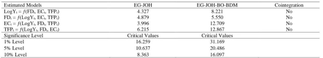
Finally, various Granger causality tests in the selected alternative models suggest unidirectional causality that runs from financial sector development to real income

The empirical analysis that was carried out in this study reveals that in the case of Nigerian economy, there is an evidence of long run relationship between economic

[r]