Bidding structure, market ef
ficiency and persistence in a multi-time
tariff setting
☆
Ezgi Avci-Surucu
a,b,⁎
, A. Kursat Aydogan
a, Doganbey Akgul
ba
Department of Business Administration at Bilkent University, Ankara, Turkey
bMinistry of Energy and Natural Resources, Ankara, Turkey
a b s t r a c t
a r t i c l e i n f o
Article history:
Received 18 February 2015
Received in revised form 20 October 2015 Accepted 27 October 2015
Available online 14 November 2015 JEL classification: C22 C54 D47 Q40 Q48 Keywords:
Restructured electricity prices Fractal noise Long memory Persistence Energy Policies Market Efficiency Bidding Structure
The purpose of this study is to examine the fractal dynamics of day ahead electricity prices by using parametric and semi parametric approaches for each time zone in a multi-time tariff setting in the framework of bidding strategies, market efficiency and persistence of exogenous shocks. We find that that electricity prices have long term correlation structure for thefirst and third time zones indicating that market participants bid hyperbolically and not at their marginal costs, market is not weak form efficient at these hours and exogenous shocks to change the mean level of prices will have permanent effect and be effective. On the other hand, for the second time zone wefind that price series does not exhibit long term memory. This finding suggests the weak form efficiency of the market in these hours and that market participants bid at their marginal costs. Furthermore this indicates that exogenous shocks will have temporary effect on electricity prices in these hours. Thesefindings constitute an important foundation for policy makers and market participants to develop appropriate electricity price forecasting tools, market monitoring indexes and to conduct ex-ante impact assessment.
© 2015 Elsevier B.V. All rights reserved.
1. Introduction
In recent years most electricity markets have been restructured and in this setting, energy-basedfinancial products and electricity price analysis become substantially important for both policy makers and market participants. After the famous California blackout in 2000, a significant increase in the number of studies on price forecasting was observed. Preliminary studies focused on the basic characteristics of electricity differed from those offinancial assets, namely; non-storability, seasonality and inelasticity of supply/demand (Geman and Roncoroni, 2006; Lucia and Schwartz, 2002; Sensfuss et al., 2008; Simonsen et al., 2004; Zachmann, 2008). Following studies focus on spikes, causing asymmetry in the underlying distribution; nonstationarity and mean reversion (Haugom et al., 2011; Janczura et al., 2013; Knittel and Roberts, 2005; Simonsen, 2003; Weron and Przybylowicz, 2000).
Considering security of supply, another crucial feature of electricity is the intraday volatility arising from demandfluctuations during the course of the day. Regulatory authorities usually oblige the system operators to adopt multi-time tariff mechanisms in order to manage peak-time volatili-ty. In these tariff settings, different rates are applied for the consumption at defined time zones during the day. The bills of the subscribers under this setting are arranged by considering their consumptions at the defined time zones and the rates for these time zones with the aim of shifting the load from peak time to off-peak time and thereby enable the end user to manage his energy costs and allow generators to operate efficiently. This situation results in different incentives on generators side. Generators, with the ability offlexible offering, tend to adopt different bidding strategies at super peak, peak and off-peak times.
Studies on analysing dynamics of day ahead prices ignore the different characteristics of time zones in multi-time tariff settings and consider the daily average prices.1However daily average prices do
not capture the microstructure of the day ahead market since level of ☆ It should be noted that the views in this article are entirely those of the authors and do
not represent those of the institutions with which they are affiliated with.
⁎ Corresponding author at: Department of Business Administration at Bilkent University, Ankara, Turkey.
E-mail addresses:[email protected],[email protected](E. Avci-Surucu),
[email protected](A.K. Aydogan),[email protected](D. Akgul).
1
For a comprehensive overview, seeHuisman et al. (2007),Eydeland and Wolyniec (2003)andBunn and Karakatsani (2003).
http://dx.doi.org/10.1016/j.eneco.2015.10.017
0140-9883/© 2015 Elsevier B.V. All rights reserved.
Contents lists available atScienceDirect
Energy Economics
mean reversion and volatility structure are not constant throughout the day (Huisman et al., 2007). Other studies consider hourly prices as a stack and ignore the fact that day ahead electricity prices are determined a day before the trading day for all 24 hours, that is traders cannot update their information set hourly. Under this setting, informa-tion set is not constant throughout the day and updates over the days. Applying a classic time series approach to hourly day ahead prices can be misleading from a statistical point of view.Huisman et al. (2007)
model each hour as a separate time series through a panel data method-ology andfind the mean reversion of day ahead prices is significantly lower over the super-peak hours (18:-22:00). Thus prices are less pre-dictable in these hours. Moreover they show there exists clear blocks of cross-sectional correlation between specific hours. The first block ap-pears in 24:00– 06:00, second block shows up through 6:00 to 19:00 and also there is very high correlation between specific two adjacent hours (between hours 20 and 21; between hours 15 and 16). Thesefindings reveal the different dynamics in hourly prices but similar characteristics in each time zone.
There are also emerging studies of applied mathematics in the field of electricity pricing and market modelling, especially, by the use of game theory, stochastic differential equations and math-ematics supported data mining (Vasin, 2014; Vasin et al., 2013). However the literature on electricity price analysis focuses mostly on the features of autocorrelation, stochasticity and nonlinearity. Only a small number of studies analyse the presence and quanti fi-cation of fractality (long term correlation structure) and very few of them relate thesefindings to basic financial concepts; namely multi-time tariff mechanism, market efficiency, bidding structure or policy development.
Accurate measurement of fractality is crucial for correct statistical inference and forecast uncertainty (Lildholdt, 2000). There are three reasons stimulating this fact. First, ignoring the long memory property in a series can lead to confidence intervals for a process mean that are too optimistic by orders of magnitude. Second, there are many impor-tant economic time series exhibiting long term correlation structure (Beran, 1994). Moreover the potential for spurious regressions of stationary variables depend on the level of fractal noise (Tsay and Chung, 2000).
Economic intuition of the presence of long memory structure in electricity prices is important on several fronts. First, if electricity prices are nonstationary in levels, shocks to electricity prices will have only transitory effects. On the other hand, if electricity prices are stationary, shocks to electricity prices will have permanent effects. The nature of a shock has implications for transmission of that shock from electricity prices to other sectors of the economy. If shocks to electricity prices are permanent, then the probability of transmission of such a shock to other sectors of the economy, where energy prices have a substantial impact on expenditures, would be higher than the probability of transmission of a transitory shock.
Secondly, the presence of fractal noise in electricity prices can be used to capture the bidding strategies of market participants. In restructured electricity markets, the probability of setting the price each hour is not the same for all market participants, mostly because they have different marginal costs. Each hour, the market clearing price is determined by just one generator, called the marginal gener-ator, whose bid is at the intersection of the supply and demand curves. Generators whose bids are higher in the merit order curve are called inframarginal generators. Each generator knows only the past market prices and their own bids. In this setting, the inframarginal generators’ strategy is to not bid higher than the mar-ginal generator’s bid (Sapio, 2004).Thus, they observe and analyse past prices and offer their current bids according to past information. For off-peak hours, if marginal generators bid at their marginal costs, then there is no fractal noise. This observation allows for testing of firms’ bidding behaviour based on marginal cost structures. For peak hours, if there exists a long-term correlation in prices, we can suggest
that marginal generators use the prices of the day and week before, which means applying hyperbolic bidding rules. Moreover this obser-vation is contrary to Fama’s (1970) weak-form efficient market hypothesis (WEMH), which assumes the absence of long-term corre-lation between price increments for any time scale. If markets are weak-form efficient, then market participants cannot earn excess profits in the presence of trading rules based on past prices or returns (Eoma et al., 2008; Farmer et al., 2006; Mun et al., 2008). Such a WEMH can be tested using historical data through short- and long-range correlations (Couillard and Davison, 2005; Lillo and Farmer, 2004).
Thirdly; considering the persistence of a series, the presence and de-gree of long term correlation structure have policy implications.2
Persis-tence is a measure of the speed at which a series returns to its mean level after a shock. In the context of this paper, a shock can be a new policy design/regulation or the introduction of an innovation to the market. In this sense, when the degree of persistence is small, a shock tends to have more temporary effects. In the case of electricity prices, deviating from the mean level of the price is not easy. It is more costly and difficult to permanently affect electricity prices when persistence is low. On the other hand, if the degree of persis-tence is high, a shock tends to have a more long-lasting effect. Thus, the degree of persistence of electricity prices makes a difference in the effectiveness of energy policies/regulations. Therefore results of this study can be an input for regulatory bodies and policy makers to make evidence-based ex-ante policy impact analysis which has re-cently been a popular approach used by UNDP, EU, OECD and World Bank.3
In this paper, our aim is to investigate fractal phenomena in level electricity prices for each time zone separately. We focus on the es-sential statistical properties of fractal noise and identify appropriate instruments for measuring fractality in day ahead electricity prices. Our paper contributes to the literaturefirstly by comprehensively discussing the theoretical characteristics of a fractal pattern and demonstrating the crucial steps of a fractal analysis approach adapted to capture the dynamics of electricity prices. We employ both para-metric and semiparapara-metric methods to benefit from their different statistical properties. Secondly, prior studies have focused on hourly price differences or daily average price differences rather than on level prices. Thisfirst differencing approach is a natural fit for most financial assets because of their nonstationary dynamics. However, this property may not exist for electricity prices depending on the maturity of the market, the time interval, the technology mix and other contaminating factors. For instance; markets with low diversity of generation, low maturity or non-reservoir hydro dependence may experience many spikes which can affect the evaluation of the long memory differencing parameter based on returns. As stated by
Uritskaya and Uritsky (2015)using level prices is more consistent with the original formulation of the parametric long memory estima-tion methods, like DFA. Thus, studies on long memory for level prices can provide useful information to improve existing models and to as-sess limitations on prediction. Lastly, previous studies have investigat-ed either daily average or hourly prices. However,Alvarez-Ramirez and Escarela-Perez (2010)andErzgraber et al. (2008) show that fractal properties of electricity price vary over time. Accordingly we introduce a new time unit based on time zones in a multi-time tariff mechanism considering the fact that electricity market participants have different incentives, risk management and forecasting
2
For details, seeChen and Lee, 2007; Gil-Alana et al., 2010; Peraire and Belbuta, 2012; Apergis and Tsoumas, 2012.
3
For details, seehttp://ec.europa.eu/dgs/energy_transport/evaluation/activites/doc/ reports/energie/intelligent_energy_ex_ante_en.pdf
https://ec.europa.eu/energy/intelligent/files/doc/2011_iee2_programme_ex_ante_en.pdf http://www.oecd.org/dac/povertyreduction/38978856.pdf
http://web.worldbank.org/WBSITE/EXTERNAL/TOPICS/EXTPSIA/0,,contentMDK: 20477296~pagePK:148956~piPK:216618~theSitePK:490130,00.html.
approaches for each time zone. With respect to this fact we expect different levels of predictability of prices, efficiency of the market, bidding structures of market participants and permanence of shocks for each time zone.
For this study we use a data set from Turkey where exists three time zones (Ti); T1(day): 6:00– 17:00, T2(peak): 17:00– 22:00 and T3
(night): 22:00– 6:00. There have been few empirical studies focusing on the statistical and fractal properties of electricity prices in Turkey be-cause of the relative youth of electricity market restructuring. There are only two emerging studies on forecasting electricity prices of Turkey;
Yıldırım et al. (2012)andHayfavi and Talasli (2014). On the other hand Turkey has experienced the longest and most extensive“black out” on 31 March 2015 in the history of the Turkish Republic. This recent experience4has revealed the importance of bidding structures in
elec-tricity markets and implementing hedging strategies. Thus we expect a rapid increase in the number studies on electricity price analysis and forecasting about the Turkish electricity market.
2. Literature review on the fractal dynamics of electricity prices Fractal noise has been found in most scientific fields, including phys-ics,finance, biology and psychology (Chen et al., 1997; Hausdorf and Peng, 1996) and is still a hot topic (Erfani and Samimi, 2009; Barunik and Kristoufek, 2010; Bailie and Morano, 2012; Yerlikaya-Ozkurt et al., 2014; Uritskaya and Uritsky, 2015). It is intermediate between white noise and brown noise and has both stability and adaptability properties (Bak et al., 1987). Different approaches to capture fractality exist. How-ever, statistical characteristics of some nonfractal noise can resemble fractal noise, which may result in incorrect classification. Therefore, proper measurement of fractality in applied research is very difficult. One of the main objectives in measuring fractality is distinguishing be-tween fractal and nonfractal noise for diagnostic checking (Stadnitski, 2012).
Fractality of electricity prices has been the subject of a number of recent studies. Pioneer studies mostly attempt to detect the unit root in a series through analysing the long memory differencing parameter. Some of them use level electricity prices to investigate the unit root in their series and show that the characteristics of electricity prices are very different from those offinancial assets (Atkins and Chen, 2002; De Vany and Walls, 1999; Leon and Rubia, 2001; Rypdal and Lovsleten, 2013); most of them consider the characteristics of the electricity prices similar tofinancial assets and use returns as the main variable in their modelling and their results demonstrate that nonstationarity in electricity prices differs with respect to market and time framework (Norouzzadeh et al., 2007; Simonsen, 2003; Weron, 2002; Weron and Przybylowicz, 2000). Another branch of the literature focus on compar-ing several electricity markets in Europe and US based on their degree of long memory (Alvarez-Ramirez and Escarela-Perez, 2010; Koopman et al., 2007; Koopman et al., 2007; Park et al., 2006) and mainlyfind that the prices are nonstationary and that in some of them fractional differencing exists.
The literature most similar in spirit to ours are the ones focusing on testing basicfinance theories through using long memory correlation structures.Uritskaya and Serletis (2008)compare the market ef ficien-cies in Alberta and Mid-C markets using detrendedfluctuation analysis and spectral exponents.Sapio (2004)finds that long term correlation structure exists in electricity prices and that can be explained by bidding strategies of market participants. He notes that institutional setting is very important in shaping participants’ behaviour and illuminates the relationship between bidding rules and ways of processing past infor-mation. In terms of considering time of the day,Erzgraber et al. (2008)study long-term memory in the Nord Pool market andfind the memory parameter varies greatly with respect to the time of the day. 3. Background
3.1. Deregulated electricity markets
In deregulated electricity markets, there exist different pricing mechanisms. In the context of this paper we consider the uniform price auction in which market participants submit supply and demand curves for each hour where the market clearing price is the equilibrium price. In this type of auction all suppliers and demanders receive and pay the same respective prices. To ensure supply security, there also exists a real-time balancing market. Thus, market participants adopt different bidding strategies according to potential profit opportunities (Dosi and Egidi, 1991; Friedman, 1998; Mazzucato, 2000).
3.2. Electricity market in Turkey
Turkish Day Ahead Electricity Market (GOP) is an emerging spot market which is executed by Market Financial Settlement Centre (PMUM), where generators and demanders submit hourly supply and demand curves and PMUM determines the hourly market clearing price (PTF). GOP was established for ensuring the market participants balancing their portfolio in addition to bilateral contracts and providing the system operator with a balanced system; and is used for power trading and balancing activities one day before the physical delivery of electricity. Participation to the GOP is voluntary. GOP gives permission to hourly, block andflexible bids.
In order to deliver market participants risk-hedging opportunities, trading of electricity future contracts has been launched within the Turkish Derivatives Exchange as of 26 September 2011. Attempts to establish an energy exchange has come up with result and Power Exchange (EPİAŞ) has launched on 1 Sept 2015. EPİAŞ has been operating the day ahead and intraday markets; and Borsaİstanbul (BİST) has the operating right of the derivatives market.
3.3. Propositions
Proposition 1. If marginal generators bid at their marginal costs, then the off-peak price does not display a fractal pattern.
The off-peak hour strategy for generators is to bid at marginal cost (Von der Fehr and Harbord, 1993). If generators use the off-peak strategy and marginal cost is constant, then marginal generators are as-sumed to have no long-term memory since their own cost information is constant. This situation is also an indicator for Fama’s weak-form efficient market hypothesis. If the electricity market is efficient in weak form for each time zone, then prices should not have a long-term correlation structure. Hence, current prices cannot be predicted by using information on past prices.
Proposition 2. If marginal generators use hyperbolic bidding rules, then the peak-load price should be represented by a long memory process and the day ahead market will not be efficient in weak form.
4
Turkey has experienced the longest and most extensive blackout on 31 March 2015 in the history of the Turkish Republic. Turkish Transmission system collapsed for 10 hours due to positioning of generation plants mostly on the eastern part of Turkey. Nevertheless the basic reason is the formation of merit order curve and lack of management initiative. During the winter 2015 Turkey had high precipitation and thus the level of reservoirs be-came very high. On 30 March 2015 , that is the day MOC( Merit Order Curve) was planned for 31 March 2015; the operators recognize that most of the hydro power enter the merit order curve, became marginal generators ( as defined in the manuscript; marginal gener-ators are the ones whose bid at the intersection of the supply and demand curves and thus determining the hourly market clearing price) and natural gas plants mostly located near the Marmara region stay out of the MOC due to their relatively high marginal generation costs. Operators responsible for the realization of the merit order curve ignore the geo-graphical location of the hydro plants and accept / realize the output of the hourly MOCs for the next day to generate electricity at lower prices. On March 31, the electricity trans-mission system collapsed due to the unbalancement in the transtrans-mission lines.
The peak-hour strategy for generators is to bid above marginal cost (Sapio, 2004), since the risk of not being selected is low due to high demand. Thus, at peak load, marginal generators are assumed to give hyperbolically decaying weights to information by considering past electricity prices.
Proposition 3. If shocks to electricity prices are permanent, then the price series for each time zone should exhibit the long memory property.
The presence of fractal patterns in each time zone has important im-plications for public policy design and effectiveness. First, given the strong influence of the energy sector on other sectors of the economy, if shocks to electricity prices are permanent, then such“innovations” may be transmitted to other sectors of the economy as well as to macroeconomic variables. Second, the fractal dynamics of electricity prices are crucial to the design and the effectiveness of public policies. In particular, if electricity prices exhibit long-term correlation structure, then related public policies will tend to have long-lasting effects. In contrast, if electricity prices do not suggest a fractal pattern, then such policies will have only transitory effects (Apergis and Tsoumas, 2012; Gil-Alana et al., 2010; Lean and Smyth, 2009; Pereira and Belbute, 2012).
4. Data
The data used in this study consists of day ahead prices from 00:00 on December 1, 2011 (establishment of the GOP), through 24:00 on April 15, 2014 from the electricity market in Turkey, taken from the Independent Electricity System Operator (TEIAS). This gives us 857 observations for each time zone.
Most studies on analysing fractal dynamics of spot electricity prices take the daily average of hourly prices or returns. We thor-oughly examine this approach by analysing the spectral density of hourly level electricity prices as illustrated inFig. 1 in which the most dominant cycles are observed to be approximately 8, 12, 24 and 48 hours. Thus, we propose to use average price of each time zone i (PTF_Ti) since 1) we do not want to lose information about
the microstructure of day ahead prices, as would be the case were we to use daily averaging 2) previous studies considering each hour separately concludes that there exists a block-structured cross-correlation structure between specific hours referring to the time zones 3) taking average with respect to each time zone is more intuitive in the sense that electricity market participants have different incentives and bidding strategies for each time zone.
Logarithm of PTF_Ti(LNPTF_Ti) are presented in Fig. 2and its
descriptive statistics is illustrated inTable 1.
5. Methodology and results 5.1. Fractal parameters
The main characteristic of a fractal noise is to remain similar when viewed at different scales of time or space. This implies the following statistical properties: 1) a hyperbolically decaying ACF and 2) a specific relation between frequency (f) and size (S) of process variation. Hurst (H), differencing (d), power exponent (β) and scaling exponent (α) are the most commonly used fractal parameters. The Hurst coefficient is the probability that an event in a process is followed by a similar event, which measures the intensity of long-range dependence in a time series.5
Broadly we can classify the differencing parameter estimation methods into two groups; parametric and semiparametric. In the para-metric fractal analysis methods all the parameters are simultaneously estimated mostly through a likelihood function. Within the second group of estimators a periodogram based approach is used (Geweke and Porter-Hudak, 1983; Reisen, 1994; Robinson, 1995).
5.2. Fractal analysis approach
As a general fractal analysis strategy, it is important to remember that none of the fractal parameter estimation procedures mentioned below is superior to the others (Stadnitski, 2012). Simulation studies on fractal analysis have demonstrated that the performance of the var-ious methods depends very much on aspects such as the complexity of the underlying process or the parameterizations (Stadnytska and Werner, 2006). As a result, comprehensive strategies are required to Fig. 1. Raw periodogram of hourly prices from 00:00 on December 1, 2011, to 24:00 on April 15, 2014 with bandwidth 0,000134.
5
It wasfirst introduced byHurst (1951)in hydrological analysis. For both white and brown noises the Hurst coefficient (H) is 0.5; for fractal noise, H = 1. The differencing pa-rameter is another fractal papa-rameter, proposed byGranger and Joyeux (1980)and
Hosking (1981, 1984). They show that if -0.5b d b 0.5, then the process is covariance sta-tionary and the moving average coefficients decay at a relatively slow hyperbolic rate compared with the stationary and invertible autoregresssive moving average (ARMA) process (Bailie et al., 1996). If 0b d b 0.5, then the process is stationary with a finite long memory property. If 0.5≤ d ≤1, then the series is nonstationary (Beran, 1994; Brockwell and Davis, 2002). The power exponent is determined by examining the spectral density function, which describes the amount of variance accounted for by each frequency that can be measured. The analysis of power distribution represents the analysis of variance (ANOVA) in the way that the overall process variance is divided into variance components due to independent cycles of different length (Stadnitski, 2012). If the power spectrum of a set of data is plotted on a log-log scale, the logarithmic power function of fractal noise is expected to follow a straight line with slope -1 for pink noise. The scaling exponent (α) represents the self-similarity of pink noise and fractality can be expressed by the following power low: F (n)∝ nαwithα = 1. If α is 1.5, then the process is brown noise. To
summa-rize, the theoretical parameter values of pink noise are d = 0.5,β = 1, α = 1 and H =1 (Warner, 1998).
correctly estimate fractality parameters. Firstly it is very important to distinguish between stationary and nonstationary processes since some fractal analysis approaches have stationarity assumption or are
more efficient for stationary processes. Traditionally, researchers chose the differencing parameter, d, as an integer (generally 1) to guarantee that the resulting differenced series is a stationary process. In our fractal analysis approach , we propose to check the unit root by a combination of PP and KPSS tests as suggested in (Baillie et al., 1996) and look for in-dication of fractality since unit root tests often lack the power to distin-guish between a truly nonstationary (I(1)) series and a stationary series with a structural break. If the combination of unit root tests indicate fractal behaviour then visual detection methods can be used to ensure the existence of long memory in the data. After getting afirst impression of long memory characteristics of the data visually, one can use appro-priate parametric and semiparametric long memory estimation methods tofind the degree of fractality in the data.
5.2.1. Unit root tests
There are three unit root tests commonly used to test the stationarity of a process: 1) the Augmented Dickey-Fuller (ADF) test, 2) the Phillips– Peron (PP) test and 3) the Kwiatkowski–Phillips–Schmidt–Shin (KPSS) test. ADF (Dickey and Fuller, 1979, 1981) and PP (Phillips, 1987; Phillips and Perron, 1988) test the null hypothesis d = 1 against d = 0. Howev-er,Schwert (1987)noted that when the true generating process is an I(1) process with a large negative moving average coefficient, the Fig. 2. Panel 1: Time series plot of LNPTF_T1from December 1, 2011, to April 15, 2014. Panel 2: Time series plot of LNPTF_T2from December 1, 2011, to April 15, 2014. Panel 3: Time series
plot of LNPTF_T3from December 1, 2011, to April 15, 2014. Note: LNPTF_Tiis the logarithm of average price of time zone i.
Table 1
Descriptive statistics of the data.
LNPTF_T1 LNPTF_T2 LNPTF_T3 # of observ. 867 867 867 Mean 5.095 5.067 4.787 Min 4.029 4.22 3.268 Max 7.06 6.215 5.336 Std. dev. 0.1995 0.1591 0.2491 Skewness 0.277 -0.1777 -1.46 Kurtosis 18.18 8.764 7.742 JB 8330.139*** 1204.967*** 1120.507*** ARCH(10) 389.2607*** 498.3533*** 480.2928*** Q(20) 1433.03*** 3497.096*** 1918.531*** Q2 (20) 1362.056*** 3408.895*** 2087.08** JB is the value of the Jarque-Bera statistic of the price residuals. Q(20) and Q2
(20) are Ljung-Box statistics for the price residuals and the squared price residuals for up to 20th-order serial correlation, respectively. *** indicates rejection of the null hypothesis at the 1% significance level. ** indicates rejection of the null hypothesis at the 5% signifi-cance level. * indicates rejection of the null hypothesis at the 10% signifisignifi-cance level. Note: LNPTF_Tiis the logarithm of average price of time zone i.
performance of the ADF and PP tests is poor, due to their rejecting a unit root too often in favour of an I(0) stationary process. Thus, if we wish to test stationarity as a null and have strong priors in its favour, employing the ADF test may not be useful (Baillie et al., 1996). An empirical series with d close to 0.5 will probably be misclassified as nonstationary. In contrast, the KPSS test assumes that process is stationary (H0: d = 0)
(Kwiatkowski et al., 1992).
Therefore, we use a combination of the PP and KPSS tests allowing us to determine the four possible outcomes of the series (Baillie et al., 1996): 1) if the PP is significant and the KPSS is not, then the data are probably stationary with d∈ (0;0.5)—strong evidence of a covariance stationary process; 2) if the PP is insignificant and the KPSS is significant, then the data may indicate having brown noise—a strong indicator of a unit root, i.e., an I(0) process; 3) if neither the PP nor the KPSS is significant, then the data are insufficiently informative regarding the long memory of the process; and 4) if both the PP and the KPSS are significant, then the data are not well described as either an I(1) or an I(0) process—d ∈ (0; 1).
Table 2presents the unit root tests for logarithm of level prices with-out/with a trend. InTable 2, the p-values pppb0.01 and pKPSSb0.01 are
observed for the analysed series, indicating that the electricity price averages for each time zone are not well described as either an I(1) or an I(0) process which means the differencing parameter, d, is not an integer but between 0 and 1.
5.2.2. Visual detection of long term correlation structure
The second step in our proposed fractal analysis approach is to visually examine the rate of the series’ autocorrelation function and logarithmic power spectrum. For fractal series, we expect a slower hyperbolic decay of autocorrelations in autocorrelation function (ACF) (Beran, 1994).Fig. 3illustrate the ACF of the LNPTF_Tiand
squared-prices for each time zone. There is a slow decay of the autocorrelations, and they are positive and significant even at high lags, which is an indicator of thefinite long memory typical of fractal noise. Only weekly seasonality (lags 7, 14, 28) appears in the data, which means that considering the average price of each time zone eliminates most of the intraday seasonality problem in both level prices and volatility.
Fig. 4presents the autocorrelations offirst differenced price series. After taking thefirst differences of the series, most of the autocorrela-tions at different lags are negative, which is an indicator of over differencing. This plot confirms the observation made above regarding the existence of long term correlation structure in level prices. As a re-sult we use level electricity prices instead offirst differenced prices for the following reasons: 1) the results presented inTable 2,Figs. 3 and 4
provide evidence that the price series do not contain a unit root and would be over differenced if we used thefirst differenced series which is an indicator for fractal behaviour; 2) in a statistical sense, level prices are more informative than differenced prices; 3) in the case of electric-ity, there are in fact no actual returns (as a result offirst differencing) because of the nonstorability of electricity; and 4) the Hurst coefficient might be biased due to the expected antipersistence of the first differenced series.
Fig. 3. Autocorrelation function of LNPTF_Tiand square of LNPTF_Tifor 28 lags Note: LNPTF_Tiis the logarithm of average price of time zone i.
Table 2
Unit root tests for logarithm of level prices with and without a trend.
LNPTF_T1 LNPTF_T2 LNPTF_T3 KPSS (without trend) 0.7402*** 0.4598*** 1*** PP (without trend) -427.7706*** -231.5554*** -240.9871*** KPSS (with trend) 0.1159*** 0.245*** 0.4859*** PP (with trend) -16.37*** -11.59*** -11.96*** *** indicates rejection of the null hypothesis at the 1% significance level. ** indicates rejection of the null hypothesis at the 5% significance level. * indicates rejection of the null hypothesis at the 10% significance level. Note: LNPTF_Tiis the logarithm of average
However, studies show that the sample ACF should not be used as the only visual tool to detect fractality.Agiakoglu and Newbold (1992)
have shown that a substantial part of the slow decaying pattern can originate from the slow rate of convergence of the sample mean. Thus we also use Rescaled range (R/S) and Power spectral density (PSD) anal-yses to ensure the existence of fractality in our data.Mandelbrot and Van Ness (1968)andMandelbrot and Wallis (1969)extended Hurst’s study and proposed R/S analysis. In a log-log R/S plot, if the slope of the straight line is more than 0.5, then the series has a long memory property. If the slope is less than 0.5, the series is antipersistent. R/S sta-tistic can detect long memory in highly non-Gaussian time series with large skewness and kurtosis (Mandelbrot and Wallis, 1969). It has been pointed out byLo, 1991that R/S analysis can be affected by non-stationarities and spurious short-term correlations. In this study we employ the R/S procedure suggested byBeran (1994),Taqqu and Teverovsky (1998)andTaqqu et al. (1995).Fig. 5. illustrates the R/S analysis result of average electricity prices for time zone T2.6
The slopes are far from 0.5, which is an indicator of long memory. To eliminate the sample size problem of R/S analysis, we investigate the electricity price data with least absolute deviation (LAD) regression in-tegrated into the aforementioned procedure to get a robust estimate of the long memory parameter. The results using LAD regression are presented inTable 3and are similar to those of least square (LS) regres-sion. We can conclude that the long memory parameter estimates found by R/S analysis are robust to outliers in the data.
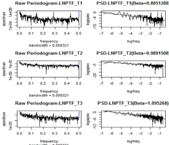
PSD analysis is a periodogram based visualization technique which uses various data transformations such as detrending orfiltering. The
performance of PSD estimators thus depends greatly on the manipulations employed (Delignières et al., 2006; Stadnitski, 2012). If the negative slope is approximately 1 then this is an indicator for long memory. In addition to ACF and R/S, we apply PSD analysis to see if there is a difference between the results of trended and detrended data. The negative slopes (^βPSD) are
nearly 1 for all series. The logarithmic power spectrum of the series is present-ed inFig. 6and seems to be compatible with the long memory property. 5.2.3. Fractal parameter estimation for conditional mean
Lastly, after visual detection of long term correlation structure by ACF, R/S and PSD analysis, we ensure the existence and degree of fractality with respect to each time zone by using parametric and semi-parametric estimation methods. In this paper we estimate the differenc-ing parameter for the conditional mean through Geweke–Porter-Hudak (GPH), Sperio estimator (FDSperio), local Whittle estimator (FDWhittle), Detrended Fluctuation Analysis (DFA) and Autoregressive Fractionally Integrated Moving Average (ARFIMA). We adopt these methods to ben-efit from their different statistical properties; namely GPH’s common usage and comparability with the literature, FDSperio’s usage of smoothed periodogram function instead of spectral density function, FDWhittle’s parametric efficiency and consistency, DFA’s performance for nonstationary series and ARFIMA’s efficiency for series consisting Fig. 5. Rescaled range analysis result of LNPTF_T2Note: LNPTF_T2is the logarithm of average price of time zone 2.
6
Since the appearance of thefigures for the other time zones are similar, they are omit-ted from the text.
Fig. 4. Autocorrelation function offirst differenced LNPTF_Ti. Note: LNPTF_Tiis the logarithm of average price of time zone i.
Table 3
Hurst coefficient estimates using R/S analysis.
LNPTF_T1 LNPTF_T2 LNPTF_T3
R/S estimate with LS 0.7616651 0.8390152 0.8172537 R/S estimate with LAD 0.75644 0.83083 0.8309385 Note: LNPTF_Tiis the logarithm of average price of time zone i.
both long and short memory characteristics. We useTaqqu et al.(1995)’s algorithm to estimate GPH, Reisen (1994) and Taqqu and Teverovsky(1998)algorithms to estimate FDSperio and FDWhittle correspondly. Besides we utilizePeng et al. (1994)’s algorithm to esti-mate DFA and fast and accurate algorithm ofHaslett and Raftery (1989a, 1989b)to estimate d in ARFIMA.
The GPH, the oldest periodogram-based semiparametric estimator, is introduced byGeweke and Porter-Hudak (1983). The GPH estimator is based on the regression equation, using the periodogram function as an estimate of the spectral density (Geweke and Porter-Hudak, 1983; Lobato and Robinson, 1996; Robinson, 1994; Taqqu et al., 1995).
The FDSperio is also a periodogram-based method and was proposed in order to improve the GPH estimator. It takes advantage of theReisen (1994)algorithm to estimate the fractal parameter d in the ARFIMA (p,d,q) model. It is based on the regression equation, using the smoothed periodogram function as an estimate of the spectral density. The FDWhittle is one of the most commonly used parametric periodogram-based Whittle estimators. It was proposed byWhittle (1953)
and modified by Künsch (1987), Robinson (1995b) and Taqqu and Teverovsky (1998). One of the advances of the Whittle Estimator is that it is consistent and asymtotically normal for nonstationary and unit root cases (Phillips and Shimotsu, 2004). Whittle's methodfits the parameters of a spec-ified spectral density function(SDF) model to data by optimizing an appropri-ate function using an estimappropri-ate of the SDF for an input time series.
Another method we use to detect long memory is DFA which was proposed byPeng et al. (1994)based on the relationship F(n)∝ nα.
DFA analysis performs better for detecting the long memory property in nonstationary series.7Hu et al. (2001)focus on the effect of trends
on DFA, whileKristoufek (2010)examinesfinite sample properties
and confidence intervals of DFA. In DFA, if there is a straight line with slope 0.5, then the series is white noise. If the slope is greater than 0.5, then the series is persistent. If the slope is less than 0.5, then the series is antipersistent. We apply the DFA estimator on both the trended and detrended data to investigate the effects of trends on detecting long memory.
ARFIMA is the most frequently used parametric method with the ability to estimate the short- and long-memory parameters jointly (Reisen et al., 2001; Sowell, 1992b). Its main disadvantages are that it is valid only for stationary series and needs a sufficiently large sample size for acceptable measurement accuracy (Stadnitski, 2012; Stadnytska and Werner, 2006). Its validness only for stationary series can lead to situations where nonstationary processes are classified as having long memory. The exact maximum likelihood (EML) method introduced by
Sowell (1992a), the conditional sum of squares (CSS) approach pro-posed by Chung (1996) and the approximate method likelihood (AML) method introduced byHaslett and Raftery (1989a, 1989b)are commonly used to estimate the fractional differencing parameter in ARFIMA models.
Semiparametric estimates (PSD, DFA and HurstSpec) are convert-ed to d̂ to make the comparison of results clearer, and illustrated in
Table 4. The estimates range from 0.4 to 0.7 depending on the tariff zone, except for those of the DFA. The interpretation of fractal dynamics is clearer for time zones T1and T3since the range of the
parameters is between 0.4 and 0.6 for most of the estimators. Howev-er, the fractal estimates for time zone T2are in the critical region
between fractional integration and nonstationarity. We take thefirst difference of the T2series for the sake of eliminating the potential
nonstationarity in that series. As illustrated inTable 5, the T2series
does not exhibit long memory after taking the first difference, which indicates that electricity prices in time zone T2do not have
long memory.
7
SeeGrech and Mazur (2005)for a discussion of the statistical properties of old and new techniques in detrendedfluctuation analysis of time series.
The deficiency of the semiparametric methods is to overestimate fractality in time series that contain both long- and short-range compo-nents. Due to larger biases, the precision of semiparametric methods is distinctly inferior to that of the ARFIMA approaches. Since the values ob-tained for T1and T3are all smaller than 0.6, the preceding analyses do
not allow rejecting the hypothesis of fractality for the T1and T3series.
Therefore, ARFIMA analysis appears to be appropriate for the T1and T3
series. The comparison of different ARFIMA models is analysed using Akaike information criteria (AIC); a summary of the results is presented inTable 6. T1and T3exhibit the long-term memory property using
models ARFIMA (0, 0.4090, 0) and ARFIMA (1, 0.3202, 0) respectively. In summary, the time zones defined in the multi-time tariff mechanism are found to have different fractal dynamics.
5.2.4. Fractal parameter estimation for conditional variance
Studies byDe Lima and Crato (1994),Ding et al. (1993)andHarvey (1993)all reported the apparent presence of long memory in the auto-correlations of squared returns of variousfinancial asset prices. Long memory in volatility is an indicator of uncertainty and risk (Barkoulas et al., 2000; Kasman and Torun, 2007; Kasman et al., 2009; Ural and Kücüközmen, 2011). There are different approaches to measure the long memory in volatility. Some of the previous studies use the square of the returns of assets as an artificial variable and apply semiparametric methods to this variable tofind the fractal parameter for process volatility. However, as noted byWright (2002), the fractal parameter d is underestimated when using this approach. Thus we use the para-metric fractionally integrated generalized autoregressive conditionally heteroskedastic (FIGARCH) estimator introduced by Baillie et al. (1996)to eliminate the deficiency of using square of the returns. Estimation results are illustrated inTable 7. Among the FIGARCH models, we chose for consideration the one with the lowest AIC. The volatility of T1and T2does not seem to exhibit long memory with
signif-icant (approximately 1) d estimates, which indicates that there is an I(1) process in volatility and that the T3series has a long memory
property in volatility. 6. Concluding Remarks
We empirically investigate three propositions considering the presence of long-term correlation in day ahead electricity prices for each time zone in a multi-time tariff setting. The results obtained
provide new information on the fractal behaviour of electricity prices considering different time zones. We have reached the following main conclusions:
6.1. Analysing the fractal dynamics of electricity prices is very complicated because of the unique characteristics of electricity, and requires elaborate strategies
Numerous procedures have been developed for estimating the fractal parametersβ, α, H and d. Approaches aimed at detecting long memory in the conditional mean and variance have been developed in-dependently of each other; however, long-term correlation structure is often observed in both the conditional mean and variance. Thus, we investigated the presence of the long memory property in both the conditional mean and variance for each time zone. Moreover the crucial steps of a fractal analysis approach customized to capture electricity price dynamics are demonstrated elaborately.
6.2. Considering time zones in electricity price analysis is very intuitive and important
Our results suggest that the fractal dynamics of electricity prices are different for each time zone. Long-memory parameters are found to be significantly different from zero for the conditional mean, indicating long-term dependence for time zone 1. This confirms the proposition that at peak load, marginal generators may give hyperbolically decaying weights to information by considering the prices of a day/week before. We also show that the T3price series has a long memory property in
both level and volatility. T2price series, however, does not have long
memory in either level or volatility. It is nonstationary but mean reverting.
6.3. Implications of the propositions can be different for each time zone Positive and significant fractional differencing coefficients of the mean for the T1series suggest that marginal generators exhibit hyperbolic Table 5
Long memory tests for diff-LNPTF_T2prices in converted measures.
LM MEASURES
Vrb. DFA FDSperio FDGPH FDWhittle HurstSpec ModR/S
DIFF_LNPTF_T2 Pt 0.1181902 -0.2073319 -0.3668577 -0.4716051 -0.3855214 1.0462
Notes: DIFF_LNPTF_T2 is thefirst differenced LNPTF_T2. LNPTF_Tiis the logarithm of average price of time zone i.
Table 4
Long memory tests for log prices in converted measures. LM MEASURES
Vrb. DFA FDSperio FDGPH FDWhittle HurstSpec ModR/S LNPTF_T1 Pt 0.5278 0.4692 0.5020 0.4145 0.5991 1.9054* Pt2 0.5199 0.4569 0.4983 0.3959 0.5929 1.9164* LNPTF_T2 Pt 0.6893 0.6675 0.5292 0.5240 0.5956 1.8218 Pt2 0.6846 1.1847 0.5341 0.5140 0.6020 1.8141 LNPTF_T3 Pt 0.5652 0.4489 0.4991 0.5643 0.5756 2.2477** Pt2 0.5788 0.4637 0.5203 0.5725 0.5876 2.2541**
*** indicates rejection of the null hypothesis at the 1% significance level. ** indicates rejec-tion of the null hypothesis at the 5% significance level. * indicates rejecrejec-tion of the null hy-pothesis at the 10% significance level. Note: LNPTF_Tiis the logarithm of average price of
time zone i.
Table 6
Estimation results of the ARFIMA models. LNPTF_T1 (0,ξ, 0) LNPTF_T3 (1,ξ, 0) μ 5.083 4.7942 α1 - 0.3310 ξ 0.4090*** 0.3202*** ln(L) 361.7459 292.3939 AIC -716.7280 -571.2623 Skewness 0.3864 -1.162 Kurtosis 24.83 8.649 JB 17214.27*** 1345.054*** Q(20) 305.0713*** 106.1891*** Q2(20) 114.704*** 83.5265*** ARCH(10) 95.7151*** 70.3495***
Notes:μ is the time series mean. ξ is the fractional differencing parameter. ln(L) is the value of the maximized Gaussian likelihood. JB is the value of the Jarque-Bera statistic of the price residuals. Q (20) and Q2
(20) are Ljung-Box statistics for the price residuals and the squared price residuals for up to 20th-order serial correlation, respectively. *** indi-cates rejection of the null hypothesis at the 1% significance level. ** indiindi-cates rejection of the null hypothesis at the 5% significance level. * indicates rejection of the null hypothesis at the 10% significance level. LNPTF_Tiis the logarithm of average price of time zone i.
information processing, which supports Proposition 1. Further, since there exists long-term correlation structure, future prices are predictable from past prices, and the market is not efficient in weak form in the T1
time zone. This structure also indicates that exogenous shocks/innova-tions can have permanent effects on prices. Thus, the effectiveness of price policies for T1is expected to be high.
Interpretation of the long-term correlation structure is different for the T3time zone, where the demand for and price of electricity is low.
In this time zone, only the base load power plants (thermal, hydroelec-tric plants without dams, and renewable) offer to the market. To rank along the merit order curve, base load power plants are expected to offer at their marginal costs. Since demand is uncertain, participants face a trade-off between submitting a high but risky bid, and a safer but potentially less profitable low bid. If marginal generators bid at their marginal costs, they are expected not to bid hyperbolically and not to have long memory. However, wefind that off-peak fractional differencing coefficients are significantly greater than zero, which can be taken as evidence that bidding above marginal cost occurs even off-peak. Thisfinding further suggests that the market is not efficient in weak form and that future prices are predictable from past prices. Moreover, exogenous shocks can have permanent effects on prices.
T2is the peak-load time zone, where demand is very high and the
probability of not being on the merit order curve is very low, even for high bids. Thus, at peak load, marginal generators would be expected to give hyperbolically decaying weights to information by considering the prices of a day/week before. However, ourfindings suggest that the T2price series does not display a long memory property in either
level prices or volatility. Thisfinding suggests that marginal generators do not consider past information in their bidding processes and offer at their marginal costs. Further, since long-term correlation structure does not exist, future prices are not predictable from past prices, and the market is weak-form efficient in T2. Thisfinding also indicates that
innovations to the market can have temporary effect for the T2time
zone.
6.4. Suggestions for future research
Developing approaches more robust to skewed distributions for the conditional mean would provide an opportunity on relaxing the normality assumption. Developing new electricity market monitoring indexes considering the time zones would result in interesting policy
implications. Furthermore considering the fractal dynamics of electricity prices at different time scales, one would reduce the prediction con fi-dence intervals.
Appendix A. Supplementary data
Supplementary data to this article can be found online athttp://dx. doi.org/10.1016/j.eneco.2015.10.017.
References
Agiakoglu, C., Newbold, P., 1992.Empirical Evidence on Dickey–Fuller Type Tests. J. Time Ser. Anal. 13, 471–483.
Alvarez-Ramirez, J., Escarela-Perez, R., 2010.Time-dependent correlations in electricity markets. Energy Econ. 32, 269–277.
Apergis, N., Tsoumas, C., 2012.Long memory and disaggregated energy consumption: ev-idence from fossil fuels, coal and electricity retail in the US. Energy Econ. 34, 1082–1087.
Atkins, F.J., Chen, J., 2002.Some statistical properties of deregulated electricity prices in Alberta. Discussion paper. University of Calgary.
Baillie, R.T., 1996.Long memory processes and fractional integration in econometrics. J. Econ. 73, 5–59.
Bailie, R.T., Morana, C., 2012.Adaptive ARFIMA models with applications to inflation. Econ. Model. 29, 2451–2459.
Baillie, R.T., Bollerslev, T., Mikkelsen, H.O., 1996.Fractionally integrated generalized autoregressive conditional heteroskedasticity. J. Econ. 74, 3–30.
Bak, P., Tang, C., Wiesenfeld, K., 1987.Self-organized criticality: an explanation of 1/f noise. Phys. Rev. Lett. 59, 381–384.
Barkoulas, J.T., Baum, C.F., Travlos, N., 2000.Long Memory in the Greek Stock Market. Appl. Financ. Econ. 10, 177–184.
Barunik, J., Kristoufek, L., 2010.On Hurst exponent estimation under heavy tailed distributions. Appl. Phys. A 389, 3844–3855.
Beran, J., 1994.Statistics for Long-Memory Processes. Monographs on Statistics and Applied Probability vol. 61. Chapman and Hall, New York.
Brockwell, P.J., Davis, R.A., 2002.Introduction to Time Series and Forecasting. Springer, New York.
Bunn, D.W., Karakatsani, N., 2003.Forecasting electricity prices. Working paper. London Business School.
Chen, P.-F., Lee, C.-C., 2007.Is Energy Consumption Per Capita Broken Stationary? New Evidence from Regional-Based Panels. Energy Policy 35 (6), 3526–3540.
Chen, Y., Ding, M., Kelso, J.A.S., 1997.Long memory processes (1/fa type) in human coordination. Phys. Rev. Lett. 79, 4501–4504.
Chung, C.F., 1996.A generalized fractionally integrated ARMA process. J. Time Ser. Anal. 2, 111–140.
Couillard, M., Davison, M., 2005.A comment on measuring the Hurst exponent of financial time series. Appl. Phys. A 348, 404–418.
De Lima, P.J.F., Crato, N., 1994.Long-range dependence on the conditional variance of stock returns. Econ. Lett. 45 (3), 281–285.
De Vany, A., Walls, W., 1999.Cointegration analysis of spot electricity prices. Insights on transmission efficiency in the Western US. Energy Econ. 21, 435–488.
Delignières, D., Ramdani, S., Lemoine, L., Torre, K., 2006.Fractal analyses for short time series: a re-assessment of classical methods. J. Math. Psychol. 50, 525–544.
Dickey, D., Fuller, W., 1979.Distribution of the estimators for autoregressive time series with a unit root. J. Am. Stat. Assoc. 74, 427–431.
Dickey, D.A., Fuller, W.A., 1981.Likelihood Ratio Statistics for Autoregressive Time Series with a Unit Root. Econometrica 49, 4.
Ding, Z., Granger, C.W.J., Engle, R.F., 1993.A long memory property of stock market returns and a new model. J. Empir. Financ. 1, 83–106.
Dosi, G., Egidi, M., 1991.Substantive and Procedural Uncertainty: An Exploration of Economic Behaviours in Changing Environments. J. Evol. Econ. 1 (2), 145–168.
Eoma, C., Choi, S., Oh, G., Jung, W.S., 2008.Hurst Exponent and Prediction Based on Weak-form Efficient Market Hypothesis of Stock Markets. Appl. Phys. A 387, 4630–4636.
Erfani, A., Samimi, A.J., 2009.Long memory forecasting of stock price index using a frac-tionally differenced ARMA model. J. Appl. Sci. Res.
Erzgraber, H., Strozzi, F., Zaldivar, J.-M., Touchette, H., Gutierrez, E., Arrowsmith, D., 2008.
Time series analysis and long range correlations of Nordic spot electricity market data. Appl. Phys. A 387, 6567–6574.
Eydeland, A., Wolyniec, K., 2003.Energy and Power Risk Management. Wiley.
Fama, E., 1970.Efficient capital markets: A review of theory and empirical work. J. Financ. 25, 383–417.
Farmer, J.D., Gerig, A., Lillo, F., Mike, S., 2006.Market efficiency and the long-memory of supply and demand: is price impact variable and permanent orfixed and temporary? Rev. Quant. Finan. Acc. 6 (2), 107–112.
Friedman, D., 1998.Evolutionary economics goes mainstream: A review of the theory of learning in games. J. Evol. Econ. 8 (4), 423–432.
Geman, H., Roncoroni, A., 2006.Understanding thefine structure of electricity prices. J. Bus. 79 (3), 1225–1261.
Geweke, J., Porter-Hudak, S., 1983.The estimation and application of long memory time series models. J. Time Ser. Anal. 4 (4), 221–238.
Gil-Alana, L.A., Loomis, D., Payne, e J., 2010.Does Energy Consumption by the US Electric Power Sector Exhibit Long Memory Behavior? Energy Policy 38, 7515–7518.
Granger, C.W.J., Joyeux, R., 1980.An introduction to long-memory time series and fractional differencing. J. Time Ser. Anal. 1 (1), 15–29.
Table 7
Estimation results of the FIGARCH models.
LNPTF_T1 LNPTF_T2 LNPTF_T3 FIGARCH (1,d,0) FIGARCH (1,d,0) FIGARCH (1,d,1) μ = C 5.1150*** 5.1043*** 4.8463*** ω = A 0.0099*** 0.0038*** 0.0077*** α1 -0.1427*** -0.1626*** 0.1183*** β1 - - 0.5209*** d 0.9905*** 0.9496*** 0.4772*** ln(L) 378.39 581.95 170.94 AIC -748.798 -1155.913 -331.8805 BIC -729.7378 -1136.853 -308.0553 Skewness -0.7593 -0.5102 -0.8601 Kurtosis 5.652 7.274 5.615 JB 337.3517*** 697.3718*** 353.96*** Q(20) 1026.547*** 1689.58*** 956.45*** Q2 (20) 188.5044*** 8.1472 15.2484 ARCH(10) 84.6719*** 3.3638 5.9687 Notes:μ is the time series mean. d is the fractional differencing parameter. ln(L) is the value of the maximized Gaussian likelihood. JB is the value of the Jarque-Bera statistic of the price residuals. Q (20) and Q2
(20) are Ljung-Box statistics for the price residuals and the squared price residuals for up to 20th-order serial correlation, respectively. *** indi-cates rejection of the null hypothesis at the 1% significance level. ** indiindi-cates rejection of the null hypothesis at the 5% significance level. * indicates rejection of the null hypothesis at the 10% significance level. LNPTF_Tiis the logarithm of average price of time zone i.
Grech, D., Mazur, Z., 2005.Statistical properties of old and new techniques in detrended analysis of time series. Acta Phys. Pol. B 36, 2403–2413.
Harvey, A.C., 1993.Time Series Models. Second edition. MIT Press, Massachusetts.
Haslett, J., Raftery, A.E., 1989a.Space-time modelling with long-memory dependence: assessing Ireland’s wind power resource. Appl. Stat. 38, 1–50.
Haslett, J., Raftery, A.E., 1989b.Space-time Modelling with Long-memory Dependence: Assessing Ireland's Wind Power Resource (with Discussion). Appl. Stat. 38, 1–50.
Haugom, E., Westgaard, S., Solibakke, P.B., Lien, G., 2011.Realized volatility and the influ-ence of market measures on predictability: Analysis of Nord Pool forward electricity prices. Energy Econ. 33, 1206–1215.
Hausdorf, J.M., Peng, C.K., 1996.Multiscaled randomness: a possible source of 1/f noise in biology. Phys. Rev. E Stat. Phys. Plasmas Fluids Relat. Interdiscip. Topics 54, 2154–2157.
Hayfavi, A., Talasli,İ., 2014.Stochastic multifactor modeling of spot electricity prices. Comput. Appl. Stat. 259, 434–442.
Hosking, J.R.M., 1981.Fractional differencing. Biometrika 68, 165–176.
Hosking, J.R.M., 1984.Modelling persistence in hydrological time series using fractional differencing. Water Resour. Res. 20, 1898–1908.
Hu, K., Ivanov, P., Chen, Z., Carpena, P., Stanley, H., 2001.Effect of trends on detrended fluctuation analysis. Phys. Rev. E 64 (art. 011114).
Huisman, R., Huurman, C., Mahieu, 2007.Hourly electricity prices in day-ahead markets. Energy Econ. 29, 240–248.
Hurst, H., 1951.Long-term storage capacity of reservoirs. Trans. Am. Soc. Agric. Eng. 116, 770–799.
Janczura, J., Trueck, S., Weron, R., Wolff, R.C., 2013.Identifying spikes and seasonal components in electricity spot price data: A guide to robust modeling. Energy Econ. 38, 96–110.
Kasman, A., Torun, E., 2007.Long Memory in the Turkish Stock Market Return and Volatility. Cent. Bank Rev. 2, 13–27.
Kasman, A., Kasman, S., Torun, E., 2009.Dual Long Memory Property in Returns and Volatility: Evidence from the CEE Countries’ Stock Markets. Emerg. Mark. Rev. 10, 122–139.
Knittel, C.R., Roberts, M.R., 2005.An empirical examination of restructured electricity prices. Energy Econ. 27 (5), 791–817.
Koopman, S.J., Ooms, M., Carnero, M.A., 2007.Periodic seasonal Reg-Arfima–Garch models for Daily electricity spot prices. J. Am. Stat. Assoc. 102 (477), 16–27.
Kristoufek, L., 2010.Rescaled range analysis and detrendedfluctuation analysis: Finite sample properties and confidence intervals. AUCO Czech Econ. Rev. 4 (3), 236–250.
Künsch, H., 1987.Statistical aspects of self-similar processes. Proceedings of the First World Congress of the Bernoulli Society 1, pp. 67–74.
Kwiatkowski, D., Phillips, P., Schmidt, P., Shin, Y., 1992.Testing the null of stationarity against alternative of a unit root: How sure are we that the economic time series have a unit root? J. Econ. 54, 159–178.
Lean, H., Smyth, R., 2009.Long memory in US disaggregated petroleum consumption: Evidence from univariate and multivariate LM tests for fractional integration. Energy Policy 37, 3205–3211.
Leon, A., Rubia, A., 2001.Comportamiento del Precio y Volatilidad en el Pool Eléctrico Español. Instituto Valenciano de Investig, pp. 2001–2004.
Lildholdt, P., 2000.Long Memory and ARFIMA Modelling of Inflation Rates (MSc Dissertation) Department of Economics, University of Aarhus.
Lillo, F., Farmer, J.D., 2004.The Long Memory of the Efficient Market. Stud. Nonlinear Dyn. Econom. 8 (3), 1–35.
Lo, A.W., 1991.Long-term memory in stock market prices. Econometrica 59, 1279–1313.
Lobato, I., Robinson, P.M., 1996.Averaged periodogram estimation of long memory. J. Econ. 73, 303–324.
Lucia, J.J., Schwartz, E.S., 2002.Electricity prices and power derivatives: Evidence from the Nordic power exchange. Rev. Deriv. Res. 5 (1), 5–50.
Mandelbrot, B., van Ness, J., 1968.Fractional Brownian motions, fractional noises and applications. SIAM Rev. 10 (422), 422–437.
Mandelbrot, B.B., Wallis, J.R., 1969.Some Long-Run Properties of Geophysical Records. Water Resour. Res. 5 (2), 321–340.
Mazzucato, M., 2000.Firm Size, Innovation and Market Structure: The Evolution of Market Concentration and Instability. Northampton, MA, Edward Elgar 1-84064-346-3, p. 138.
Mun, H.W., Sundaram, L., Yin, O.S., 2008.Leverage Effect and Market Efficiency of Kuala Lumpur Composite Index. Int. J. Bus. Manag. 3 (4), 138–144.
Norouzzadeh, P., Dullaert, W., Rahmani, B., 2007.Anti-correlation and multifractal features of Spain electricity spot market. Appl. Phys. A 380, 333–342.
Park, H., Mjelde, J.W., Bessler, D.A., 2006.Price dynamics among U.S. electricity spot mar-kets. Energy Econ. 28, 81–101.
Peng, C., Buldyrev, S., Goldberger, A., Havlin, S., Simons, M., Stanley, H.E., 1994.Mosaic or-ganization of DNA nucleotides. Phys. Rev. E 49 (2), 1685–1689.
Pereira, A.M., Belbute, J.M., 2012.Final energy demand in Portugal: how persistent it is and why it matters for environmental policy. CEFAGE-UE Working Paper 2011/20.
Phillips, P.C.B., 1987.Time series regression with a unit root. Econometrica 55, 277–301.
Phillips, P.C.B., Perron, P., 1988.Testing for a unit root in time series regression. Biometrika 75, 335–346.
Phillips, P.C.B., Shimotsu, K., 2004.Local whittle estimation in nonstationary and unit root cases. Ann. Stat. 32 (2), 659–692.
Reisen, V., 1994.Estimation of the fractional difference parameter in the ARFIMA (p, q, d) model using the smoothed periodogram. J. Time Ser. Anal. 15, 335–350.
Reisen, V., Abraham, B., Toscano, E., 2001.Parametric and semiparametric estimations of stationary univariate ARFIMA models. Braz. J. Probab. Stat. 14, 185–206.
Robinson, P.M., 1994.Semiparametric analysis of long-memory time series. Ann. Stat. 22, 515–539.
Robinson, P.M., 1995.Log-Periodogram Regression of Time Series with Long Range Dependence. Ann. Stat. 23 (3), 1048–1072.
Rypdal, M., Lovsleten, O., 2013.Modeling electricity spot prices using mean-reverting multifractal processes. Appl. Phys. A 392, 194–207.
Sapio, S., 2004.Markets Design, Bidding Rules, and Long Memory in Electricity Prices. Revue deconomie Industrielle, Programme National Perse. 107(1), pp. 151–170
Schwert, G.W., 1987.Effects of model specification on tests for unit roots in macroeco-nomic data. J. Monet. Econ. 20, 73–103.
Sensfuss, F., Ragwitz, M., Genoese, M., 2008.The merit-order effect: A detailed analysis of the price effect of renewable electricity generation on spot market prices in Germany. Energy Policy 36 (8), 3086–3094.
Simonsen, I., 2003.Measuring anti-correlations in the Nordic electricity spot market by wavelets. Appl. Phys. A 322, 597–606.
Simonsen, I., Weron, R., Mo, B., 2004.Structure and stylized facts of a deregulated power market. MPRA Paper. 1443, pp. 1–29.
Sowell, F., 1992a.Maximum likelihood estimation of stationary univariate fractionally in-tegrated time series models. J. Econ. 53, 165–188.
Sowell, F., 1992b.Modeling long-run behavior with the fractional ARFIMA model. J. Monet. Econ. 29, 277–302.
Stadnitski, T., 2012.Measuring Fractality. Front. Physiol. 3, 27.
Stadnytska, T., Werner, J., 2006.Sample size and accuracy of estimation of the fractional differencing parameter. Methodology 4, 135–144.
Taqqu, M.S., Teverovsky, W., 1998.On Estimating the Intensity of Long- Range Depen-dence in Finite and Infinite Variance Time Series in A practical Guide to Heavy Tails. Statistical Techniques and Applications. Birkhauser, Boston, pp. 177–217.
Taqqu, M., Teverosky, W., Willinger, W., 1995.Estimators for long-range dependence: an empirical study. Fractals 3 (4), 785–798.
Tsay, W.-J., Chung, C.-F., 2000.The spurious regression of fractionally integrated process-es. J. Econ. 96, 155–182.
Ural, M., Kücüközmen, C.C., 2011.Analyzing the dual long memory in stock market returns. Ege Academic Review. 11, pp. 19–28
Uritskaya, O.Y., Serletis, A., 2008.Quantiftying multiscale efficiency in electricity markets. Energy Econ. 30 (6), 3109–3117.
Uritskaya, O.Y., Uritsky, V.M., 2015.Predictability of price movements in deregulated elec-tricity markets. Energy Econ. 49, 72–81.
Vasin, A., 2014.Game-theoretic Study of Electricity Market Mechanisms. Procedia Comput. Sci. 31 (2014), 124–132.
Vasin, A., Kartunova, P., Weber, G.-W., 2013.Models for Capacity and Electricity Market Design. CEJOR 21 (3), 651–661.
Von der Fehr, N., Harbord, D., 1993.Spot market competition in the UK electricity industry. Econ. J. 103 (418), 531–546.
Warner, R.M., 1998.Spectral analysis of time- series data. Guilford, New York.
Weron, R., 2002.Estimating long range dependence:finite sample properties and confidence intervals. Appl. Phys. A 312 (1), 285–299.
Weron, R., Przybylowicz, B., 2000.Hurst analysis of electricity price dynamics. Appl. Phys. A 283, 462–468.
Whittle, P., 1953.Estimation and information in stationary time series. Ark. Mat. 2, 423–434.
Wright, J.H., 2002.Log-periodogram estimation of long memory volatility dependencies with conditionally heavy tailed returns. Econ. Rev. 21, 397–417.
Yerlikaya-Ozkurt, F., Vardar-Acar, C., Yolcu-Okur, Y., Weber, G.-W., 2014.Estimation of the Hurst parameter for fractional Brownian motion using the CMARS method. J. Comput. Appl. Math. 259, 843–850.
Yıldırım, M.H., Ozmen, A., Türker-Bayrak, Ö., Weber, G.-W., 2012.Electricity price modelling for Turkey. Operations Research Proceedings.
Zachmann, G., 2008.Electricity wholesale market prices in Europe: Convergence? Energy Econ. 30 (4), 1659–1671.