Linear Passive Networks With Ideal Switches:
Consistent Initial Conditions and State Discontinuities
Roberto Frasca, M. Kanat Camlibel, Member, IEEE, I. Cem Goknar, Fellow, IEEE, Luigi Iannelli, Member, IEEE,
and Francesco Vasca, Member, IEEE
Abstract—This paper studies linear passive electrical networks with ideal switches. We employ the so-called linear switched sys-tems framework in which these circuits can be analyzed for any given switch configuration. After providing a complete characteri-zation of admissible inputs and consistent initial states with respect to a switch configuration, the paper introduces a new state reini-tialization rule that is based on energy minimization at the time of switching. This new rule is proven to be equivalent to the classical methods of Laplace transform and charge/flux conservation prin-ciple. Also we illustrate the new rule on typical examples that have been treated in the literature.
Index Terms—Consistent initial conditions, energy-based jump rule, state discontinuities, state jump, switched networks.
I. INTRODUCTION
S
WITCHING circuits are encountered in various appli-cations from power converters to signal processing. To simplify the analysis, the switching elements are typically taken as ideal elements. Such ideal switching behavior may cause discontinuities in the state variables (typically voltages across capacitors and currents through inductors). A good deal of literature on switched networks has been devoted to the problem of state reinitialization, i.e., determining the state after a discontinuity. The main goal of this paper is to study the state reinitilization problem for electrical networks consisting of linear passive elements, independent voltage/current sources, and ideal switches.For an account of previous work in the literature, we give the following inevitably incomplete survey of related work within the area of circuit theory. In the classical book [1], state reinitilization problem has been addressed by utilizing the charge/flux conservation principle. A general formalization of this conservation principle has not been given; it has been explained only through examples. A set of algebraic equations was obtained in [2] for reinitilization of active RLC circuits. In case of a passive network, the method reduces to the applica-tion of charge/flux conservaapplica-tion principle. In [3], the principle of charge/flux conservation has been applied to periodically operated switched networks for state reinitilization problem. In [4], the authors proposed a reinitilization method that is based
Manuscript received July 29, 2009; revised January 09, 2010 and March 24, 2010; accepted April 24, 2010. Date of publication August 03, 2010; date of current version December 15, 2010. This paper was recommended by Associate Editor E. Alarcon.
R. Frasca, L. Iannelli, and F. Vasca are with the Department of Engineering, University of Sannio, Benevento, Italy (e-mail: [email protected]; [email protected]; [email protected]).
M. K. Camlibel is with the Johan Bernoulli Institute of Mathematics and Computer Science, University of Groningen, The Netherlands. He is also with the Department of Electronics and Communications Engineering, Dogus Uni-versity, Istanbul, Turkey (e-mail: [email protected]).
I. C. Goknar is with the Department of Electronics and Communications En-gineering, Dogus University, Istanbul, Turkey (e-mail: [email protected]).
Digital Object Identifier 10.1109/TCSI.2010.2052511
on numerical inversion of Laplace transform. Their method obtains consistent initial states in two steps: one step forward in time to overcome the impulse and one step backward to the switching instant. Reference [5] uses also the Laplace transform method for reinitilization. This line of work has been extended in [6] to periodically switched nonlinear circuits. Other papers that took numerical approaches include [7]–[9]. The distribu-tional framework has been used in [10] where current sources were excluded, in [11] an approach to calculate the energy loss after the discontinuity was developed. Other related work consists of generalizations to nonlinear setting (e.g., [12]–[15]) and calculation and interpretation of energy loss in switching instants (e.g., [16]–[18]). For internally controlled switching elements, state reinitialization was considered in [19]–[22]. Also state discontinuities were discussed in the context of switched capacitor circuits in [23], [24], in the context of robust stabilization of complex switched networks in [25], and in the context of steady-state analysis of nonlinear circuits containing ideal switches in [26]. In the literature, switched networks have been almost always treated by fixing a switch configuration and deriving the differential algebraic equations that govern the network. In order to analyze the same circuit for another switch configuration, a typical approach consists of deriving the corresponding circuit equations for the new configuration (see, e.g., [8]). In our work, we employ the so-called linear
switched systems framework (see, e.g., [21], [27]) that allows
one to obtain circuit equations for any switch configuration in a natural way. Within this framework, we assume that the network elements other than the ideal switches and sources are linear and passive. Based on this assumption, we give a complete characterization (for any given switch configuration) of admissible inputs (voltage/current sources), i.e., sources that are acceptable and consistent initial states, i.e., initial states that do not cause discontinuities in the state variable. After that, we study the inconsistent initial states, i.e., initial states that cause discontinuities. First, we introduce an energy-based
jump rule for determining the state after a jump occurs. The
novelty of this new rule stems from its conceptual insight and computational simplicity. Finally, the other two alternative methods for determining the state after discontinuity, namely Laplace transform method and charge/flux conservation prin-ciple have been investigated. We show that these two methods are equivalent to the new energy-based jump rule.
The structure of the paper is as follows. After introducing the notational conventions in Section II, we begin with setting a general framework for linear switched systems in Section III. This is followed by a quick review of the notion of passivity in Section IV. In Section V, a complete characterization of ad-missible inputs and consistent initial states is presented. For the inconsistent states, we introduce an energy-based jump rule and show its equivalence to charge/flux conservation principle as
well as Laplace transformation based jump rule in Section VI. After illustrating the new jump rule with several examples in Section VII, the paper closes with conclusions in Section VIII and proofs in Appendix A.
II. PRELIMINARIES
Throughout the paper, the following notational conventions will be in force.
We denote the real numbers by and complex numbers by . The transpose of a matrix is denoted by and Hermitian by . For a square invertible matrix, we write to denote its inverse. For a (possibly nonsquare) matrix , the notation denotes the so-called Moore–Penrose pseudoinverse. For two matrices and with the same number columns,
denotes the matrix obtained by stacking over . A square
matrix is positive semidefinite if ; in
this case, we write . It is positive definite if it is positive semidefinite and implies ; in this case, we write . Associated with a matrix , we define
and .
The notations and denote the derivative of the func-tion . We say that a function is a Bohl function if there are matrices , , and with suitable sizes such that for . Note that Bohl functions con-sist of polynomials, sinusoids, exponentials, and finite sums and products of these.
A pair of matrices is said to be
controllable if . A pair of
matrices is said to be observable
if is controllable. A triple of matrices
is minimal if is controllable and is observable.
The Laplace transform of a signal is denoted by . We say that a rational function is proper if the limit
exists and strictly proper if .
We use the same terminology for vectors and matrices, meaning that each element has the required property.
III. LINEARSWITCHEDSYSTEMS
In this section, we first introduce the linear switched system framework. This framework provides a compact representation of switched systems as it enables us to analyze the behavior of the system under any switching topology. After introducing this framework, we formalize the switch configuration and the solution concept we work with. We also define admissible inputs and consistent initial states for a given switch configuration. All these concepts/definitions are illustrated by examples.
Consider the systems of the form
(1a) (1b) where is the state,1 is the input, and
are ideal switch variables, i.e.,
(1c)
1The variablex is called state by abuse of terminology as depending on the
switch configuration a subset of the variables will qualify as true state variables. Sometimes,x is referred to as semistate variables or candidates for state vari-ables in the literature.
for each time instant . We call these systems linear
switched systems (LSS).
This class of systems naturally appears in the context of linear electrical networks with ideal switches. Given such a network, one can first extract the switches to the ports. Then, the dy-namics of the remaining circuit that contains linear circuit el-ements and sources (under the assumption that the resulting circuit has the proper hybrid description) can be described by the state-space form (1a), (1b) where the voltage–current pairs of the switches correspond to the external variables , the voltage–current sources correspond to the inputs , and the state variables are, for instance, voltages across the capacitors and the currents through inductors. The relations (1c) correspond to the constitutive laws for ideal switches. A detailed description of a possible construction procedure of the model (1) for electrical networks is given in Section VI-D1.
The typical frameworks in the study of switched systems focus on a given switch configuration and work on the governing equations of the circuit that is only valid for this configuration (see, e.g., [8], [10], [19]). Analysis of another configura-tion requires obtaining the governing equaconfigura-tions for the new switch configuration. The LSS model (1), however, provides a compact representation which captures the dynamics of any possible switch configuration. Once the switch configuration is specified, one can obtain the governing equations directly from the general LSS description by deleting corresponding columns of and matrices, and rows of and matrices. In what follows we elaborate on switch configurations and the dynamics for a fixed switch configuration.
An issue of particular interest is the behavior of the network under different switch configurations. We say that LSS (1) is in the switch configuration on some interval of time if
(2a) (2b) for all time instants in the same interval.
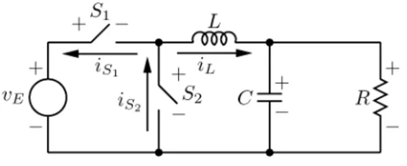
Example III.1: Consider the circuit shown in Fig. 1. This
cir-cuit can be obtained from the classical Buck converter topology by replacing the diode with an ideal switch . Suppose that the resistor, the capacitor, and the inductor are all linear ele-ments. A possible LSS description (see Example VI.7) can be obtained as follows:
(3a)
(3b) (3c)
where , and
. As the circuit contains two switches, there are four possible switch configurations, shown in the equation at the bottom of the next page.
Fig. 1. Buck converter.
A. Dynamics in a Switch Configuration
Given a fixed switch configuration , the
dynamics of the LSS (1) is given by the differential-algebraic equations (DAEs)
(4a) (4b) (4c) (4d) where the complement of is denoted by , that is
. Here, we use the notation where to denote the elements of that are
in-dexed by the set and where ,
to denote the submatrix obtained from
by taking the rows indexed by and the columns indexed by .
Also, we denote with by and
with by .
B. Solution Concept
In what follows we define what we mean by a “solution” to the (4). To avoid certain technicalities that would blur the main message of the paper, we deal only with Bohl-type inputs (i.e., polynomials, sinusoids, exponentials, and finite sums and prod-ucts of these) in the sequel.
Definition III.2: We say that:
• a continuously differentiable function is a solution with respect to the switch configuration for the initial state and the input if the DAEs (4) are satisfied for all
and ;
• an input is admissible with respect to the switch config-uration if the DAEs (4) admit a solution at least for an initial state ;
• an initial state is consistent with respect to the switch configuration and the admissible input if the DAEs (4) admit a solution.
Fig. 2. Two capacitors.
Two examples that illustrate the concepts of admissibility and consistency are in order.
Example III.3: Consider the Buck converter of Example III.1
and suppose that both switches are closed, i.e., the switch con-figuration is given by . Now and the dynamics are governed by the following DAEs:
(5a) (5b) Equation (5b) imposes a constraint on the input, namely . As such the only admissible input with respect to this switch configuration is the zero input.
Example III.4: Consider the circuit depicted in Fig. 2. It can
be put in the LSS form as follows:
(6a) (6a) (6c) Suppose that the switch configuration , i.e., the switch is closed. For this configuration, the DAEs (4) are given by
(7a) (7b) The algebraic equation (7b) implies that an initial state is consis-tent if and only if . Note that given a consistent initial state the DAEs (7) admit the unique
so-lution for all .
Our first aim is to give a complete characterization of admis-sible inputs and consistent initial states for a given circuit and
switch configuration. For this, we will work in the framework of LSS (1) and exploit the passivity of the underlying linear system. Next, we summarize the notion of passivity.
IV. PASSIVITY
This section is devoted to the notions of passivity and posi-tive realness. We quickly review the definition of passivity and its relation to positive realness as well as the implications of pas-sivity that will be used throughout the paper.
Having roots in circuit theory, passivity is a concept that has always played a central role in systems theory. Roughly speaking, a system is passive if the increase in the stored energy does not exceed the supplied energy.
Definition IV.1 [28]: A linear system given by
(8a) (8b) is called passive if there exists a nonnegative-valued function such that for all and all trajectories of the system (8) the following inequality holds:
(9)
If it exists the function is called a storage function.
An intimately related concept to passivity is positive realness.
Definition IV.2: A rational matrix is pos-itive real if
• is analytic in ;
• for all .
Here denotes the open right halfplane in .
The relation between passivity and positive realness is known as the Kalman–Yakubovich–Popov lemma. The fol-lowing proposition states this relation together with some other well-known implications of passivity.
Proposition IV.3 [28]: Consider the following statements.
1) The system is passive.
2) The linear matrix inequalities (LMIs)
(10) have a solution .
3) The function defines a storage
func-tion.
4) The transfer matrix is positive real.
5) The triple is minimal. 6) The pair is observable. 7) The matrix is positive definite.
The following implications hold.
A) 1 2 3.
B) 2 4.
C) 4 and 5 2. D) 2 and 6 7.
V. A COMPLETECHARACTERIZATION OFADMISSIBLEINPUTS ANDCONSISTENTINITIALSTATES
The purpose of this section is to give a complete characteri-zation of admissible inputs and consistent states. The two main
ingredients are the LSS framework and the notion of passivity that are discussed in the previous sections.
Note that the Laplace transform is a bijection between Bohl functions and strictly proper rational functions. By employing this correspondence, one can treat the DAEs (4) in the Laplace domain. This formulation, together with the passivity property, leads to the following complete characterization of admissible inputs and consistent initial states.
Theorem V.1: Consider the LSS (1). Suppose that the system
is passive with a positive definite storage func-tion. Then the following statements hold.
1) An input is admissible with respect to the switch config-uration if and only if
(11) 2) An initial state is consistent with respect to the switch configuration and the admissible Bohl-type input if and only if
(12)
Remark V.2: Theorem V.1 generalizes the results of [21],
[27] in two respects: it allows presence of inputs and it does neither assume minimality of the triple nor injectivity of . Note that the latter assumption does not hold in many examples that appear in practice, see, e.g., Examples III.1 and VII.5.
Remark V.3: Consider the network of Example III.1 with the
switch configuration . Note that , ,
and . As such, the condition (11) states that the only admissible input for this configuration is .
Remark V.4: Consider the network in Example III.4. Since
the corresponding matrix is zero, all inputs are admissible for all configurations. Consider the switch configuration
. Note that , , and . By
applying condition (12), we see that the initial state is consistent
if and only if . Note that if (i.e., the
switch is open), condition (12) drops out and all initial states are consistent.
VI. INCONSISTENTINITIALSTATES
Having established complete characterization of consistent initial states, we focus on inconsistent initial states in this sec-tion. First, we begin with the well-known example of two ca-pacitors. This is followed by the introduction of the so-called energy-based jump rule which is one of the main contributions of the paper. Finally, we show the equivalence of this new rule to those of the Laplace transform based method and the charge/flux conservation based method.
Consider the circuit given in Example III.4. When the switch is closed, the initial state is consistent only
if . Otherwise one should expect an
in-stantaneous jump in the state so that . The standard ways of computing this jump is to employ charge/flux conservation principle or Laplace transform method.
In this very simple example, the former method yields (13a) (13b)
Hence, we get
(13c) For the Laplace transform method, one has to solve the alge-braic relations obtained by taking the Laplace transform of (6). This would result in
(14) and hence (13c) by the initial value theorem of Laplace trans-form. Although the Laplace transform method yields the same results it may not be preferable for complex networks as it ne-cessitates symbolic manipulations.
In what follows, we propose a novel approach for the com-putation of the state jump. This new approach is based on the stored energy of the system and gives an explicit formula for the state after the jump in terms of the LSS form (1) and the chosen switch configuration. Its main advantages are to reduce the required computational power significantly and to provide further insight to state discontinuities caused by switching.
Later, we will show that the new jump rule is equivalent to charge/flux conservation rule, as well as the Laplace transform method, for linear passive electrical networks.
A. Energy-Based Jump Rule
Inspired by the jump rules that are employed in the context of mechanical systems with unilateral constraints (see [29]–[31]) and of electrical networks with switching elements (see [21], [27], [32]), we introduce an energy-based jump rule in what follows.
Theorem VI.1: Consider the LSS (1). Suppose that is passive with a positive definite storage function. Let be an initial state,
be a switch configuration, and be an admissible Bohl-type input with respect to the switch configuration . Consider the minimization problem
(15a) (15b) Then, the following statements hold.
1) For any positive definite solution of the LMIs (10), the quadratic program (15) has a unique solution.
2) The unique solution of (15), , can be explicitly given by
(16) where is a matrix with appropriate dimensions such that . Moreover, is the solution of (15) if and only if
(17a) (17b) 3) If and are two positive definite solutions of the
LMIs (10), then .
We define the unique value obtained by the above minimiza-tion problem as the reinitialized state for the energy-based jump rule and denote it by . Note that if is a consistent ini-tial state with respect to an admissible Bohl-type input , i.e.,
, then ,
and hence .
Remark VI.2: One of the advantages of calculating the
reini-tialized state using the energy-based jump rule via (16) is its computational ease. This formula gives the reinitialized state in terms of the parameters of the system description of the LSS from (1) and the stored energy defined by the matrix . The computation based on (16) requires two ingredients: the ma-trices and . The rows of the matrix form a basis for the null-space of the matrix . As such, one can employ stan-dard numerical linear algebra routines, for instance MATLAB’s nullcommand. Computation of is quite straightforward by efficient LMI techniques (see, e.g., [33]), for instance, via the LMI Toolbox of MATLAB. Moreover, if the state variables are taken as voltages across capacitors and currents through induc-tors then the matrix can be directly obtained from the ca-pacitances and inductors as explained in detail in Remark VI.6. Once and are given, the explicit formula (16) requires only matrix inversion and multiplication.
B. Reinitialization via Laplace Transform Method
Another common method to resolve the jump issue is to use the Laplace transform. For a given switch configuration , one can take the Laplace transform of (4). This yields
(18a) (18b)
(18c)
(18d) where is the Laplace transform of the corresponding variable,
whereas and
are obtained from (1). For an initial state and input , one looks for a solution of (18). The following theorem provides conditions of solvability for these equations in case the underlying linear system is passive.
Theorem VI.3: Consider the LSS (1). Suppose that is passive with a positive definite storage
function. Let be an initial state, be
a switch configuration, and be an admissible Bohl-type input with respect to the switch configuration . Then, the following statements hold.
1) The equations in (18) admit a solution
where the pair is proper and is strictly proper.
2) If with , 2 are two solutions,
then
(19b) (19c)
We define the unique value as the
reini-tialized state for the Laplace transform method.
Remark VI.4: In order to compute the reinitialized state with
Laplace transform method, one has to solve (18c) for . This requires symbolic manipulation which increases compu-tational burden heavily. In the literature, semisymbolic com-putation methods for solving (18c) have been introduced (see, e.g., [34]). These methods are based on interpolations on the unit circle and reduce the heavy computational burden of purely symbolic computations. Since the explicit formula (16) requires only matrix inversion and multiplication, the proposed method has a clear computational advantage over the Laplace transform method regardless of whether purely symbolic or semisymbolic techniques are employed. However, the explicit formula (16) is valid only for passive networks whereas the Laplace transform method is applicable to more general networks.
C. Equivalence of Energy-Based Jump Rule and Laplace Transform Based Jump Rule
So far, we have introduced a jump rule based on energy min-imization and discussed the Laplace transform based jump rule. It turns out that the Laplace transform based and the energy-based jump rules are equivalent as stated in the following the-orem.
Theorem VI.5: Consider the LSS (1). Suppose that is passive with a positive definite storage
function. Let be an initial state, be
a switch configuration, and be an admissible Bohl-type input with respect to the switch configuration . Then
D. Charge/Flux Conservation Principle
Our next aim is to show that the energy-based jump rule and the principle of charge/flux conservation (for linear circuits con-taining resistors, capacitors, inductors, independent voltage/cur-rent sources, and ideal switches) yield the same reinitialized state.
In the general framework of LSS (1), the state variable does not necessarily consist of capacitor voltages and inductor cur-rents. As such, one cannot directly apply the charge/flux con-servation principle to a general LSS.
First, we begin with deriving a particular LSS form of an elec-trical network (consisting of resistors, capacitors, inductors, in-dependent voltage/current sources, and ideal switches) in such a way that the charge/flux conservation principle can be related to this LSS form.
1) Derivation of Circuit Equations: Consider a network
whose elements are resistors, inductors, capacitors, independent sources, and switches. Suppose that the graph2 associated to
the network is connected and that capacitors do not form a loop (with or without voltage sources) and inductors do not form a cut set (with or without current sources). This assumption is
2We refer to [35] and [36] for the fundamental concepts of circuit theory.
not restrictive since if such a loop is present, one can break the loop by putting a switch in series to a capacitor (in the loop) and choose the switch configuration such that this extra switch is closed. A dual approach can be taken for inductors.
In order to obtain circuit equations, we first extract the ideal switches to the ports. For the remaining circuit, we consider a
proper tree, i.e., a tree that contains all the voltage sources and
the capacitors in the network, but no inductors and no current sources. It is always possible to find a proper tree (if no loops of capacitors/voltage sources and no cut sets of inductors/cur-rent souces are present). The capacitors are included in the tree branches, while the inductors in the links. The resistors, sources, and switches are included either in the branches or in the links in order to complete the tree. We partition the links and branches into eight subsets, namely the resistive links, the inductive links, the independent current source links, the port links, the capac-itive branches, the resistive branches, the independent voltage source branches, and the port branches. Let be the number of the links and be the number of the branches. The Kirchhoff voltage law (KVL) applied to the fundamental loops and the Kirchhoff current law (KCL) to the fundamental cut sets are obtained as follows:
(20)
where , , , , , , , and are subvectors repre-senting, respectively, voltages for the resistive links, the induc-tive links, the independent current source links, the port links, the capacitive branches, the resistive branches, the independent voltage source branches and the port branches; , , , , , , , and are subvectors representing, respectively, currents for the resistive links, the inductive links, the indepen-dent current source links, the port links, the capacitive branches, the resistive branches, the independent voltage source branches, and the port branches.
For the resistors, capacitors, and inductors, the constitutive laws of are given by
(21) where , , , and are diagonal matrices with positive diagonal elements (or positive definite matrices to be more gen-eral) of appropriate sizes.
For the ideal switches, the constitutive laws are given by (22a) (22b)
where , , , and .
Let
be a partition of the matrix that conforms with the (20). Using the KVL/KCL (20) and constitutive laws of the el-ements (21), one can obtain the following LSS form for the network:
(24a) (24b) (24c) (24d)
for and , where and
are the number of switches belonging to the port branches and to the port links, respectively. Here, the matrices are reported in (24e)–(24j), shown in the equation at the bottom of the page.
Remark VI.6: Naturally, the linear system
given by (24a) and (24b) forms a passive system with the storage function
Indeed, this choice results in
(25)
(26) Note that is clearly positive definite.
Example VI.7: Consider the circuit depicted in Fig. 1. By
taking a tree consisting of the voltage source , the switch , and the capacitor ; and applying KVL, one arrives at the equations
This results in
where
Next, we formalize the charge/flux conservation principle with the help of the special LSS form obtained above.
2) Formulation of Charge/Flux Conservation Principle: The
principle of charge/flux conservation is applied to a network in order to obtain consistent initial conditions for the state variables (capacitance voltages and inductance currents). The principle of
(24e) (24f) (24g) (24h) (24i) (24j) (24k) (24l)
TABLE I
TRANSFERREDCHARGE/FLUXRELATIONS FORCIRCUITELEMENTS
charge conservation states that the total charge transferred into a junction or out of a junction at any time is zero. Dually, the principle of flux conservation states that the flux summed over any closed loop is continuous. As such, KCL is valid in terms of the transferred charges for a node and KVL is valid in terms of the transferred fluxes for a loop with the definitions of trans-ferred charges/fluxes for different elements shown in Table I. In this table, denotes the corresponding value before disconti-nuity and after discontinuity.
For the principle of charge conservation, these definitions, together with (20), yield
(27a) and
(27b)
where , , , and , respectively, correspond to the charges transferred to the capacitors, voltage sources, port branches, and port links.
From (20), the KVL after the discontinuity is given by
(27c)
Analogously, it is possible to derive a set of equations for the principle of flux conservation
(27d) and
(27e)
where , , , and , respectively, correspond to the fluxes transferred to the inductors, current sources, port branches, and port links.
From (20), the KCL after the discontinuity is given by
(27f)
Finally, the constitutive laws of the switches have to be considered
(27g)
(27h)
where , , , and .
Remark VI.8: The existing methods based on the charge/flux
conservation principle (see, e.g., [8], [10], [19]) require the cir-cuit equations for the given switch configuration as input. When one wants to analyze another switch configuration, the corre-sponding governing equations should be derived for the new configuration. The LSS framework makes it possible to apply the charge/flux conservation principle to any switch configura-tion without deriving the circuit equaconfigura-tions for each topology. To our knowledge, the formalization of the charge/flux conserva-tion principle for an arbitrary switch configuraconserva-tion had not been studied in the literature before.
With all above preparations, we are ready to show the equiv-alence of the charge/flux conservation principle to the energy-based jump rule in what follows.
E. Equivalence of Charge/Flux Conservation Principle and Energy-Based Jump Rule
Principle of charge/flux conservation says that and , satisfying the relations in (27) for a given switch configuration, , , , and , should be taken as the reinitialized state for the network. Naturally, one should ask if there exists a solution and that satisfy those relations. If such a solution exists, the next natural question is to ask whether it is unique. To our knowledge, these questions have not been formally answered in the literature.
In what follows, we will show that any solution and for the relations in (27) coincides with the one obtained from energy-based jump rule. Hence, this solution is the unique so-lution.
Theorem VI.9: Consider the . For any given switch configuration, , , , and , the reinitialized state obtained by charge/flux conservation principle (27) coincides with the reinitialized state obtained by energy-based jump rule. As such charge/flux conservation principle (27) always yields a unique solution.
Remark VI.10: Together with the general formulation of
charge/flux conservation principle based on the LSS frame-work, above theorem indicates that the energy-based jump rule has no computational advantage over that of charge/flux conser-vation principle. However, the existing methods (see, e.g., [8], [10], [19]) based on charge/flux conservation principle require the derivation of corresponding circuit equations for the given configuration. Thanks to the LSS framework, the energy-based jump rule is given as an explicit formula which works for any switch topology without deriving governing equations of each topology separately. In this sense, the energy-based jump rule has considerable computational advantage over the existing methods based on charge/flux conservation principle.
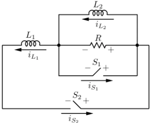
Fig. 3. Switched network of Example VII.3.
VII. EXAMPLES
In this section, we illustrate the computational simplicity of the new method on some examples considered in the literature within the context of switched electrical networks. The first one is the ubiquitous two-capacitor example.
Example VII.1: Consider the circuit depicted in Fig. 2. An
LSS form for this circuit was given in (6). Suppose that the switch configuration is given by , i.e., the switch is closed. Since , one can take in Theorem VI.1. Note that can be taken as a diagonal matrix with the diagonal elements and . Then, it follows from Theorem VI.1 that
(28)
Example VII.2: Consider the circuit depicted in Fig. 1. An
LSS form for this circuit was given in (3). Take . Since , one can take in Theorem VI.1. Note that can be taken as a diagonal matrix with the diagonal elements and . Then, it follows from Theorem VI.1 that
Example VII.3: Consider the circuit depicted in Fig. 3 that
was investigated in [10]. It can be expressed in the LSS form as follows:
Take . Since , one can take in
Theorem VI.1. Note that can be taken as a diagonal matrix with the diagonal elements and . Then, it follows from Theorem VI.1 that
Fig. 4. Switched network of Example VII.4.
Fig. 5. Switched network of Example VII.5.
Example VII.4: Consider the circuit depicted in Fig. 4 that
was investigated in [11]. It can be expressed in the LSS form as follows:
Take . Since , one can take . Note that
can be taken as a diagonal matrix with the diagonal elements and . Then, we get
Example VII.5: Consider the circuit depicted in Fig. 5 that was investigated in [1, Sec. IV-C]. It can be expressed in the LSS form as follows:
Take . Since , one can take in Theorem
VI.1. Note that can be taken as a diagonal matrix with the diagonal elements and . Then, it follows from Theorem
VI.1 that
VIII. CONCLUSIONS
A single compact framework called linear switched systems was employed for linear networks with ideal switches; this framework, which is valid for any switch configuration unifies and simplifies the analysis of such circuits. Within this frame-work, a complete characterization of admissible inputs and consistent states was presented. Under the passivity assumption for general systems, a new state reinitialization method based on energy minimization was developed. The advantages of the method, besides providing a clear insight to state discontinu-ities, are threefold.
• It is independent of any network topology and nature (ap-plicable to any linear switch system).
• It is computationally simpler over the existing methods which need to reanalyze the circuit each time a new switch configuration is adopted.
• More importantly, it provides once more a proof that nature settles itself by consuming the minimum amount of energy. This new method was shown to yield the same reinitialized state as:
• the one provided by using the Laplace transform tech-niques applied to linear switch systems (without any dis-tribution theory or any Dirac delta functional);
• the charge/flux conservation principle based state reinitial-ization rules (by providing a rigorous derivation for elec-trical circuits).
Two main directions arise as possibilities for further research. Extensions of the presented results for networks containing other types of switching elements such as ideal diodes and thyristors forms one of these directions; the other direction is to investigate the energy-based reinitialization rule for active and/or nonlinear circuits.
APPENDIX
PROOFS
For the proofs, we need two auxiliary results. The first one is concerned with the consequences of passivity.
Lemma A.1 [32, Lemma 2.5]: Suppose that the system
is passive. Let be any solution to LMIs (10)
and let . Then, the following
statements hold.
i) is positive semidefinite.
ii) .
iii) .
iv) for all complex numbers .
v) for all real positive
numbers that are not eigenvalues of .
The second auxiliary result provides conditions for the solv-ability of rational equations under a passivity assumption.
Theorem A.2: Consider the rational equation
(29) where the matrices , , , , , are of appropriate sizes, is a strictly proper rational, and a rational function. Suppose that the linear system is passive with a positive definite storage function. Then, the following statements hold.
1) The following statements are equivalent.
a) The relation is satisfied for all .
b) Equation (29) admits a solution for a given and .
c) Equation (29) admits a proper solution for a given and .
Moreover, if and are two solutions to (29), then .
2) The following statements are equivalent.
a) The relation is satisfied for all
and .
b) Equation (29) admits a strictly proper solution for a given and .
Proof: 1a 1b: Let and . It follows from [37, Th. 4.1] that (29) admits a solution if and only if
(30) admits a solution for all sufficiently large real numbers . Since
for all , for all real
numbers . Therefore, it would suffice to prove that
(31) for all sufficiently large real numbers . To see this, let be a positive real number greater than all real eigenvalues of . Also let . Due to passivity, is positive semidefinite.
This means that . By using Lemma A.1
v) and iv), we get . This means . From
Lemma A.1 v) and iii), we already have . Then, we get
(32) To see the reverse inclusion, let . Thus,
and . From Lemma A.1 i), we know that is positive semidefinite. This allows us to say that
. By invoking Lemma A.1 iii), iv), and v), we get . This means that . Therefore,
(33) Then, (31) follows from (32) and (33).
1b 1c: Let be a solution to (29). Suppose that
where . If
then is proper. Suppose that . Note that (29) implies that
(34) (35)
since these are the coefficients of and of the right hand side. By left-multiplying the latter by and using Lemma A.1 ii) and iv), one gets
(36)
This means that is also a solution of (29).
Clearly, one can find a proper solution by employing the above argument repeatedly.
1c 1a: Let be a proper solution to (29). Note that
lies in .
the rest of 1: It follows from (29) that
(37) From Proposition IV.3.4 and Lemma A.1.i), we get that
(38) for all sufficiently large positive real numbers . Since is rational, we can further conclude that
(39)
2a 2b: From the first part of the theorem, we know that (29)
admits a proper solution, say . Let
where . From (29), we get
(40) (41) By left-multiplying the latter by , using Lemma A.1 ii) and
iv), and the fact that , one gets
(42) Consequently, is a strictly proper solution to (29).
2b 2a: The relation readily follows from the first part of the theorem. Let be a strictly proper solution
with where . It
follows from (29) that
(43)
Hence, .
A. Proof of Theorem V.1
1) Necessity readily follows from (4c). For sufficiency, let
be such that . Take ,
, , , , and
. Since is passive with some positive
storage function, so is with the same storage function. By applying Theorem A.2, we get the desired solution for the initial state and the input .
2) Similar to the previous case, necessity immediately follows from (4c) and sufficiency can be proven by applying the very same argument.
B. Proof of Theorem VI.1
1) Let be a matrix of appropriate dimensions such that . Then, the constrained minimization problem (15) can be rewritten as
Let be the Lagrangian associated to this problem, i.e.,
By differentiating with respect to the unknown and the Lagrange multiplier and equating these derivatives to zero, one gets
(44a) (44b) These conditions are known as Karush–Kuhn–Tucker con-ditions (see, e.g., [38]) and they are known to be necessary conditions for optimality. When the cost function is convex and the constraint set closed, they are also known to be suf-ficient conditions for optimality (see, e.g., [38]). Note that the cost function of (15) is (even strictly) convex as is positive definite and the constraint set is closed as it is given by linear equations. Hence, we can conclude that the above Karush–Kuhn–Tucker conditions are necessary and suffi-cient for being a solution of (15). By solving from the first condition, one obtains
(45) It follows from elementary linear algebra that . This means that this linear equation has a solution if and only if . To see that this condition holds, note that
since is admissible. As by definition, one gets
Hence (45) has always a solution. To conclude the proof, it remains to show the uniqueness of this solution. Let and be two solutions of the Karush–Kuhn–Tucker con-ditions. It follows from (45) that
Since is positive definite, is
pos-itive semidefinite and hence . Therefore, one gets
from the first of the Karush–Kuhn–Tucker conditions. Since is positive definite, this yields .
2) The expression (16) readily follows from (44a) and (45). To prove that (17) holds, observer first that (17b) immediately follows. For (17a), note that
due to (44a). Since and is positive
semidefinite [Lemma A.1 i)], one gets . Hence, one has
It follows from Lemma A.1 ii) that and hence
3) Let and are two positive definite solutions of the LMIs (10). Also let and be the corresponding solutions of (15). It follows from (17)
Hence, we get
Let be any positive definite solution to the LMIs (10). The former relation, together with Lemma A.1 iii), results in
(46) whereas the latter yields
(47) where
. Since is positive semidefinite due to passivity, we
have where denotes the
orthog-onal subspace. Then, basic linear algebra implies that (48) Thus, (46) and (47) imply that
(49) As is positive definite, we finally get
(50)
C. Proof of Theorem VI.3
1) Note that (18) admits a solution if and only if (18c) admits a solution. Then, the claim follows from Theorem A.2 by choosing , , , , , and as in the proof of Theorem V.1.
2) Note that (19b) readily follows from Theorem A.2.1. The relations (19a) and (19c) follow from (18a), (18d), (19b), and Lemma A.1 v).
D. Proof of Theorem VI.5
We know from Theorem VI.3 that (18) admits a solution
where the pair is proper and
is strictly proper. Let have the expansion
(51) From (18a) and (18c), we get
(52a) (52b) (52c) Equivalently (53a) (53b) Consequently, the claim follows from Theorem VI.1.2.
E. Proof of Theorem VI.9
For notational simplicity, we give a proof of the case for which all switches on the links are closed and on the branches are open. The general case follows in the same lines.
Since all switches on the links are closed and on the branches are open, we get
(54a) (54b) In view of Theorem VI.1, we need to show that
(55) (56) To do so, we first claim that
(57)
To see this, note that
(58) (59) Thus, we also get
As a result,
(61)
Since the reverse inclusion readily follows from the structure of , (57) holds.
To establish (55), first note that we get
(62) from the second and fourth row blocks of (27b), the first and the fourth row blocks of (27e), and (57). Then, we have
(63) Since due to the first row block of (27b) and due to the second row block of (27c), we get (64) In view of (62), this implies (55).
To establish (56), note first that
(65) due to the semidefiniteness of and (57). Since
(66) due to the structure of , it is enough to show that the last sum-mand on the left-hand side lies in . This, however, follows from (54) and the last row blocks of (27c) and (27f).
REFERENCES
[1] S. Seshu and N. Balabanian, Linear Network Analysis. New York: Wiley, 1964.
[2] A. Dervisoglu, “State equations and initial values in active RLC net-works,” IEEE Trans. Circuit Theory, vol. CT-18, no. 5, pp. 544–547, 1971.
[3] M. Liou, “Exact analysis of linear circuits containing periodically op-erated switches with applications,” IEEE Trans. Circuit Theory, vol. 19, no. CT-2, pp. 146–154, 1972.
[4] A. Opal and J. Vlach, “Consistent initial conditions of linear switched networks,” IEEE Trans. Circuits Syst., vol. 37, no. 3, pp. 364–372, Mar. 1990.
[5] A. Opal, “The transition matrix for linear circuits,” IEEE Trans. Comput.-Aided Design Integr. Circuits Syst., vol. 16, no. 5, pp. 427–436, May 1997.
[6] Q. Li and F. Yuan, “Time-domain response and sensitivity of peri-odically switched nonlinear circuits,” IEEE Trans. Circuits Syst. I, Fundam. Theory Appl., vol. 50, no. 11, pp. 1436–1446, Nov. 2003. [7] Z. Zuhao, “ZZ model method for initial condition analysis of dynamics
networks,” IEEE Trans. Circuits Syst., vol. 38, no. 8, pp. 937–941, Aug. 1991.
[8] A. Massarini, U. Reggiani, and M. K. Kazimierczuk, “Analysis of net-works with ideal switches by state equations,” IEEE Trans. Circuits Syst. I, Fundam. Theory Appl., vol. 44, no. 8, pp. 692–697, Aug. 1997.
[9] B. De Kelper, L. A. Dessaint, K. Al-Haddad, and H. Nakra, “A compre-hensive approach to fixed-step simulation of switched circuits,” IEEE Trans. Power Electron., vol. 17, no. 2, pp. 216–224, Mar. 2002. [10] Y. Murakami, “A method for the formulation and solution of circuits
composed of switches and linear RLC elements,” IEEE Trans. Circuits Syst., vol. 34, no. 5, pp. 496–509, May 1987.
[11] J. Tolsa and M. Salichs, “Analysis of linear-networks with inconsistent initial conditions,” IEEE Trans. Circuits Syst. I, Fundam. Theory Appl., vol. 40, no. 12, pp. 885–894, Dec. 1993.
[12] A. Opal and J. Vlach, “Consistent initial conditions of nonlinear net-works with switches,” IEEE Trans. Circuits Syst., vol. 38, no. 7, pp. 698–710, Jul. 1991.
[13] J. Vlach, J. M. Wojciechowski, and A. Opal, “Analysis of nonlinear net-works with inconsistent initial conditions,” IEEE Trans. Circuits Syst. I, Fundam. Theory Appl., vol. 42, no. 4, pp. 195–200, Apr. 1995. [14] A. Opal, “Sampled data simulation of linear and nonlinear circuits,”
IEEE Trans. Comput.-Aided Design Integr. Circuits Syst., vol. 15, no. 3, pp. 295–307, Mar. 1996.
[15] F. Del Aguila Lopez, P. Schonwilder, J. Dalmau, and R. Mas, “A dis-crete-time technique for the steady state analysis of nonlinear switched circuits with inconsistent initial conditions,” in IEEE Int. Symp. Cir-cuits Syst., 2001, vol. 3, pp. 357–360.
[16] I. C. Goknar, “Conservation of energy at initial time for passive RLCM network,” IEEE Trans. Circuit Theory, vol. CT-19, no. 4, pp. 365–367, Jul. 1972.
[17] P. Mayer, J. Jeffries, and G. Paulik, “The two-capacitor problem recon-sidered,” IEEE Trans. Educ., vol. 36, no. 3, pp. 307–309, Aug. 1993. [18] A. M. Sommariva, “Solving the two capacitor paradox through a new
asymptotic approach,” IEE Proc. Circuits Devices Syst., vol. 150, no. 3, pp. 227–231, 2003.
[19] D. G. Bedrosian and J. Vlach, “Time-domain analysis of networks with internally controlled switches,” IEEE Trans. Circuits Syst. I, Fundam. Theory Appl., vol. 39, no. 3, pp. 199–212, Mar. 1992.
[20] M. K. Camlibel, W. P. M. H. Heemels, and J. M. Schumacher, “On the dynamic analysis of piecewise-linear networks,” IEEE Trans. Circuits Syst. I, Fundam. Theory Appl., vol. 49, no. 3, pp. 315–327, Mar. 2002. [21] M. K. Camlibel, W. P. M. H. Heemels, A. J. van der Schaft, and J. M. Schumacher, “Switched networks and complementarity,” IEEE Trans. Circuits Syst. I, Fundam. Theory Appl., vol. 50, no. 8, pp. 1036–1046, Aug. 2003.
[22] F. Vasca, L. Iannelli, M. K. Camlibel, and R. Frasca, “A new per-spective for modeling power electronics converters: Complementarity framework,” IEEE Trans. Power Electron., vol. 24, no. 2, pp. 465–468, Feb. 2009.
[23] S.-C. Tan, S. Bronstein, M. Nur, Y. Lai, A. Ioinovici, and C. Tse, “Vari-able structure modeling and design of switched-capacitor converters,” IEEE Trans. Circuits Syst. I, Reg. Papers, vol. 56, no. 9, pp. 2132–2142, Sep. 2009.
[24] J. Ruiz-Amaya, M. Delgado-Restituto, and A. Rodriguez-Vazquez, “Accurate settling-time modeling and design procedures for two-stage miller-compensated amplifiers for switched-capacitor circuits,” IEEE Trans. Circuits Syst. I, Reg. Papers, vol. 56, no. 6, pp. 1077–1087, Jun. 2009.
[25] Y. Wang, M. Yang, H. Wang, and Z. Guan, “Robust stabilization of complex switched networks with parametric uncertainties and delays via impulsive control,” IEEE Trans. Circuits Syst. I, Reg. Papers, vol. 56, no. 6, pp. 2100–2108, Jun. 2009.
[26] F. del-Águila López, P. Palà-Schönwälder, P. Molina-Gaudó, and A. Mediano-Heredia, “A discrete-time technique for the steady-state anal-ysis of nonlinear class-E amplifiers,” IEEE Trans. Circuits Syst. I, Reg. Papers, vol. 54, no. 6, pp. 1358–1366, Jun. 2007.
[27] K. M. Gerritsen, A. J. van der Schaft, and W. P. M. H. Heemels, “On switched Hamiltonian systems,” presented at the 15th Int. Symp. Math. Theory Netw. Syst., South Bend, IN, 2002.
[28] J. C. Willems, “Dissipative dynamical systems part I: General theory,” Arch. Ration. Mech. Anal., vol. 45, no. 5, pp. 321–351, 1972. [29] J. J. Moreau, “Quadratic programming in mechanics: Dynamics of
one-sided constraints,” SIAM J. Control, vol. 4, pp. 153–158, 1966. [30] J. J. Moreau, “Liaisons unilaterales sans frottement et chocs
inelas-tiques,” C. R. Acad. Sci., Paris, Ser. II, vol. 296, no. 19, pp. 1473–1476, 1983.
[31] J. J. Moreau, “Unilateral contact and dry friction in finite freedom dynamics,” in Nonsmooth Mechanics and Applications, ser. CISM Courses and Lectures, J. Moreau and P. Panagiotopoulos, Eds. Wien, New York: Springer-Verlag, 1988, vol. 302, pp. 1–82.
[32] M. K. Camlibel, L. Iannelli, and F. Vasca, “Passivity and complemen-tarity,” Math. Program. A, 2008, submitted for publication.
[33] S. Boyd, L. E. Ghaoui, E. Feron, and V. Balakrishnan, Linear Ma-trix Inequalities in System and Control Theory, ser. Studies in Applied Mathematics 15. Philadelphia, PA: SIAM, 1994.
[34] J. Vlach and K. Singhal, Computer Methods for Circuit Analysis and Design. Dordrecht, The Netherlands: Kluwer Academic, 2003. [35] C. Desoer and E. Kuh, Basic Circuit Theory. New York:
McGraw-Hill, 1969.
[36] L. O. Chua, C. A. Desoer, and E. S. Kuh, Linear and Nonlinear Cir-cuits. New York: McGraw-Hill, 1987.
[37] W. P. M. H. Heemels, J. M. Schumacher, and S. Weiland, “The rational complementarity problem,” Linear Algebr. Its Appl., vol. 294, no. 1–3, pp. 93–135, 1999.
[38] O. Mangasarian, Nonlinear Programming. New York: McGraw-Hill, 1969.
Roberto Frasca (S’05-M’08) was born in
Ben-evento, Italy, in 1976. He received the M.S. degree in electronic engineering from the Università di Napoli Federico II, Naples, Italy, in 2003 and the Ph.D. degree in Automatic Control from the Università del Sannio, Benevento, Italy, in 2007.
In 2006 and 2007, he was a Visiting Scholar at the Department of Mechanical Engineering—Dynamics and Control, Eindhoven University of Technology, The Netherlands. Since 2008 he has been with AnsaldoBreda SpA, Naples, as a Propulsion System Designer. His research interests include modeling and design of power electronic converters, rapid control prototyping, and hardware in the loop simulations.
M. Kanat Camlibel was born in Istanbul, Turkey,
in 1970. He received the B.Sc. and M.Sc. degrees in control and computer engineering from the Istanbul Technical University, Istanbul, Turkey, in 1991 and 1994, respectively, and the Ph.D. degree from Tilburg University, Tilburg, The Netherlands, in 2001.
Between 2001 and 2007, he held postdoctoral posi-tions at the University of Groningen and Tilburg versity, Assistant Professor positions at Dogus Uni-versity, Istanbul, and Eindhoven University of Tech-nology. Since 2007, he has been an Assistant Pro-fessor at the University of Groningen, The Netherlands. He is a Subject Ed-itor for the International Journal of Robust and Nonlinear Control. His main research interests include the analysis and control of nonsmooth dynamical sys-tems, in particular piecewise linear and complementarity systems.
I. Cem Goknar (S’66–M’71–SM’77–F’05) was
born in Istanbul, Turkey. He received the B.Sc. and M.Sc. degrees from Istanbul Technical University, Turkey, and the Ph.D. degree from Michigan State University, East Lansing, in 1969.
He was a Visiting Professor at the University of California, Berkeley; University of Illinois at Ur-bana-Champaign; University of Waterloo, Canada; Technical University of Denmark at Lyngby; and a Full Professor at Istanbul Technical University from 1979 to 2000. Currently he is a Professor, and was the Electronics and Communications Engineering Department Founding Head, at Dogus University, Istanbul, Turkey.
Prof. Goknar is a Member of European Circuit Society Council, a Member of the IEEE Technical Committee on Nonlinear Circuits and Systems, and IEEE-CAS Chapter Chair, Turkey Section.
Luigi Iannelli (S’01-M’03) was born in Benevento,
Italy, in 1975. He received the Laurea degree in computer engineering from the University of Sannio, Benevento, in 1999, and the Ph.D. degree in infor-mation engineering from the University of Napoli Federico II, Naples, Italy, in 2003.
During 2002 and 2003 he visited, as a Guest Researcher, the Department of Signals, Sensors, and Systems, Royal Institute of Technology, Stockholm, Sweden. He was a Research Assistant at the Dipar-timento di Informatica e Sistemistica, University of Napoli Federico II, and since 2004, he has been an Assistant Professor of Automatic Control with the Department of Engineering, University of Sannio, Benevento. His current research interests include analysis and control of switched and nonsmooth systems, and automotive control and applications of control theory to power electronics.
Dr. Iannelli is a Member of the IEEE Control Systems Society, the IEEE Circuits and Systems Society, and the Society for Industrial and Applied Math-ematics.
Francesco Vasca (S’94-M’95) was born in Giugliano, Napoli, Italy, in 1967. He received the M.Sc. and Ph.D degrees in Electronic and Automatic Control Engineering from the University of Napoli Federico II, Italy, in 1991 and 1995, respectively.
Since 2000 he has been an Associate Professor of Automatic Control with the Department of En-gineering, University of Sannio, Benevento, Italy. His research interests include automotive control, modeling and control for power converters, and averaging of switched systems through dithering. Prof. Vasca is currently an Associate Editor for the IEEE TRANSACTIONS ON