Robust solutions to single and multi-period machine layout problems with interval flows

MULTI-PERIOD MACHINE LAYOUT PROBLEMS WITH

INTERVAL FLOWS

A THESIS

SUBMITTED TO THE DEPARTMENT OF INDUSTRIAL

ENGINEERING

AND THE INSTITUTE OF ENGINEERING AND SCIENCES

OF BILKENT UNIVERSITY

IN PARTIAL FULFILLMENT OF THE REQUIREMENTS

FOR THE DEGREE OF

MASTER OF SCIENCE

Özgür Atilla TÜFEKÇİ

September, 1997

INTERVAL FLOWS

A THESIS

SUBMITTED TO THE DEPARTMENT OF INDUSTRIAL ENGINEERING AND THE INSTITUTE OF ENGINEERING AND SCIENCES

OF BILKENT UNIVERSITY

IN PARTIAL FULFILLMENT OF THE REQUIREMENTS FOR THE DEGREE OF

MASTER OF SCIENCE

0 ^ ;r AVnla

Ozgiir Atilla Tiifekgi September, 1997

Assoc. Prof. Barbaros Tansel (Principal Advisor)

I certify that I have read this thesis and that in my opiiiion it is fully adequate, in scope and in quality, as a thesis for the degree of Master of Science.

Assoc. Prof. Osman Oğuz

I certify that I have read this thesis and that in my opinion it is fully adequate, in scope and in quality, as a thesis for the degree of Master of Science.

Assoc. Prof. Cemal Dinçer

Approved for the Institute of Engineering and Sciences:

Prof. Mehmet 'Qi

R O B U S T S O L U T IO N S T O SIN G L E A N D M U L T I-P E R IO D M A C H IN E L A Y O U T P R O B L E M S W IT H IN T E R V A L F L O W S

Özgür Atilla Tüfekçi M .S. in Industrial Engineering

Supervisor: Assoc. Prof. Barbaros Ç. Tansel September, 1997

Design clecisous are genevcUly given in the early stages when there is a great deal of inexactness in the data gathered. In this study, we consider the plant Uiyout problem witli inexactness in material flow quantities with the aim of designing robust layouts. Material flow quantities are assumed to lie in a priori specified intervals based, for example, on low ¿md high demands. The robustness criterion we use is to minimize the maximum I’egret. We extend our work to the multi-period case where a distinction is made l)etween reversible and irreversible layout decisions.

Key words: Plant Layout, robust optimization , inexact data. m

M A L Z E M E A K IŞ L A R IN IN A R A L IK D E Ğ E R L E R İY L E T A N IM L A N D IĞ I T E K V E Ç O K D Ö N E M M A K İN E Y E R L E Ş İM

P R O B L E M L E R İN E D A Y A N IK L I Ç Ö Z Ü M L E R

Özgür Atilla Tüfekçi

Endüstri Mühendisliği Bcilümü Yüksek Lisans Tez Yöneticisi: Doç. Dr. Barbaros Ç. Tansel

Eylül, 1997

Makine yerleijirn problemlerinde tasarım kararları, genellikle eldeki verinin yetersiz olduğu ön safhalarda verilir. Bu çalışmada, dayanıklı çözümler üretmek amacıyla, malzeme akış miktarlarının belirsiz olduğu durumlarda makine yerleşim problemleri İncelenmektedir. Malzeme akış miktarlanmu, akışların en az ve en çok olduğu durumlara karşılık gelen alt ve üst değerleri arasında önceden bilinmeyen bir değer alacağı varsayılmıştır. Dayanıklılık ölçütü olarak en fazla kaybı enazlama seçilmiştir. Çalışmada geri dönülebilir ve dönülemez kararların birbirinden ayrıldığı çok dönem problemine de yerverilrniştir.

Anahtar sözcükler: Makine yerleşimi, dayanıklı eniyileme, belirsiz veri.

I would like to dediciite this tluisis to my motliei; Ay.'je Erdal and my grandmother Hatice Çelik Гог their love and sacrilicies.

I am very grateful to Barbaros Ç. Tansel for suggesting this interesting research topic, also for supervising me with patience and everlasting interest. His guidance and encouragement has been so precious for me all through rny griiduate studies.

I am also indebted to Dr. Cemal Dinçer and Dr. Osman Oğuz for showing keen interest to the subject matter and accepting to read and review this thesis. Their remarks and recommendations have been invaluable.

I wish to express my gratitude to my mother-in-law and father-in-law; Munise and Bekir Tüfekçi who have always supported with me with love. Also to Ozan whose existence is enough to bring joy to our lives. And to Hasan whose friendship is invaluable.

I would also like to thank to my friends Muhittin Hakan Demir, Feryal Erhun, Bahar Kara, Alev Kaya, Kemal Kılıç, Serkan Özkan, Muzaffer Tanyer who sincerely gave all the help they could.

I am not able to express my thanks to Tolga, instead I choose to thank God for him.

1 IN TR O D U CTIO N

1.1 Introdu ction... 1

1.2 Literature related to “inexact” d a t a ... 2

1.3 Plant Laj'out P r o b l e m ... 14

1.4 M otivation... 19

2 SINGLE PERIOD CASE 2.1 Problem Definition and Form u hit ion 22 22 2.2 Reform ukition...25

2.3 Exploiting the Layout S tru ctu re... 28

2.4 Computational W o r k ... 32 3 MULTI-PERIOD CASE 35 3.1 Problem S ta tem en t... ... 35 3.2 Problem Formulation ...37 3.3 Reformulation . . 38 vn

3.4 Com])ulational Work 40

4 CONCLUSION 45

A Modeling “Inexactness” 51

2.1 Two possible layouts for 2 x 4 ... 29

2.2 fl'lireci layouts for the 2x2 grid that are not distance invariant... 30

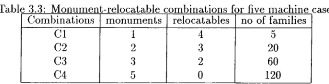
3.1 Iterations for all combinations of five m a c h in e ... 43

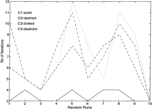
3.2 CPU Times for all combinations of live m a ch in e ... 44

3.3 Mciximum regrets lor all combinations of five machine ... 44

A .l Classification in terms of api)roaclies ... 52

A . 2 Classification in terms of data representation t y p e s ... 53

B . l Layout for five m a ch in e s... 55

B.2 Layout for six machines ...55

B.3 Layout for seven m a ch in e s... 55

B.4 Layout for eight m a c h in e s ... 56

B.5 Layout for nine m achines...56

2.1 Clcissificatiou of the Laj^out.s for the 3x3 Grid 30

2.2 Number of iterations for Algorithm I ... 32

2.3 CPU Times for Algorithm I ... 32

2.4 CPU Times for complete enumeration... 33

3.1 Number of iterations for Algorithm I I ... 41

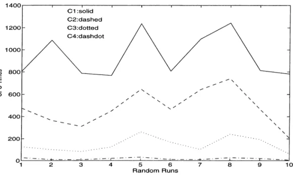
3.2 CPU Times for Algorithm I I ... 41 3.3 Monument-relocatable combinations for five machine case 42

IN T R O D U C T IO N

1.1

Introduction

In this thesis, the plant layout problem with imprecise data is investigated, with the aim of designing robust layouts. Plant layout problem is the problem of determining the relative locations of a given number of machines among the candidate locations. The objective is the minimization of the total material handling cost which is defined as the product of material flow and distances between the machines.

We consider plant layout problems with inexactness in material flow quantities. Layout decisions are generally given when neither the products nor the process plans are complete. Forecasting errors as well as fluctuations in demand are possible sources of uncertainty. As the planning horizon for the layout gets longer, even the product mix may change. Alternate and probabilistic routings make matters worse. As a result, the layout decisions are given with a great deal imprecision in material flow data. We express the data in terms of intervals specified by the lowest and highest values that the actual value can take. We assume that it is not possible to attribute probabilities to realizations of the material flow data.

In case of uncertainty, optimality with respect to an objective does not make much sense. The designer is usually interested in the robustness of the layout in that the layout should be good enough whatever data is realized. We will be using minmax regret criterion as our robustness measure.

With short planning horizons, the set of products is generally known with certainty. Estimation of production volumes then turns out to be the only source of inexactness. In this case we model the problem as a single period layout problem. On the other hand, longer horizons are subject to changes in the product mix and higher variability in production volumes. Dynamic layout decisions are needed in this kind of environments. We model this problem as a multi-period layout problem and differentiate the decisions as reversible and irreversible decisions. Robustness of the irreversible decisions is the major issue in the multi-period case.

In Chapter I, we introduce the literature on inexact data as well as the plant layout problem and state our motivation. In Chapter II, single period plant layout problem is defined and an algorithm is proposed to find a robust solution. Chapter III is a similar work for the multi-period problem. Then comes the conclusion in Chapter IV.

1.2

Literature related to “inexact” data

Mathematical programming models usually have the problem of noisy, erroneous or incomplete, i.e “inexact” data irrespective of the application domain. Cost of resources, demand for the products, returns of financial instruments are examples of data that are not known with certainty. In the literature many different ways of handling this imprecision are proposed. A brief survey of what has been done so far will be given in this section. Figure A .l shows the classification in terms of approaches whereas Figure A .2 is a classification in terms of data representation types.

Imprecision in data can be dealt with reactively or proactively. Reactive “post optimality” studies develop a deterministic model and use sensitivity analysis

to discover the effect of data perturbations on the model. Sensitivity analysis just measures the sensitivity of a solution to changes in the input data and offers local information near the assumed values. It provides no mechanism by which this sensitivity can be controlled. To do this a proactive approach is needed.

Proactive approaches can be classified with respect to the environments they are used in. There are two different kinds of environments: Risk and Uncertainty

situations. In risk situations, the link between decisions and outcomes is probabilistic. In uncertainty situations, it is imj^ossible to attribute probabilities to the possible outcomes of any decision.

In risk situations, a standard and simple approach is to replace the random parameters by their expectations and solve a deterministic model. This approach, called Expected Value Approach, has the disadvantage of ignoring much information contained in the probability distribution. Dantzig (1955), stimulated by discussions with A. Ferguson for the problem of allocation of carrier fleet to airline routes, extends LP models to include anticipated demand distributions in allocation problems. His studies can be considered as the beginning of stochastic modeling. His model is a classical two-stage stochastic program with simple recourse, where the allocation decisions are the first stage “design” decision variables and the resulting excess or shortage are the second stage “control” decision variables which depend on both the allocation plan and the realized demand. Design variables are the decision variables whose optimal values are not conditioned on the realization of uncertain parameters and they can not be adjusted once a specific realization of the data is observed whereas control decision variables are subject to adjustment once the uncertain parameters are observed. The optimal values of the control variables depend both on the realization and on the optimal values of design variables. For example, in the context of production processes, design variables determine the

size of the modules whereas the control variables denote the level of production in response to changes in the demand.

Dantzig (1955) establishes theorems on the convexity of expected objective functions and reduces the two stage stochastic problem into a standard LP. He also constructs similar theorems for m-stage case admitting that it has no significant computational value in this case. Wagner (1995) calls this type of stochastic models

Static Stochastic Planning Models .

Continuous distributions cause severe modeling problems when correlations exist for the random variables. Instead of using continuous distributions as Dantzig does, depending on the problem, one can choose to state risk in terms of scenarios where a scenario is defined as a particular realization of data. Modeling risk by a small number of versions of the problem which correspond to different scenarios is called Scenario Analysis . Suppose that Q = {1 ,2 ,3 ,..., S'} is a set of scenario indices. With each scenario index s € D, there is an associated set {d*, Bg, Cg, e«} of realizations for parameters related to control variables and control constraints and a probability pg. If one knew which scenario would occur, he could solve easily the corresponding deterministic problem obtained by replacing the parameter set with the values corresponding to that scenario. These solutions are called Individual Scenario Solutions and are of no help to the decision maker as it is not known which one will occur. Besides, there is no prescription as to how they can be aggregated to obtain a single policy that can be used by the decision maker. The major aim in scenario analysis is to study possible situations in terms of scenarios and to come up with a solution that can perform rather well under all scenarios. From now on all the models will be using scenario analysis unless otherwise stated.

Suppose that the deterministic optimization problem has the following structure:

Mill cx + dy s.t

Aa- = b B x + Cy = e

x , y > 0

X e R^\y e R^^

Then Static Stochastic Planning Model can be constructed as:

Min ^ dsysPs + cx

s = l

Ax = b...structural constraints

B s X + C 'sî/s = C s V s G 0 ...control constraints

x,ys ^ 0 Ws Ç. D

The particular block structure of this model is amenable to specially designed algorithms. Another approach that is often used with multi-period stochastic models is to use rolling horizon. After the model is run, the decisions for the first time period are implemented. Then the first stage risk parameters are realized, the model is adjusted and rerun. This approach is called Static Stochastic Planning Model W ith Rolling Horizon .

The model used in Static Stochastic Model and Rolling Horizon are the same, only the results are used differently. Advantage of rolling horizon approach is that it allows the decision maker to use the information gained as time passes although the design variables still remain fixed.

Escudero (1993), gives several stochastic multistage formulations of the production planning problem. By changing the control variables, many different recourse models are introduced for different cases of the problem. Full recourse

models are introduced where all variables are control variables. The main difference between the model given by Escudero and the models told above is that it is multistage. Escudero considers the “regret” associated with the solutions of the models introduced. Regret is defined as the difference between the cost of implemented solution and the individual optimal solution corresponding to the scenario which actually occurred and the regret distribution is defined as the distribution function of regret. The models are stated to produce solutions whose regret distribution most closely approximates the zero-regret distribution in the sense of minimal /1 distance between the inverse of regret distribution and the inverse of zero regret distribution.

D y n a m ic S to ch a stic P ro g ra m m in g (DSP) formulation allows design vari­ ables to react to information gained as scenarios unfold. It allows the decision maker the fullest response to changes in these parameters. The essential feature of DSP approach is the structuring of problems into stages, which are solved sequentially one stage at a time. Often the stages represent time periods in problem’s planning horizon. Associated with each stage of the optimization problem are the states of the process. The states reflect the information required to fully assess the consequences the current decision has upon future actions. The final general characteristic of DSP approach is the recursive optimization procedure which builds to a solution of the overall N-stage problem by first solving one stage problems until the overall optimum has been found. The basis of the recursive optimization is the “principle of optimality” : an optimal policy has the property that whatever the current state and decision, the remaining decisions must constitute an optimal policy with regard to the state resulting from current decision. Unfortunately DSP models are larger than the previous formulations and are difficult to solve.

Birge (1995), judges the value of stochastic models over deterministic models and states that stochastic models are more valuable as they have the capability to give solutions which hedge against multiple possible future outcomes when compared with deterministic LP models which tend toward extreme point solutions that rely on a limited set of activities. Birge gives a financial planning model to prove his

claim.

Mulvey, Vanderbei, and Zenios (1995), bring robustness criteria into stochastic models. They name their work as R o b u s t O p tim iz a tio n (R O ) and differentiate it from stochastic models although their models are usually stochastic in nature with some verifications from the above Static Stochastic Models to achieve robustness. Their approach integrates goal programming formulations with a scenario based description of the problem data in order to generate a series of solutions that are less sensitive to realizations of data from a scenario set. An RO model is:

M i n f { x , yi, ...,ys)

+

Wg(zi, Z2,

...,

z^)

Ax = b...structural constraints

BgX + Csys + Zg = Cs\/x G ...control constraints

XiVs

0

Robust Optimization (RO) is an extension of Static Stochastic Models with two major distinguishing features. First of all, feasibility is generally overemphasized in optimization problems. It may not be possible to get a feasible solution to a problem under all scenarios or the decision maker may be willing to sacrifice from feasibility for a better solution. RO allows for infeasibilies in the control constraints by introducing a set 2ti, ^2,..., of error vectors that measure infeasibility and add a component to the objective function that penalizes this infeasibility (infeasibility penalty function). The specific choice of penalty function gi^zi^z^·,..., Zg) is problem dependent, quadratic penalty function being applicable where both positive and negative violations are equally undesirable.

The second feature of RO that differentiates it from Static Stochastic Models is the introduction of higher moments in f{x ,y i,...,y g ). Expected value function ignores the risk attribute of the decision maker and the distribution of the objective values. Two popular alternative approaches are mean-variance models where the risk attribute is equated with variance and Von Neumann-Morgenstern expected

utility models. The primary advantage of expected utility model over mean variance approach is that asymmetries in the distribution are captured. The models told till RO optimize only the first moment of the objective function, ignoring the decision maker’s preferences toward risk. Hence they assume an active management style where the control variables are easily adjusted as the scenarios unfold. Large changes in the objective values may be observed among different scenarios, but their expected value will be optimal. The RO Model on the other hand minimizes higher moments, e.g. the variance, leading to a more passive management style. Since the objective value will not differ substantially among different scenarios, less adjustment is needed for control variables. Hence recourse decisions are implicitly restricted in RO. However, this will occur at a cost.

The RO Model has a multi criteria objective form with first term measuring optimality robustness second term penalizing infeasibility. The goal programming weight w is used to derive a spectrum of solutions. RO suffers from choice of this parameter w like other multi criteria programming models.

Dembo (1991), proposes another approach named Scenario Optimization.

First a solution is computed to the deterministic problem under all scenarios, then a coordinating or tracking model is solved to find a single policy.

A scenario problem is:

Vg = mmcsX Ax = b

BgX = Cg

X > 0

and a possible coordinating model is:

Ax = b X > Q

Instead of norm minimization which is a non differentiable function, other functions can be used.

This model is a special case of RO where only design variables and structural constraints are present. The main advantage of Dembo’s approach is that if all of the scenarios are known beforehand, they can be solved for once and for all. And at each period coordination problem with current best estimates of the scenario probabilities can be solved to determine the policy. The work required is multiple of that required for a scenario subproblem. Its major limitation is ignorance of adjustment to uncertain parameters by the use of control variables. But the model is easy to solve and has been successful in many applications.

Rockafellar and Wets (1991), propose solving a large deterministic equivalent of a multistage stochastic model obtained by scenario subproblems and nonanticipality constraints linking them. Their approach is called Scenario Aggregation (SA). Nonanticipality constraints ensure that if two different scenarios s and s’ are indistinguishable at time t on the basis of information available about them at time t, then the decision to be made should be the same at time t. They propose a “hedging” algorithm for solving the problem by a decomposition technique.

Some implementations of SA assume that the behavior of the random variables in all future stages can be predicted well and uses all the information on future events to hedge the decision made today. However in any cases estimates of the random parameters in future stages are extremely poor. For such situations, instead of using a multistage model like SA, a two stage model like SO can be used in a rolling horizon fashion.

probabilities to the possible outcomes of any decision. This can occur, for example, when the outcome of a decision depends on the decision of a competitor or on future external event which are not repeatable. In uncertainty situations, data can again be described in terms of scenarios, but this time there are no probabilities associated with each scenario representing its likelihood of occurrence. In addition to scenario analysis, interval analysis can also be used. In interval analysis, the interval, described by a lower and an upper bound, represents the range in which the true value lies. Another approach which captures interval analysis as a special case is to describe the data in a given convex set. Here the uncertain parameters are known to lie in some set described by exact functional relations. For example, the prices of electricity, coal, oil and gas are interrelated and a production planning problem can be modeled such that the objective value coefficients is a vector depending on energy prices and is constrained to lie in a set that reflects all realistic relations between these prices.

It is possible to convert an uncertainty problem into a risk problem, for example by subjective estimation of probabilities or by assigning equal probabilities to all possible outcomes of a decision (Laplace). When used appropriately this can be a valuable simplification. Assigning probabilities may make the decision maker feel comfortable, but one should be careful that the model reflects reality.

One possible uncertainty decision criterion is p e ssim istic d e cisio n crite rio n . The pessimistic decision criterion or what is sometimes called minimax or maximin criterion assures the decision maker that he will earn no less (or pay no more) than some specified amount. It is a very conservative approach in that it anticipates the worst that might well happen. This criterion is best suited for those situations where the probabilities can not be easily evaluated and the decision maker is conservative. Falk (1975), in his technical note, seeks maximin solution to linear programming programs whose objective function coefficients are known to lie in a given convex set. Falk represents optimality criteria that characterize the desired solution strengthening Solyster’s (1973-74a-74b) studies. His work is computationally implementable.

On the other hand, optimistic decision criterion or maximax minimax criterion, assures the decision maker that he will not miss the opportunity to achieve the greatest possible payoff or lowest possible cost. However, this decision making behavior usually involves the risk of a large loss. The approach is optimistic in that the best (maximum profit or minimum cost) is anticipated. The optimal strategy is then the best of the anticipated outcomes.

Another criterion, Hurwicz is a compromise between the pessimistic and optimistic criteria with weighting at the discretion of the decision maker.

One other possible criterion is minimax regret. Regret is used in the same meaning as defined previously. In this approach the first step is to compute regret associated with each combination of decision and possible outcome. The minimax criterion is then applied to the regret values to choose the decision with the least maximum regret. A decision using this criterion will be more conservative than maximax and less conservative than maximin, since it gives weight to missed opportunities.

Rosenhead et al (1972), proposes a Robustness-Stability approach. He distinguishes plans from decisions by defining a plan as a set of prospective decisions to be implemented at different future dates. At any point in the life of a plan, some decisions may be changed depending on what uncontrollable and unpredictable events occur. As these events unfold, more information becomes available and the unimplemented stages of the plan are reconsidered and modified. If the possibility of revision is not considered in earlier implemented decisions of a plan, there may no longer be adequate residual flexibility. Gupta and Rosenhead (1968), Rosenhead et al (1972) define robustness as a measure of the useful flexibility maintained by a decision for achieving near optimal states and consider it as a suitable criterion for sequential decision making under uncertainty. In mathematical notation; let

Any initial decision will restrict the attainable plans to a subset Si of S. Suppose some subset

S~

S

di

n{Si~)ln{S~).

V{sj) be the value (e.g cost ) of the plan Sj , then a modified robustness index is

n = T,sjQS- y ( s j) which is more suitable if variations of value within

S~

Rosenhead et al, defines one more decision criterion “ stability “in the following way: an initial decision (or decisions) is stable if the system modified by this decision has a long run performance which is satisfactory if no further stage of the plan is implemented. Both robustness and stability are criteria for the choice of initial decision from the decision set rather than the plan set.

The main assumption implicit in robustness analysis is that solutions which appear “good” in terms of the predicted values are more likely to be good under the conditions which are eventually realized. This assumption is very questionable. Robustness measured based on

S

Rosenblatt and Lee (1987) extend the robustness approach to layout problems. According to their approach robustness of a layout is an indicator of flexibility in handling demand changes and is measured by the number of times that the layout has a total material handling cost within a prespecified percentage of the optimal solution under different demand scenarios. So it is aimed to select a layout that has the highest frequency of being closest to the optimal solution even though it may not be optimal under any demand scenario. Being within a few percentage of optimal is perceived as satisfactory given the level of inaccuracy of the available data during the design phase.

with long planning horizons and for multi period layout designs. For multi-period dynamic layout designs they generate the sequence of robust layout which also satisfy the restriction that difficult to relocate processes should remain at the same positions in multi-period layouts. More information will be given about their work in the following sections.

As stated previously in interval analysis, uncertainty can also be described in terms of intervals. Ishibuchi and Tanaka (1990) convert linear programs with interval objective functions into multi objective problems with two objectives: optimization of the worst case and average case by use of order relations. The solution sets of the original problems with interval objective functions are defined as the pareto optimal solutions of the corresponding multi objective problems.

Demir (1994), Tansel and Demir (1996) deal with locational decisions where uncertainty is represented by intervals. “Weak” , “ Permanent” and “Unionwise permanent“ optimality criteria are defined on the basis of how much of the region of uncertainty a given solution optimally accounts for. The weak solution set consist of the locations which qualify as optimal for at least one realization of data. Permanent solutions are optimal for all data realizations, but they may not exist. Unionwise permanent solutions are collections of solutions at least one of which is optimal for every realization of data. Methods are given to construct small cardinality unionwise permanent solutions. A permanent solution, if it exists, is a robust solution with zero regret. In case it does not exist approximately permanent solutions are proposed which minimize the maximum violation in the necessary and sufficient conditions characterizing permanent solutions. Alternative approaches are implementing all solutions contained in a unionwise permanent solution or solving an auxiliary optimization problem which minimizes maximum regret by use of unionwise permanent solutions.

Inuiguchi and Sakawa (1995) deal with general linear programming problems with interval objective function coefficients. They develop parallel concepts with

Tansel and Demir. Permanent solutions are called “necessarily optimal” and weak solutions are called “possibly optimal” . They present a new treatment of interval objective function by introducing min max regret criterion as used in decision theory. Obviously necessarily optimal solution gives zero regret solution if it exists. They try to narrow the search space by using the properties of minimax regret solution and the relations with possibly and necessarily optimal solutions. They propose a method of solution by a relaxation procedure. We will be making use of their approach.

Inuiguchi and Sakawa’s solutions are more reliable than the solutions of the multi objective approach by Ishibuchi and Tanaka as the second one is reasonable only in the sati,sficing scheme. In addition to that, minimax regret formulation provides a solution which minimizes the worst difference of objective value. Since all the possibly optimal solutions are considered, the minimax regret formulation is closer to the formulation in optimizing scheme than the multi objective formulation.

1.3

Plant Layout Problem

Plant layout problem is often defined as the problem of determining the relative locations of a given number of machines among the candidate locations.

Generally two different approaches are used in stating the problem, one is qualitative and the other is quantitative. In the qualitative approach, the objective is the maximization of some measure of closeness ratings. ALDEP (Seehof and Evans 1967) and CORELAP (Lee and Moore 1967, Moore 1971) are computerized packages that work with this approach.

A typical quantitative objective is the minimization of the total material handling cost. In manufacturing systems, material handling cost is incurred for routing raw materials, parts, sub assemblies and other materials between different departments

(or machines). According to Tompkins and White (1984) “It had been estimated that between 20% and 50% of the total operating expenses within manufacturing are attributed to material handling. Effective facilities planning can reduce these costs by 10% to 30% and thus increase productivity.”

Material handling cost is defined as the product of material flow and distances between the machines. Material flow is calculated by using the production volumes and routes used in manufacturing these products. Flow data can be represented in terms of the actual amount of material moved or it may denote the number of trips performed by the material handling device between the machines. Distances between the machines can be expressed in terms of the actual distances or the travel time between the machines. Choices depend on the system that is investigated.

Heragu (1992) classifies the layout problem into three with respect to the physical environment: single-row layout problem, multi-row equal-area layout problem and multi-row unequal-area layout problem. In case of single-row layout, the machines are arranged linearly in one row. In multi-row, the machines are arranged linearly in two or more rows. The machines may be of equal or unequal area.

Based on the length of the planning horizon, Palekar et al (1992) classifies plant layout problems into two categories: Single Period Layout Problem (SPLP) and Dynamic Plant Layout Problem (DPLP). SPLP focuses on finding a layout for a single period while DPLP’s objective is to find a layout schedule for all periods in the planning horizon. The DPLP is further classified into two classes of problems: deterministic or stochastic according to the degree of risk with which the input information is known. Stochastic DPLP is the most complex as well as the most general of all cases. All other models may be viewed as special cases of the problem. Although Palekar skips the Single Period Stochastic case, there are also studies related to this model like Rosenblatt and Lee’s which we will mention.

problem : Q A P . The name is so given because the objective is a second degree quadratic function of the variables and the constraints are linear functions of the variables controlling the assignment of machines to locations. Given a set A = and nxn matrices W = (wij), D = {dki) and Ixn vector C = (cj), QAP can be stated as :

n n

M i U a e A Y , Y Wijda(i)a{j) + Y C ia{i)

¿=1

where A is the set of all permutations of N. In layout problems W is the flow matrix,

D is the distance matrix, and C is the vector denoting constant cost of assignment. The objective is to And an assignment of all facilities to all locations such that the total cost of the assignment is minimized. The linear terms can be elliminated from the problem by redefining the flow matrix.

QAPs is an NP-hard problem. This follows from the fact that TSP is a special QAP. On the other hand, any QAP can be solved by enumerating all of its n! feasible solutions. The best known algorithins (usually branch-and-bound type algorithms) have reportedly been successful mostly for instances of size n < 15. For n > 17, solution times of these algorithms tend to be prohibitive except for a few cases (Amcaoglu and Tansel 1997). The interested reader can refer to Pardalos, Rendl and Wolkowicz (1994) for a survey of the literature on QAP.

Other mixed-integer models, some of which are linearizations of the QAP, are also developed. In addition to that there are also some graph-theoretic models. Heragu (1992) presents a model with absolute values in the objective function and constraints for both single row and multi-row layouts problems.

Computerized packages are also available such as CRAFT (Buffa, Armour, Buffa 1964) and COFAD (Tompkins and Reed 1976). Three dimensional plant layout packages have also been developed, for example CRAFT3D (Cinar 1975) and SPACECRAFT (Johnson 1982) are these sort of packages.

Rosenblatt (1986) deals with the dynamic nature of the problem. A deterministic environment is assumed, where the number of orders and the quantities, arrival and due dates for different products are known for a given finite horizon. In this environment Rosenblatt determines what the layout should be in each period, or to what extent, if any changes in the layout should be made. He introduces rearrangement costs . Assuming T periods, the maximum number of combinations that need to be considered is (n!)^ which makes total enumeration prohibitive. Therefore a dynamic programming approach is suggested to solve the problem either in an optimal or heuristic manner when the number of departments is large.

Usually the environment is not deterministic for the layout designer. According to Kouvelis et al (1992) “The layout designer faces the difficult task of developing a system that is capable of handling a variety of products with variable demands at a reasonable cost. Alternate and probabilistic schedule and inventory constraints further complicate the task. To make matters worse, in some cases the required input data to layout decision process, e.g, the part production volumes, may be highly inaccurate. That might result from either the use of historical analogy approach in collecting the data or the usual forecast inaccuracies to large planning horizons used for layout design purposes.”

Rosenblatt’s deterministic approach is not suitable for the environment described above. Palekar et al (1992), deal with situations where changes in product mix, machine breakdowns, seasonal fluctuations and demand are only probabilistically known (Stochastic DPLP). Like Rosenblatt’s, this model also captures the relocation cost incurred whenever a layout is changed from one period to the next. The objective is minimizing the sum of expected material handling cost and relocation costs. An exact method and heuristics are suggested to solve the model.

Kouvelis and Kiran (1991) consider two cases in highly nondeterministic environments. In the first case, a layout cannot be changed in the planning horizon. During the layout design phase the product mix is uncertain, but once realized.

the product mix is expected to remain stable over the planning horizon. This is applicable in automated environments with high installation costs and times such as coordinate measurement machines, automated washing and deburring stations. In the second case, layout decisions are considered dynamically. The planning horizon is divided into smaller periods in which the product mix is stable and different layouts are specified for each planning period. This case is motivated by Flexible Manufacturing Systems which consist of cells of physically identical machines performing a variety of operations. Changes in the product mix of the cells in each period imply sub-optimality of a static layout. Their model is a modification of QAP with an added constraint for part production rate requirement. They give a solution method based on generating nondominated layouts and extend their work to multi-period case.

As mentioned above, high uncertainty and fluctuations mostly appear in FMS as they are designed to handle changes both in the type and volumes of parts produced. Alternative routing is possible in an FMS environment since machines are able to perform different operations when properly tooled and tool exchange times are negligible. This further complicate the problem. Tansel and Bilen (1996) review the literature on the FMS layout problem with emphasis on mathematical programming based models and analytical approaches. In addition, they discuss dynamic aspects, robustness and material handling issues that relate to FMS layout.

Rosenblatt and Lee (1987) consider the single period layout problem under risk and bring the robustness concept into picture. Their definition of robustness follows the concept of robustness developed by Gupta and Rosenhead (1968) and Rosenhead

et al (1972). They measure robustness of a layout by the number of times that the layout has a total material handling cost within prescribed percentage of the optimal solution under different demand scenarios.

With the same measure, Kouvelis, Kurawarwala, Gutierrez (1992) generate robust single layout designs for different demand scenarios by using a modification

of the Gilmore-Lawler branch and bound procedure. Their optimal layout lies in a prescribed p% of the optimal layout under each scenario. The approach is quite successful as QAP has a large number of solutions close to the optimal. They also generalize the approach to multi-period layout designs to come up with dynamic layout plans. They make a clear distinction between reversible and irreversible layout decisions. They also develop bounds on the error of the robust solutions for multi-period problems and describe a heuristic approach to generate robust layouts for large size manufacturing problems.

1.4

Motivation

As stated above, material handling costs constitute a large portion of the operational expenses. Hence the topic deserves considerable attention. Like other design problems, in the plant layout problem decisions are made in the early stages when the products and the process plans have not been determined completely. As a result these decisions are made with a great deal of uncertainty in the information gathered. Uncertainty may arise due to forecasting errors or fluctuations in demand. Sources of fluctuations in demand may be some external factors such as changes in the customer’s preferences, competitors’ policies, general state of the economy or internal factors such as price-quantity discounts and previous performance. As the planning horizon gets longer, it is quite reasonable that the product mix may change. New products may be introduced and some products may be dropped from the product mix.

We assume that with short planning periods, the set of products is known with certainty, and that the uncertainty is only in the estimation of production volumes. We then model the problem as a single period problem. This is applicable to the cases where change over costs/times are high and a layout cannot be changed in the near future.

However layout problem with longer horizons cannot be modeled in this way. As the horizon gets longer, it is very likely that the product mix may change. The variability in production volumes will also be higher. In these circumstances, a static layout probably will not have a satisfactory performance over the whole planning period. A possible solution is dividing the planning horizon into smaller planning periods and assuming that the product mix is stable over each planning period over the planning horizon. This case is especially applicable to FMSs which consist of cells of physically identical machines performing many operations. Operation allocation decisions made in each period cause a significant change in the product mix of the cell which in turn implies suboptimality of a static layout. Following Kouvelis et al we will differentiate the currently preferred future decisions and the irreversible location decisions that must be implemented at the beginning of the planning horizon.

As summarized in the literature survey, there are many different ways of dealing with uncertainty in data. One way is transferring the problem to “risk” and using probability tools. This requires a great deal of information on the distribution of the variables and probabilities are generally diflficult to estimate. It should not be forgotten that assigning subjective probabilities does not make the data more “precise” just because one feels more comfortable with numbers. Suppose that probabilities are assigned successfully. Unless independence and no correlation are assumed, it becomes computationally very difficult to solve the problem.

In uncertainty situations, data is generally stated either in terms of scenarios or in terms of intervals. Scenario analysis requires the generation of reasonable number of scenarios from a possible realization set. This is by itself another task which is an art more than a science. We choose to structure the problem by using data intervals in which the true values lie. Such an interval is usually easy to construct by considering both the worst and best case effects of the factors. Data can be discrete or continuous. In case it is discrete, it is also possible to represent it in terms of scenarios, since there is a finite number of them. For the single period case, whether the flow data is discrete or continuous does not make a difference for

the solution procedure proposed. Only the boundaries are important in this case. Therefore we do not make a distinction between them. In the multi-period case, the only difference is that in one of the steps of the proposed algorithm we solve an IP rather than an LP.

For many layout problems simple optimization is not enough to represent the purposes of the designer. Rosenblatt and Lee (1987) state that robustness of layout, in cases of demand uncertainty, is more important for the operations manager. Our definition of the robustness criterion is minimizing maximum regret that can be faced due to a possible realization of data. This criterion is closely related to the one developed by Kouvelis et al (1992). They state robustness as being within a prescribed percentage of the optimal solution under all demand scenarios. Although they stop at a satisficing point, theoretically minimum percentage solution they can achieve should be equivalent to the min max regret solution. In the multi-period case robustness criterion to the irreversible decisions allows for maximum degree of flexibility for future layout decisions. And this, we believe, is the most crucial point in these kind of problems.

SIN G L E P E R IO D C A S E

2.1

Problem Définition and Formulation

The problem is determining the relative location of a given number of machines among candidate locations such that the layout is somehow “good” for each realization of demand. We will assume that the number of locations and machines are the same. This assumption can be relaxed by assigning dummy variables.

As stated previously, flow data, which can be represented either in terms of actual material flow or number of trips performed by the material handling device, is calculated by using the production volumes and routes used for manufacturing. Therefore uncertainty in demand causes fluctuations in the material flow data. Denote by wij the per period flow between machine i and j. Then Wij lies in the interval [wij_,w~j] where vjij_ shows the min flow and Wij~ shows the maximum flow between the machines.

Let VF be an n by n flow matrix [wij] and D be the set of realizable flow matrices. Some W from Q, will be chosen by the nature. Put W - — [wij_] and W~ = [tUij“ ]. Then e : W . < W < W ~}

Let M be the set of machines \M\ = n and L be the set of locations |L| = n. Let dij be the distance between locations i and j. Let a(k) be the location to which machine k is assigned such that k G M and a{k) G L. Given W E Cl, the total cost of the assignment a = (a (l),..,a (n )) is:

f ( a , W ) = Wijd(a(i),a{j))

l < i , j < n

Define

Z {W ) = M in a eA Y w ijd {a {i),a {j)) _{( 1)}

where A is the set of all possible assignments. Thus, Z (W ) is the best possible performance of the layout if the nature chooses W and if we locate the machines optimally relative to nature’s choice. Since we do not know the nature’s choice a priori, we will not, in general, be able to correctly select the correct assignment. Suppose that we select the assignment a and nature chooses W. Then the regret of having chosen the assignment a is f{a , W ) — Z [W ). If the nature makes its worst choice relative to a, the maximum regret associated with a is :

M a x w eu U i< ^ .W )-Z {W )) ₍

₂

Let M R{a) be the maximum objective function value of (2). Then the problem we want to solve is :

Miua^AM R{a) (3)

Any optimal solution to (3) is a robust solution to the layout problem.

Theorem I The problem

is equivalent to the problem

MiuaeAMaxweQ^ifi«·^ - Z {W ))

where Ll* is defined by 0* = {W\wij = Wij_ or 10 W i j

Proof : Suppose a is an optimal solution to problem (1) such that Z (W ) = /( a , W )

and we have chosen the layout a. It is enough to show that there is an optimal solution W* to

M a x w e Q fia ,W )-Z (W )

such that W* is an element of fi*.

When a and a are given, (4) is equal to :

(4)

= M a x iy e n ^ u ;ij(d (a (z ),a (i)) - d (a (i),a (;))) Hence W* can be obtained as :

^ij =

Hence W* € i)* □

W i j - if

w if

d{a{i),a{j)) - d{d{i),d{j)) < 0

d{a{i), a{j)) - d{d{i), d{j)) > 0

By the previous theorem, which is modified from Inuiguchi and Sakawa (1995), material flow data can be represented by using scenarios instead of the interval representation. This makes it possible to use the work done by Kouvelis et al (1992). They generate layouts that lie in a prescribed p% of the optimal layout under a set of scenarios. Iteratively decreasing the p value in their study gives minmax regret solution. On the other hand, the number of scenarios will be a huge number and hence does not have a practical use at all. Therefore we develop a different approach for solving the problem.

2.2

Reformulation

Writing explicitly, the problem becomes :

MinaeAMaxweuiJia,1^ ) - Min^^Afia, W )) changing the inner minimization by - maximization;

MiuaeAMaxwmfia, W)

+

since /( a , W ) is a constant with respect to a we can write,

= MinaeAMaxweaMaxi^Ai fia , W ) - /( a , W ))

By interchanging the inner maximizations :

= MinaeAMaxi^AMaxw€Q{f{a^ ~ /(«> ^ ) ) (5)

Let be an enumeration of all assignments and take two assignments, say and a^. The regret associated with selecting aP instead of under a specific scenario

W is :

Then the maximum regret associated with selecting aP instead of under all realizations of flows, MR{aI',a^) = M a x w ^ u R io P ^ W ) can be found by inserting:

maximum{wij) = w~j when d((a^(i), a^(j)) — d{{a^{i),a'^{j)) > 0

minimum{wij) = Wij_ when d((a'’ (i),a ^ (j)) — d((a^(z),a^(j')) < 0

Then the maximum regret associated with choosing a\ MR{a^) = MaxkM R{a\a^),

Procedure I

1. Find MR(a\a^)Vk : 1 < k < nl and k ^ i.

2. Find an a^* such that :

MR{a\a^*) > MR{a\a^) V / ' Then MR{a^) = MR{a\a^*)

In fact, possible number of assignments may be much less than n! if there are some special constraints such as those that permit the location of some facilities next to or away from each other.

To find an assignment that gives minimum maximum regret, one possible way is repeating the above process for each assignment. This has a complexity of n! X ?r! assignments. The following algorithm, which is modified from Inuiguchi and Sakawa (1995), is proposed to lower the calculations. The algorithm is derived based on a relaxation procedure. Inuiguchi and Sakawa deal with the linear programming problem with interval objective function coefficients and apply the minmax regret criterion when the solution set is the set of possibly optimal (weak) solutions. Due to the nature of our problem we can not make use of the possibly optimal set but instead we enumerate on A, the set of all assignments of N. One other major distinction between their algorithm and ours is that they are working with LP problem. Hence they use an LP formulation in Step 4 although they still can not escape from enumeration in Step 2. Since the sets A and W* have a finite number of elements, this algorithm terminates in finite number of iterations.

Algorithm I

Step 2.Using Procedure I, find the maximum regret associated with this assignment, keep the scenario and the assignment which gives this regret, that is find M R{a°), W* and a* such that MR{aP) = / ( « “ , W^) — / ( a ‘ ,

Step 3.1f > MR(a^), then a® is the optimal assignment. If not, go to Step 4.

Step 4.Solve the following relaxation of problem (5). In other words, find the assignment a which minimizes the maximum regret under the resricted scenario and assignment sets. Min,^AMax^<:i<t{fia, W^) - f{aC W^)) i.e. MiUaeA r s.t f { a , W ^ ) - f { a C W ^ ) < r j

Let (a*,r*) be an optimal solution.

Set = r * — t + 1? return to Step 2.

Proof of optimality for Algorithm I

i) If optimal is found when i = 1 then r° = 0. By definition

> 0

and the optimality condition in Step 3 guarantees M i7(a°) < r" M R{a°) < 0 M Ria°) = 0 replacing ; (6) and (7) give

(6)

7

i.e. a° is the zero regret solution which is surely optimal.

ii) If the optimum is found when t > 1, it is enough to show that for optimal = r° = MR*

where MR* — Mina^AMR{a), i.e. the regret associated with the optimal solution. By this definition;

MR{a°) > MR* (8) r" = M in,^AM axwJ,aJiW \x) - f{W \ a ^ )

Inner maximization is a relaxation of the maximization in the original problem. Hence

MR* > r° and the optimality condition gives:

> MR{a°).

(9)

(10)

(8), (9), (10) give

MR(a^) > MR* > r° > MR{a°)

proving the required equality. □

2.3

Exploiting the Layout Structure

Since the algorithm proposed is enumerative in nature, anything that can help lowering the calculations may be of great use. The first thing that comes to mind is making use of the layout structure.

One commonly used structure in layout problems is the grid structure with rectilinear distances. By simple inspection, it can be seen that this structure has a nice “symmetry property” which causes many of the possible layouts to have the same distance matrix. We call two layouts L and L' distance invariant if the

distance matrices associated with L and L' are identical.

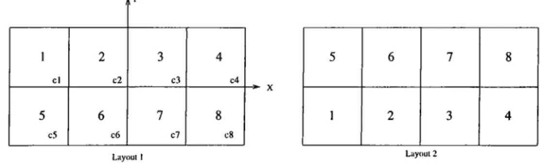
For example, for the 2x4 grid, Figure 1 shows two possible layouts where the squares represent the locations and numbers represent the machines (e.g. in Layout 2 machine 1 is located in the 5th location).

1 cl 2 c2 3 c3 4 c4 5 6 7 8 ^ X 5 6 7 8 1 2 3 4 c5 c6 c7 c8 Layout 1 Layout 2

Figure 2.1: Two possible layouts for 2x4

These two layouts which are symmetrical with respect to the x axis are distance invariant. Hence they are “the same layouts” with respect to the computations in our algorithm. For any given two row grid, by taking the symmetric with respect to the X axis, we can always find one other layout that is distance invariant. For a given three row grid, x axis is replaced by the middle row. Of course the same is true for two column (or three) grid and y axis (middle column).

In case the grid structure is cubic, the number of layouts that yield the same distance matrix increases to four which can be obtained by simultaneous perpendicular rotations. Due to the special structure of 2x2 and 3x3 grids, the number of distance invariant layouts is eight for them.

The set of all layouts can be partitioned into distance invariant classes. We can not computationally differentiate any of the layouts within each distance invariant class. Therefore we can perform the computations by taking arbitrarily one layout from each class which reduces the computations i o l j k where k is the cardinality of a distant invariant class. Note that the cardinality of each class is the same.

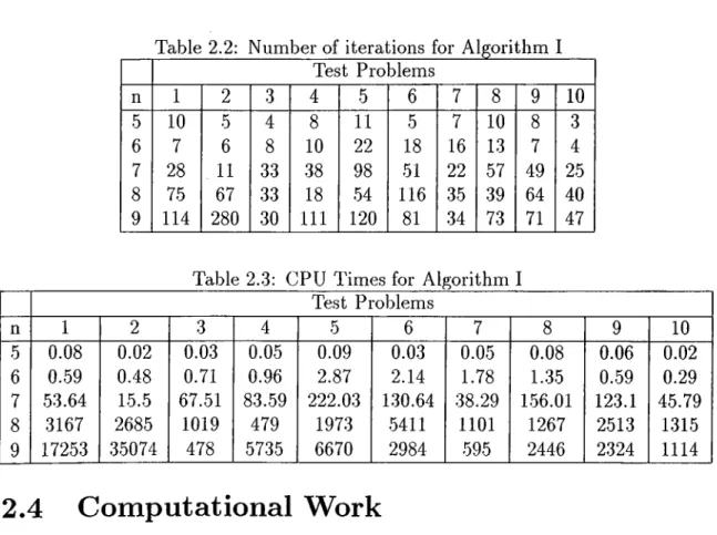
Table 2.1: Classification of the Layouts for the 3x3 Grid Group 1 Group 2 Group 3

1234 1243 1423 1324 1342 1432 2143 2134 2314 2413 2431 2341 3142 3124 3214 3412 3421 3241 4231 4213 4123 4321 4312 4132

For the 2x2 grid ?r! = 24 layouts can be classified into three groups such that layouts within each group, eight members each, have the same distance matrices. Table 2.1 shows this classification.

Suppose we select 1234, 1243, 1423, the first elements of each class in the Table 2.1. Figure 2.2 shows these layouts.

1 2 3 4 1 3 4 2 Layout 1 1234 Layout 2 1243 Layout 3 1423 Figure 2.2: Three layouts for the 2x2 grid that are not distance invariant

Consider Layout 1 and 2, only the following entries differ in their corresponding distance matrices.

¿13 — ¿31 — 1 ¿13 — ¿31 — 2 du = d\^ = 2 d\^ = d\^ = l

^23 ~ ^32 “ 2 <¿23 = <¿32 = 1

¿24 = ¿42 “ 1 ^24 “ ^42 “ ^

Define

Z}+^ = {¿ ¿ i : d i f = dij^ + 1} = {<^i3 , 4i,c?24,c?42}

= {dij ■ dij^ = dip + 1} = {¿14, ¿4 1, ¿23, <^42}

Then the maximum regret associated with selecting Layout 1 instead of Layout 2 is:

M i 2 ( l ,2 ) = wij~ - Y wij_ dijSDf^ dijSD'^2

In general, M R{k, 1) k and I € {1 ,2 ,3 } can be calculated from the following general formula:

M R{k, 1) — Y^ wij~ — Y^ wij _

then Maximum regret associated with each layout can be calculated as follows:

MR{1) = max(MR{l , 2), MRi l, 3) )

MR{2) = m ax{M R i2 ,1), M R {2 ,3))

MR{3) = 7nax{M Ri3,1), M R (‘S, 2)) And minimum regret solution is found by :

M in {M R (l), M R{2), MR{Z))

That means we can solve any 2x2 grid problem by solving six equations and four comparisons without using Algorithm I. Definitely as the size of the grid increases, the solution becomes complex. Still, the symmetry is of quite use. 3x3 grid case has the same properties as the 2x2 case (symmetry with respect to the axis and origin). This means that the cardinality of each distance invariant class is eight. This lowers the complexity by 1/8.

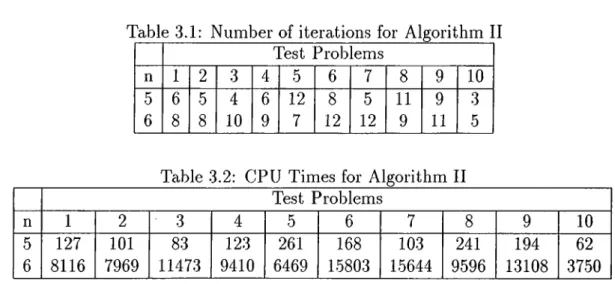
Table 2.2: Number of iterations for Algorithm I Test Problems n 1 2 3 4 5 6 7 8 9 10 5 10 5 4 8 11 5 7 10 8 3 6 7 6 8 10 22 18 16 13 7 4 7 28 . 11 33 38 98 51 22 57 49 25 8 75 67 33 18 54 116 35 39 64 40 9 114 280 30 111 120 81 34 73 71 47

Table 2.3: CPU Times for Algorithm I Test Problems n 1 2 3 4 5 6 7 8 9 10 5 0.08 0.02 0.03 0.05 0.09 0.03 0.05 0.08 0.06 0.02 6 0.59 0.48 0.71 0.96 2.87 2.14 1.78 1.35 0.59 0.29 7 53.64 15.5 67.51 83.59 222.03 130.64 38.29 156.01 123.1 45.79 8 3167 2685 1019 479 1973 5411 1101 1267 2513 1315 9 17253 35074 478 5735 6670 2984 595 2446 2324 1114

2.4

Computational Work

To test the performance of the proposed algorithm, ten test problems are generated for n € {5 ,6 ,7 ,8 ,9 } machines. Fixed flow amounts /¿j and percentages pij i = ,n } and j = are randomly generated in the interval [0,100]. then the upper and lower bounds for the flows are found as follows:

l U i j - = (1 - P i j/100) * f i j

% = ( 1 + P i j/100) * f i j

The layouts all of which have grid structures are given in Bl-5. Distance matrices are found using these grid structures and assuming rectilinear distances. Thus formed test problems are solved by using a C code on Sun Sparc Server lOOOE. Table 2.2 shows the number of iterations reached and Table 2.3 shows the CPU times in seconds. CPU times bigger than one thousand are rounded to nearest integers.

The number of iterations done in the iteration of Algorithm I can be found as follows:

Table 2.4: CPU Times for complete enumeration Test Problems n 1 2 3 4 5 6 7 8 9 10 5 0.34 0.39 0.37 0.37 0.37 0.37 0.38 0.37 0.37 0.37 6 28.33 28.27 28.31 28.31 28.34 28.31 28.37 28.32 28.3 28.29 7 3138 3139 3141 3142 3142 3139 3139 3139 3138 3138

In Step 2, approximately C {n,2) subtractions, multiplications, additions and comparisons are done for each possible assignment. Then the maximum is found by using n! comparisons, which makes 4n!(7(77,2) + n! operations.

Step 3 is a single comparison, hence we ignore it.

In Step 4, for a single assignment t times C{n,2) subtractions, multiplications and additions are done and t comparisons are performed to find the maximum of these quantities.This is repeated for each assignment and the minimum value is found by using n! comparisons. The total number of operations for Step 3 makes

i^C{n,2)t + t)n\ + n\.

Assuming T iterations are done until optimal is found, total number of operations for Algorithm I becomes T’?r![4C'(n, 2) + (3C'(n,2) + 1)(T + l ) /2 + 2]. On the other hand if complete enumeration were used, this number would be 4n!^C(n, 2) + nP as it would mean repeating Step 2 n\ times.

Using these total operation numbers, we compared Algorithm I and complete enumeration with the worst performing runs in Table 2.2: 7.5 and 9.2. In run 7.5 Algorithm I achieves a computational gain of 25.6% and in run 9.2; the gain increases to 91.7%. The relative computational performance of Algorithm I is expected to increase as the number of machines increases. However Algorithm I also becomes prohibitive with a large number of machines since it is also based on an enumeration

procedure. We also compared CPU times required for Algorithm I and complete enumeration. Table 2.4 shows the CPU times for complete enumeration for five, six and seven machines. For eight machines complete enumeration requires more than 48 hours, therefore it is no longer eflficient for more than seven machines.

It is also seen from Table 2.4 that CPU times for complete enumeration for a particular machine are very close to each other. However both the number of iterations required (Table 2.2) and CPU times (Table 2.3) for Algorithm I vary a lot. This is caused by the structural differences between the two methods. Complete enumeration covers all of the search space to find the optimal solution. However Algorithm I begins from an arbitrary assignment and covers some portion of the search space until the optimality condition is satisfied. The set of assignments covered is equal to the number of iterations done which is problem dependent. However note that even the largest number of iterations required is much less than the n! assignments covered by complete enumeration.