IMPROVED SOCIAL SPIDER ALGORITHM FOR MINIMIZING MOLECULAR POTENTIAL ENERGY FUNCTION
1Emine BAŞ , 2Erkan ÜLKER
1Selcuk University, Kulu Vocational School, Computer Technologies Department, Konya, TURKEY 2Konya Technical University, Engineering and Natural Sciences Faculty, Computer Engineering Department,
Konya, TURKEY
1[email protected], 2[email protected]
(Geliş/Received: 07.04.2019; Kabul/Accepted in Revised Form: 01.04.2020)
ABSTRACT: The social spider algorithm (SSA) is a new heuristic algorithm created on spider behaviors to solve continuous optimization problems. In this study, SSA is used in order to minimize a simplified model of the energy function of the molecule. The Molecular potential energy function problem is one of the most important real-life problems. The Molecular potential energy function problem attempts to predict the 3D structure of a protein. SSA is developed by various techniques (Crossover-mutation and Gbest convergence-silent spider techniques) and SSA is called Improved SSA (ISSA). By these techniques,
the exploration and exploitation capabilities of SSA in the continuous search space are improved. The general performances of SSA and ISSA are tested on low-scaled and large-scaled thirteen benchmark functions and obtained results are compared with each other. Wilcoxon signed-rank test is applied to SSA and ISSA results. Then, the general performance of the SSA and ISSA is tested on a simplified model of the molecule for different dimensions. Also, the performance of the ISSA is compared to various state-of-art algorithms in the literature. The results showed the superiority of the performance of ISSA.
Key Words: Constrained Optimization, Social spider algorithm, Molecular energy function
Moleküler Potansiyel Enerji Fonksiyonu İçin Geliştirilmiş Sosyal Örümcek Algoritması ÖZ: Sosyal örümcek algoritması (SÖA), sürekli optimizasyon problemlerini çözmek için örümcek davranışları üzerine oluşturulan yeni bir sezgisel algoritmadır. Bu çalışmada, SÖA molekülün enerji fonksiyonunun basitleştirilmiş bir modelini en aza indirmek için kullanılmıştır. Moleküler potansiyel enerji fonksiyonu problemi, en önemli gerçek hayat problemlerinden biridir. Moleküler potansiyel enerji fonksiyonu problemi, bir proteinin 3D yapısını tahmin etmeye çalışır. Sosyal örümcek algoritması çeşitli teknikler (Çaprazlama-mutasyon ve Gbest yakınsaması-sessiz örümcek teknikleri) eklenerek
geliştirilmiştir ve çeşitli tekniklerle geliştirilen SÖA 'ya Geliştirilmiş SSA (GSÖA) denilmiştir. Bu teknikler sayesinde, SÖA 'nın sürekli arama uzayında keşif ve sömürü yetenekleri geliştirilmiştir. SÖA ve GSÖA 'nın genel performansları, düşük ölçekli ve yüksek ölçekli on üç kıyaslama fonksiyonunda test edilmiştir ve elde edilen sonuçlar birbiriyle karşılaştırılmıştır. Wilcoxon işaretli testi, elde edilen SÖA ve GSÖA sonuçlarına uygulanmıştır. Daha sonra, SÖA ve GSÖA'nın genel performansı, farklı boyutlarda tanımlanan molekülün basitleştirilmiş bir modeli üzerinde test edilmiştir. Ayrıca, GSÖA'nın performansı, literatürdeki çeşitli sanatsal algoritmalarla da karşılaştırılmıştır. Sonuçlar, GSÖA 'nın performansının üstünlüğünü göstermiştir.
1. INTRODUCTION
Determining the global minimum potential energy conformation of proteins and peptides is known as the problem of energy minimization (Tawhid and Ali, 2017b). The minimization of the molecular potential energy function problem (MPEF) can be formulated as a global optimization problem. Finding the steady-state of the molecules in the protein can help to predict the 3D structure of the protein. The difficulty of the problem arises from the number of local minimizers of the energy function that grows exponentially with the size of the molecule (Wales and Scheraga, 1999). Many methods have been applied in the literature to solve this problem. Tawhid and Ali (2017a) proposed hybrid social spider optimization and genetic algorithm (HSSOGA) for MPEF. The social spider optimization (SSO) algorithm is a population-based algorithm proposed by Cuevas et al. (2013). SSO is another heuristic algorithm that is very similar to the SSA algorithm but different from it. Tawhid and Ali (2017b) proposed a hybrid Grey Wolf Optimizer and Genetic Algorithm (HGWOGA) for MPEF. The proposed HGWOGA algorithm is based on three procedures. In the first procedure, they apply the grey wolf optimizer algorithm with its powerful performance with the exploration and the exploitation processes and the second procedure is based on dimensionality reduction. The last procedure is to avoid premature convergence by applying the genetic algorithm mutation operator in the whole population. Tawhid and Ali (2017c) proposed hybrid flower pollination and genetic algorithm (HFPGA) and Tawhid and Ali (2016) improved a hybrid particle swarm optimization and genetic algorithm with population partitioning for large scale optimization problems for MPEF. Barbosa et al. (2005) proposed a steady-state real-coded genetic-simplex hybrid algorithm for MPEF. Pardalos et al. (1994) introduced some of the most commonly used potential energy functions and discuss different optimization methods used in the MPEF.
Yu and Li have offered Social Spider Algorithm (SSA) which is configured according to social spider behaviors (Yu and Li, 2015). Some spider species, which generally live solitary, can live as colonies. Spiders live in colonies can communicate with each other by web structure. The vibration they produce on the web enables this communication. They can make random walks to each other by the vibration information they share (Yu and Li, 2015). In this paper, we firstly propose an improved social spider algorithm (ISSA) and then ISSA is applied in order to solve the molecular potential energy function minimizations. Genetic algorithm operators are generally used in the literature to improve the exploration and exploratory ability of the algorithms. In this paper, we have added Gbest convergence
and silent spider techniques in addition to genetic algorithm operators. While crossover and Gbest
convergence techniques increase local search capacity of ISSA in continuous search space, mutation and silent spider techniques increase the global search capacity of ISSA in continuous search space. Crossover and Gbest convergence techniques have been used to escape the local minima trap. Mutation
and silent spider techniques ensure that global optimum points are found in the search space instead of local optimum points
.
The combination of these techniques accelerates the search and helps the algorithm to reach the optimal or near-optimal solution in a reasonable time. In this paper, the ISSA has been tested on various thirteen low-scaled and large-scaled benchmark functions. The molecular potential energy problem is solved by ISSA in various dimensions and the performances of ISSA are compared with well-known algorithms in the literature.The general structure of the paper as follows. The related works and the definition of the molecular energy problem are details presented in section 1 and 2, respectively. In section 3, the original SSA and in section 4, ISSA is examined. In section 5, original SSA and ISSA are tested in various unimodal and multimodal benchmark functions in low-scale and large-scale dimensions. The performance of the SSA and ISSA is tested on a simplified model of the molecule with different dimensions. Obtained results are compared with each other and well-known heuristic and new methods in the literature. Finally, the results are interpreted and discussed. The paper is ended up with a conclusion and future works.
2. RELATED WORKS
Evolutionary computation has become an attractively efficient device of optimization for rapidly increasing complex modern optimization problems. For the last twenty years, swarm intelligence based algorithms, which are based on new evolutionary computation methods, attract attention. The term of a swarm expresses a community that consists of individuals who are in communication with each other. Swarm intelligence-based algorithms, study main social animal and insect behaviors for solving problems. These algorithms, imitate the behaviors of ant, fish, bird, bee, bacteria, butterfly, etc. Thus, the problems which seem hard are able to be solved (Talbi, 2009; Mallipeddi et al., 2011; Parpinelli and Lopes, 2011; Kennedy and Eberhart, 1995).
One of the most popular heuristic algorithms in the literature is GA. GA has crossover and mutation operators (Holland, 1975). These operators have been used effectively in a variety of heuristic algorithms. Particle swarm optimization (PSO) is one of the most hybrid algorithms with GA. For example, GA–PSO and PSOGA (Robinson et al., 2002) which are solved he particular electromagnetic application of profiled corrugated horned antenna, GSO (Grimaldi et al., 2004) which is solved combinatorial optimization problems, GSO with several strategies (Grimaccia et al., 2007) which is solved some multi-modal benchmark problems, and BS (Settles and Soule, 2005) which is resolved unconstrained optimization problems. In addition, there are many studies in the literature that have been hybridized with GA operators (Krink and Lvbjerg, 2002; Juang, 2004; Jian and Chen, 2006).
In this paper, one of the heuristic methods, the social spider algorithm has been selected. With the vibrations in SSA are shared some information in continuous spaces and the spiders are socialized at the evolutionary process. In the literature, SSA has been used in various papers. El-bages and Elsayed (2017) have solved a static transmission expansion planning problem by using SSA. In the proposed method; DC power flow sub-problem is solved by developing an original SSA based web and adding potential solutions to the result. Yu and Li (2016) have solved the Economic Load Dispatch (ELD) formulation by developing an original SSA based new approach. ELD is one of the essential components in power system control and operation. Mousa and Bentahar (2016) have adapted QoS-aware web service selection process to OSSA approach. Elsayed et al. (2016) have solved the non-convex economic load dispatch problem with an OSSA based approach.
3. MOLECULAR POTENTIAL ENERGY PROBLEM
We test on a scalable simplified molecular potential energy function (MPEF) to examine the performance of ISSA. MPEF is first proposed in (Lavor and Maculan, 2004). The potential energy of a molecule is derived from molecular mechanics, which describes molecular interactions based on the principles of Newtonian physics (Tawhid and Ali, 2017).
The molecular model has formed consists of a chain of k atoms (a1, a2, …, ak) in a
three-dimensional space. Similar models have been figured in the literature (Hedar et al., 2011; Bansal et al., 2010). In this paper, we define the potential energy as a function of the torsion angles as Equation 1.
E = ∑ (1 + Cos(3ωi,i+3) +
(−1)i
√10.60099896−4.141720682(cos(ωi,i+3)))
i (1)
where i = 1, . . . ,k−3 and k is the number of atoms in the given model and ωi, i + 3 is the torsion angle by the atoms ai, ai+1, ai+2 and ai+1, ai+2, ai+3. Figure 1 is shown in the torsion angle.
ai
ai+1
ai+2
ai+3
Figure 1. The torsion angle between the normal through the planes determined by the atoms ai, ai+1, ai+2,
and ai+1, ai+2, ai+3.
Our goal is to find ω1,4, ω2,5, . . . , ωk−3, k where ωi, j ∈ [0, 5]. Although the problem seems simple, it
is a very difficult problem. A molecule with as few as 20 atoms has 217 = 131.072 local minimizers.
In this paper, E is rewritten as f (x) for the large-scale unconstrained global optimization problem. Equations 2-4 show fitness function.
f(x) = ∑ (1 + Cos(3xi) + (−1)i
√10.60099896−4.141720682(Cos(xi))) n
i=1 (2)
And 0 ≤ xi ≤ 5,i = 1, … , n (3) min f(x),x ∈ Rn l
b≤ xi ≤ ubi = 1, 2, … , n (4) where f: Rn → R is an objective function and x represents a decision variable vector. l
b and ubare the lower and upper bounds of the decision variables xi, respectively.
4. ORIGINAL SOCIAL SPIDER ALGORITHM (SSA)
Social spider algorithm (SSA) is a heuristic algorithm that is created by imitating spiders’ behaviors in nature. SSA is created for organizing searching space of optimization problems as a high dimensional spider web. Each position on the web represents a convenient solution for the optimization problem and all convenient solutions to the problem correspond to positions on this web. This web also serves as a transmission medium of vibrations created by spiders. Each spider on the web is held in a position and the conformity value of the solution is calculated with the objective function. Spiders can move randomly on the web. But they can not move out of positions which represent convenient solutions for optimization problems. When a spider moves towards a new position, a vibration is produced and this vibration spreads on the web. Other spiders execute social information sharing via this vibration. Flowchart for the original SSA is shown in Figure 2.
Figure 2. Flowchart For SSA
There are two important terms in SSA: spider and vibration. Spider structure: Spiders are SSA agents that perform optimization. At the beginning of the algorithm, a predetermined number of spiders are placed on the web. The number of spiders cannot be changed afterward. “a” represents a spider and a memory is allocated for each spider a. Spider information is stored here. This information: the position of spider a on the web, the fitness value at the current position of spider a, the target vibration of spider a in the previous iteration, the iteration number where the target vibration last changed, the movement of spider a in the previous iteration and the dimension mask of spider a that guided the movement in the previous iteration. Spider locations are initially set at random. Each spider produces a vibration when it moves from a position to a different location. The severity of the vibration is related to the fitness value that the spider produces in that position. Vibration can spread over the web and other spiders on the web can feel it. Thus, other spiders on the web can obtain the personal information of the spider that produces the vibration, and information sharing takes place. Vibration structure: The vibration in the SSA is a very important term. It is one of the most important characteristics distinguishing SSA from other meta-heuristic algorithms. Two properties are used to define a vibration. a-) The source position b-) The source of vibration severity [0,+ ∞) Equation 5 (Yu and Li, 2015) is used to calculate the vibration intensity.
I(Pa, Pa, t) = log ( 1
f(pa)−C) +1 (5) Where a represents a spider and spider a generates vibration at its current position. It defines the position of spider a at time t as Pa(t), or simply as Pa if the time argument is t. Where I( Pa, Pa, t) is the
Iteration <= Max_iteration
Fitness evaluation
Spider vibration generation
Spider binary mask changing
Perform a random walk for each spider
Final Initialization
Create random continuous space, Assign values to the parameters
Yes No
vibration value produced by the spider in the source position at time t. f(Pa) represents the spider of
fitness value in its current position. Where C is a confidently small constant such that all possible fitness values are larger than C for minimization problems. Dis( Pa, Pb) is showing the distance between spider a
and spider b. This distance is calculated by Equation 6 (Yu and Li, 2015). Manhattan distance structure is used when calculating this distance. The vibration attenuation over distance is calculated by Equation 7 (Yu and Li, 2015).
𝐷𝑖𝑠(𝑃𝑎, 𝑃𝑏) = ‖𝑃𝑎 − 𝑃𝑏‖ (6) 𝐼(𝑃𝑎, 𝑃𝑏, 𝑡) = 𝐼(𝑃𝑎, 𝑃𝑎, 𝑡) × 𝑒𝑥𝑝 (−𝐷𝑖𝑠(𝑃𝑎,𝑃𝑏)
𝜎̅×𝑟𝑎 ) (7)
Where σ̅ represents mean of the standard deviation of the positions of all spiders in each dimension. ra is represented as a user-controlled parameter ra ∈ (0, ∞ ). This parameter controls the
attenuation rate of the vibration intensity over the distance. Whenever a spider moves to a new position, it generates vibration at its current position. I(Pa,Pb,t) is the felt value of the spider’s vibration in “a”
point, by the spider in “b” point. The value of ra is selected from the set {1/10, 1/5, 1/4, 1/3, 1/2, 1, 2, 3, 4, 5,
10} and the values of pc and pm are both selected from the set {0.01, 0.1, 0.2, 0.3, 0.4, 0.5, 0.6, 0.7, 0.8, 0.9,
0.99} (Yu and Li, 2015). After setting the values, the algorithm creates an initial population of spiders for optimization. Each spider is assigned a fixed size memory for storing spider information. The positions of spiders are randomly generated in the search space. Fitness values of the spiders calculated and stored. The initial target vibration of each spider in the population is set at its current position, and the vibration intensity is zero. All spiders produce vibration using their position. The algorithm uses vibrations to activate the propagation process. V represents spiders' vibrations. Each spider receives the vibrations generated by other spiders. A spider selects the strongest of these vibration values. This value shows as Vabest, a represents a spider. Spider a which is stored in the memory of the target vibration
shows as Vatar. Vabest compares vibration values and if the intensity of the Vabest is not greater than the
target vibration, the spider's memory is changed to Vabest. cs, the number of iterations since spider a has
last changed its target vibration, is reset to zero; otherwise, the original Vatar is retained and cs is
incremented by one. The dimension mask m is determined so that a random walk can be performed towards the Vatar. The dimension mask is a {0, 1} binary vector of length n and n is the dimension of the
optimization problem. Initially, all the values of this mask are zero. In each iteration, spiders have a probability of 1 – pccs to change its mask where pc∈ (0, 1) is a user-defined attribute that describes the
probability of changing mask. If the mask is decided to be changed, each bit of the vector has a probability of pm to be assigned with a one, and 1 – pm to be a zero. Pm is also a user-controlled
parameter defined in (0, 1) (Yu and Li, 2015). Each bit of the mask is changed independently. The new mask does not have any correlation with the previous mask. In case all bits are zeros or ones, one random value of the mask is changed to one or zero. After the dimension mask is determined, a new following position Pafo is generated based on the mask for a spider. Pafo value is calculated by Equation 8
(Yu and Li, 2015).
𝑃𝑎,𝑖𝑓𝑜 = {𝑃𝑎,𝑖 𝑡𝑎𝑟, 𝑚
𝑎,𝑖= 0 𝑃𝑎,𝑖𝑟 , 𝑚𝑎,𝑖= 1
(8)
Where r is a random integer value generated in [1, population_size] and ma,i stands for the ith
dimension of the dimension mask m of spiders. The random walk of each spider is calculated by Equation 9 (Yu and Li, 2015).
𝑃𝑎(𝑡 + 1) = 𝑃𝑎+ (𝑃𝑎− 𝑃𝑎(𝑡 − 1)) × 𝑟 + (𝑃𝑎 𝑓𝑜
Where ʘ denotes element-wise multiplication. R is a vector of random float-point numbers generated from zero to one uniformly. Before following Pafo, spider a first moves along its previous
direction, which is the direction of movement in the previous iteration. The distance along this direction is a random portion of the previous movement. Then spider a approaches Pafo along each dimension
with random factors generated in (0, 1). After each spider performs a random walk, the spiders may move out of the web. It blocks the constraints of the optimization problem to be violated. The work steps of the original SSA is shown in Figure 3.
Step 1. Parameter setting: Required constant parameter sets are adjusted. For example, lower and upper limits of variables, number of maximum iteration, etc.
Step 2. Initialization: Random starting position locations are determined for each spider in the swarm. Assign memory for them. The target vibration for each spider is started.
Step 3. Evaluation: Fitness value is calculated for each spider. The best in the swarm are detected and recorded.
Step 4. Vibration value for each spider calculated by using vibration Equations (5, 6, and 7). The best in the swarm are detected and recorded.
Step 5. Vibration comparison: The received the best vibration is compared to the target vibration values. Step 6. Update the dimension mask.
Step 7. Pafo value is calculated by Equation 8
Step 8. Movement: Each spider moves to a new position by Equation 9 and a new population is obtained. Step 9. Repeat: All criteria beginning from Step 3 are repeated until reaching stopping criteria.
Step 10. Output: Optimum outputs are obtained.
Figure 3. The work steps of the original SSA
5. IMPROVED SOCIAL SPIDER ALGORITHM (ISSA)
The original SSA is an optimization algorithm that is developed for solving constant problems. In this paper, SSA is studied and it is improved by adding new four techniques enhancing its performance (ISSA). These techniques are crossover, mutation, Gbest convergence, and silent spider
techniques. In both techniques, ISSA develops the ability to search locally and globally in continuous search space. While crossover and Gbest convergence techniques increase local search capacity of ISSA in
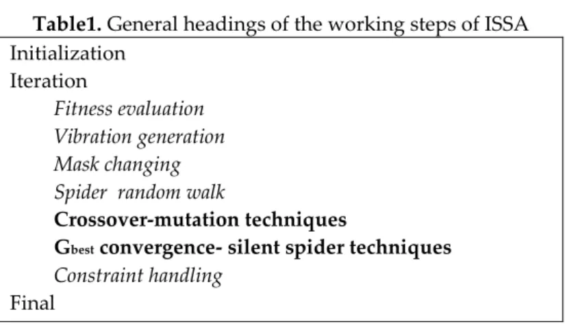
continuous search space, mutation and silent spider techniques increase the global search capacity of ISSA in continuous search space. The working steps of ISSA are shown in Table 1 with general headings and details. In this Table, newly added to original SSA steps are indicated by bold letters. Fitness evaluation, vibration generation, mask changing, and spider random walk steps are taken from SSA and used similarly in ISSA.
Table1. General headings of the working steps of ISSA Initialization Iteration Fitness evaluation Vibration generation Mask changing Spider random walk
Crossover-mutation techniques
Gbest convergence- silent spider techniques Constraint handling
Final
Crossover-mutation Schema: ISSA is avoided trapped around the local point with crossover and mutation operators. The value of crossover rate (cr) and the mutation rate (mr) is selected from the set {10%, %20, 30%, 40%, 50%, 60%, 70%, 80%, 90%}. The most appropriate cr value was found to be 90%. The most appropriate mr value was found to be 10%. Let N be the number of the population size, n show the dimension of the population; Figure 4 is shown in the crossover process. Figure 5 is shown in the mutation process.
Lets n=10, cr=90, Round(n*90)/100= 9 N=1.spider 0 1 1 1 1 0 1 1 0 1 rand(N)=5.spider 1 0 0 1 0 0 1 0 0 0
Nnew spider in crossover process
1 0 0 1 0 0 1 0 0 1
Figure 4. Crossover process Lets n=10, mr=10, Round(n*10)/100= 1
Nnew spider in crossover process
1 0 0 1 0 0 1 0 0 1
Nnew spider in mutation process
1 0 0 1 1 0 1 0 0 1
Figure 5. Mutation process
Gbest convergence Schema: The Gbest convergence rate (gr) is selected from the set {10%, %20,
30%, 40%, 50%, 60%, 70%, 80%, 90%}. The most appropriate gr value was found to be 40%. The Gbest
convergence improves the ability of ISSA to search locally in continuous space. Let N be the number of the population size, n show the dimension of the population; Figure 6 is shown Gbest convergence
process.
crossover
Lets n=10, gr=40, Round(n∗40)/100= 4 N=Global best spider in population
1 1 1 0 0 0 0 1 1 1
N=1.spider
0 1 1 1 1 0 1 1 0 1
Nnew spider in Gbest convergence process
0 1 1 1 0 0 0 1 1 1
Figure 6. Gbest convergence process
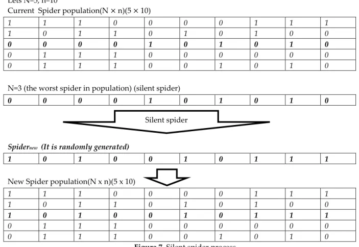
Silent spider Schema:The worst spider (silent spider) in the original SSA is hidden throughout each iteration. This spider has a small effect on the optimum result. ISSA has determined and omitted the worst spider (silent spider) and has added a new random spider (spidernew) which can possibly have
more effect on the optimum result. The fitness value of the new spider is controlled while adding it. If the fitness value of the new spider is worse than the fitness value of the worst spider (silent spider) of the population, it is never added to the population. The system preserves existing population members. If the fitness value of the new spider is better than the fitness value of the worst spider (silent spider) of the population, the silent spider is omitted from the population and a new spider is replaced (spidernew).
So, a predetermined fixed population amount is preserved. This process is repeated throughout each iteration. Figure 7 is shown a silent spider process.
Lets N=5, n=10
Current Spider population(N × n)(5 × 10)
1 1 1 0 0 0 0 1 1 1
1 0 1 1 0 1 0 1 0 0
0 0 0 0 1 0 1 0 1 0
0 1 1 1 0 0 0 0 0 0
0 1 1 1 0 0 1 0 1 0
N=3 (the worst spider in population) (silent spider)
0 0 0 0 1 0 1 0 1 0
Spidernew (It is randomly generated)
1 0 1 0 0 1 0 1 1 1
New Spider population(N x n)(5 x 10)
1 1 1 0 0 0 0 1 1 1
1 0 1 1 0 1 0 1 0 0
1 0 1 0 0 1 0 1 1 1
0 1 1 1 0 0 0 0 0 0
0 1 1 1 0 0 1 0 1 0
Figure 7. Silent spider process
Figure 8 shows a flowchart of ISSA and Figure 9 shows pseudocode of the ISSA. Silent spider
Figure 8. Flowchart For ISSA Iteration <= Max_iteration
Fitness evaluation
Spider vibration generation
Silent spider Technique
Spider binary mask changing
Final Initialization
Create random continuous space
Crossover-Mutation Technique Yes
No
1: 2: 3: 4: 5: 6: 7: 8: 9: 10: 11: 12: 13: 14: 15: 16: 17: 18: 19: 20: 21: 22: 23: 24: 25: 26: 27: 28:
Assign values to the parameters of ISSA
Create the population of spiders N, assign memory for them Initialize Vatar for each spider
while stopping criteria not met do
Apply the original social spider algorithm on all populations. Select Silent spider in population
Generate a new spider as spidernew
if spidernew fitness value is smaller than Silent spider fitness value then
Update Silent spider as spidernew
end if
for each spider s in spider population do Select random r spider in spider population
Apply the crossover process between s and r spider according to crossover rate and get the new spider(spidernew1)
Apply mutation process on spidernew1 according to mutation rate and get the new
spider(spidernew2)
if spidernew2 fitness value is smaller than s spider fitness value then
Update s spider as spidernew2
end if end for
for each spider s in spider population do
Select Gbest spider(Global best spider) in population
Apply Gbest convergence process between Gbest and s spider according to Gbest
convergence rate and get the new spider(spidernew)
if spidernew fitness value is smaller than s spider fitness value then
Update s spider as spidernew
end if end for
Address any violated constraints end while
Output the best solutions found
Figure 9. Pseudocode of the ISSA 6. EXPERIMENTAL RESULTS AND ANALYSIS
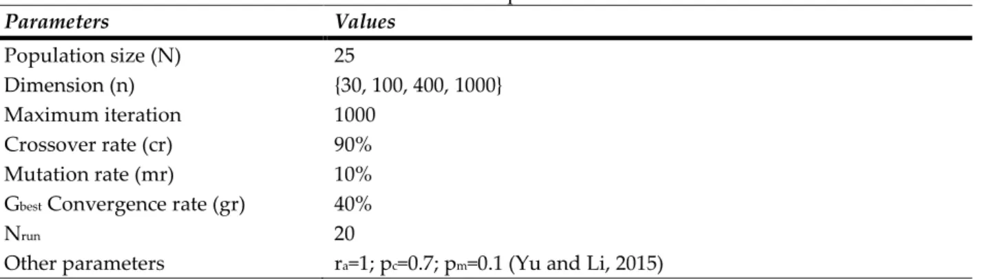
ISSA and SSA are tested on Matlab R2014a that installed over windows 7, 64 bit, the system of 2.30 GHz processor with 4GB RAM. Common parameters used in ISSA and SSA comparison, which are population size (N), dimension (n), maximum iteration values, ra value, pc value, pm value, crossover rate
(cr), mutation rate (mr), and Gbest convergence rate (gr) are shown in Table 2. The values of ra, pc, pm are
taken directly from SSA. The values of cr, mr, and gr are selected from the set {10%, 20%, 30%, 40%, 50%, 60%, 70%, 80%, 90%}. In experimental studies, thirteen different unimodal and multimodal benchmark functions, which are shown in Table 3 with ISSA and SSA, are solved separately. The performance of ISSA is solved on both the global optimization problems and molecular potential energy problems, respectively. Silent Spider Technique Crossover Technique And Mutation Technique Gbest convergence Technique
Tablo 2. Parameters setup for ISSA and SSA Parameters Values Population size (N) 25 Dimension (n) {30, 100, 400, 1000} Maximum iteration 1000 Crossover rate (cr) 90% Mutation rate (mr) 10%
Gbest Convergence rate (gr) 40%
Nrun 20
Other parameters ra=1; pc=0.7; pm=0.1 (Yu and Li, 2015)
Table 3. Classical Benchmark functions used in the experimental study.
Type Name Function Range fminimum
Unimodal F1 ∑ 𝑥 𝑖2 𝑛 𝑖=1 [-100,100]n f(X*)=0 F2 ∑ |𝑥 𝑖| 𝑛 𝑖=1 + ∏ |𝑥𝑖| 𝑛 𝑖=1 [-10,10]n f(X*)=0 F3 ∑ (∑ 𝑥𝑗 𝑖 𝑗=1 ) 2 𝑛 𝑖=1 [-100,100]n f(X*)=0 F4 𝑚𝑎𝑥𝑖|𝑥𝑖|,1 ≤ 𝑖 ≤ 𝑛 [-100,100]n f(X*)=0 F5 ∑ [100(𝑥𝑖+1− 𝑥𝑖2) 2 + (𝑥𝑖− 1)2] 𝑛−1 𝑖=1 [-30,30]n f(X*)=0 F6 ∑([𝑥𝑖+ 0.5])2 𝑛 𝑖=1 [-100,100]n f(X*)=0 F7 ∑ 𝑖𝑥𝑖4 𝑛 𝑖=1 + 𝑟𝑎𝑛𝑑𝑜𝑚[0,1) [-1.28,1.28]n f(X*)=0 Multimodal F8 ∑ −𝑥𝑖 𝑛 𝑖=1 𝑠𝑖𝑛 (√|𝑥𝑖|) [-500,500]n f(X*)=−418.9829 × n F9 ∑[𝑥𝑖2− 10𝑐𝑜𝑠(2𝜋𝑥𝑖) + 10] 𝑛 𝑖=1 [-5.12,5.12]n f(X*)=0 F10 −20𝑒𝑥𝑝 (−0.2√1 𝑛∑ 𝑥𝑖 2 𝑛 𝑖=1 ) − 𝑒𝑥𝑝 (1 𝑛∑ 𝑐𝑜𝑠(2𝜋𝑥𝑖) 𝑛 𝑖=1 ) + 20 + 𝑒𝑥𝑝(1) [-32,32]n f(X*)=0 F11 1 4000∑ 𝑥𝑖 2− ∏ 𝑐𝑜𝑠 (𝑥𝑖 √𝑖) 𝑛 𝑖=1 𝑛 𝑖=1 +1 [-600,600] n f(X*)=0 F12 1 − 𝑐𝑜𝑠 (2𝜋√∑ 𝑥𝑖2 𝑛 𝑖=1 ) + 0.1√∑ 𝑥𝑖2 𝑛 𝑖=1 [-100,100]n f(X*)=0 F13 − ∑ 𝑠𝑖𝑛(𝑥𝑖) 𝑛 𝑖=1 𝑠𝑖𝑛2𝑚(𝑖𝑥𝑖 2 𝜋) [0,π]n n=30: f(X*)=-29,6309; n=100: f(X*)= -99.6201940166; n=400: f(X*)= -399,616795138572; n=1000: f(X*)= -999.6161052093
Benchmark functions divide into two groups according to their type as unimodal and multimodal benchmark functions. Functions F1-F7 (unimodal), which have only one global optimum
and can evaluate the exploitation capability of the investigated algorithms. Functions F8–F13 (multimodal), which include many local optima whose number increases exponentially with the problem size, become highly useful when the purpose is to evaluate the exploration capability of the investigated algorithms. These functions are obtained from various sources (Tawhid and Ali, 2017a; Yu and Li, 2015; Surjanovic and Bingham, 2017).
For each benchmark function, two measures are used to evaluate the performance of each algorithm to solve this function. These measures include (1) Average ( Mean ) and (2) Standard deviation ( S.D.). They defined as in Table 4. Where Nrun represents the total number of runs.
Table 4. Performance measure Mean Mean = 1 Nrun × ∑ Fitness_funci Nrun i=1 Standard Deviation S. D. = √ 1 Nrun ∑ (Gbesti− Mean)2 Nrun i=1
6.1. Determine of crossover, mutation, and Gbest convergence rates
To determine the crossover rate (cr), population size = 25, dimension=30 and maximum iteration = 1000 parameter values are selected for ISSA. The crossover rate (cr) is tested in randomly selected five different unimodal benchmark functions (F1, F2, F4, F5, and F7) and randomly selected five different multimodal benchmark functions (F8, F9, F10, F11, and F13). Each benchmark function is run 20 times. Mean are done for obtained benchmark function results. Table 5 shows the results obtained. According to the results, the crossover rate (cr) is selected at 90%.
Table 5. Determine the crossover rate (cr) in 10 different unimodal and multimodal benchmark functions. F Crossover rate (cr) 10% 20% 30% 40% 50% 60% 70% 80% 90% F1 27004,4900 26156,1900 17520,1100 18324,9400 10140,2200 8790,2180 7135,4120 3347,9670 1175,5600 F2 66,20135 69,99781 55,3307 53,31256 35,07983 37,10695 20,20037 22,91025 11,5507 F4 49,85766 45,78515 35,00857 28,66598 22,04498 21,00766 19,00288 20,91694 19,2189 F5 47536115 30431267 20364778 9716929 5907726 2776247 970753,500 1060099 38362,99 F7 0,0000 0,0000 0,0000 0,0000 0,0000 0,0000 0,0000 0,0000 0,0000 F8 -3112,3900 -2690,1100 -2947,0400 -2547,1600 -3073,5100 -2572,2100 -3227,9500 -2949,1200 -2693,3300 F9 244.9703 257,9103 188,5917 152.5475 112,2209 92,60459 64,57314 42,30282 36,73263 F10 18,92449 17,49768 17,00651 17,20581 15,78174 14,79526 13,53442 11,89024 10,78819 F11 283,2028 232,6389 188,1118 146,7355 84,3342 78,03849 54,26156 23,68114 9,374057 F13 -8,78887 -9,00019 -8,67862 -9,16455 -8,73005 -9,33821 -8,90599 -9,10591 -9,18917
To determine the mutation rate (mr), population size = 25, dimension=30 and maximum iteration = 1000 parameter values are selected for ISSA. The mutation rate (mr) is tested in randomly selected five different unimodal benchmark functions (F1, F2, F4, F5, and F7) and randomly selected five different multimodal benchmark functions (F8, F9, F10, F11, and F13). Each benchmark function is run 20 times. Mean are done for obtained benchmark function results. Table 6 shows the results obtained. According to the results, the mutation rate (mr) is selected at 10%.
Table 6. Determine the mutation rate (mr) in 10 different unimodal and multimodal benchmark functions. F Mutation rate (mr)
10%
20% 30% 40% 50% 60% 70% 80% 90% F1 0,394634 0,702821 0,758151 0,617514 0,702059 0,671051 0,751396 0,905282 0,814592 F2 0,141074 0,134244 0,168751 0,210592 0,1827 0,199393 0,208086 0,208631 0,187357 F4 18,04599 21,89031 23,99734 24,45129 26,38615 25,51669 25,80048 24,79854 25,72667 F5 282,6736 313,285 327,3802 383,4963 331,8956 429,427 360,3212 383,9664 424,8467 F7 0,0000 0,0000 0,0000 0,0000 0,0000 0,0000 0,0000 0,0000 0,0000 F8 -3325,990 -4201,030 -4000,200 -4730,400 -4522,850 -5123,600 -4961,060 -4514,820 -4711,540 F9 56,78534 53,34603 49,45195 46,10922 45,66494 47,71347 50,04745 45,39075 46,79847 F10 0,267519 0,316517 0,354352 0,340763 0,364685 0,317098 0,30045 0,390763 0,412149 F11 0,679518 0,745935 0,752064 0,819712 0,825792 0,84922 0,777499 0,923743 0,826685 F13 -8,9389 -9,15235 -9,13946 -8,75084 -9,03193 -9,09553 -9,04802 -9,04717 -8,79987To determine the Gbest convergence rate (gr), population size = 25 and maximum iteration = 1000
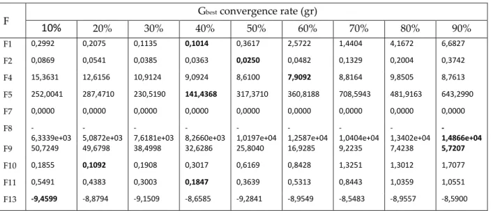
parameter values are selected for ISSA. The Gbest convergence rate (gr) is tested in randomly selected five
different unimodal benchmark functions (F1, F2, F4, F5, and F7) and randomly selected five different multimodal benchmark functions (F8, F9, F10, F11, and F13). Each benchmark function is run 20 times. Mean are done for obtained benchmark function results. Table 7 shows the results obtained. According to the results, the convergence rate (gr) is selected at 40%.
Table 7. Determine the Gbest convergence rate (gr) in 10 different unimodal and multimodal benchmark
functions.
F G
best convergence rate (gr)
10%
20% 30% 40% 50% 60% 70% 80% 90% F1 0,2992 0,2075 0,1135 0,1014 0,3617 2,5722 1,4404 4,1672 6,6827 F2 0,0869 0,0541 0,0385 0,0363 0,0250 0,0482 0,1329 0,2004 0,3742 F4 15,3631 12,6156 10,9124 9,0924 8,6100 7,9092 8,8164 9,8505 8,7613 F5 252,0041 287,4710 230,5190 141,4368 317,3710 360,8188 708,5943 481,9163 643,2990 F7 0,0000 0,0000 0,0000 0,0000 0,0000 0,0000 0,0000 0,0000 0,0000 F8 -6,3339e+03 -5,0872e+03 -7,6181e+03 -8,2660e+03 -1,0197e+04 -1,2587e+04 -1,0404e+04 -1,3402e+04 -1,4866e+04 F9 50,7249 49,6798 38,4998 32,6286 25,8040 16,9285 9,2235 7,4238 5,7207 F10 0,1855 0,1092 0,1908 0,3017 0,6169 0,8428 1,3251 1,3012 1,7077 F11 0,5491 0,4383 0,3003 0,1847 0,3639 0,5313 0,8443 1,0359 1,0551 F13 -9,4599 -8,8794 -9,1509 -8,6585 -9,2841 -8,9549 -8,5483 -8,9557 -8,59006.2. The contribution of crossover (cr), mutation (mr), Gbestconvergence (gr), and silent spider
techniques to the proposed algorithm
Each developed technique is applied individually with ISSA and its contribution to ISSA has been demonstrated. Each benchmark function is run 20 times. Mean and standard deviation (S.D.) are done for obtained benchmark function results. The results are shown in Tables 8 and 9. According to obtain results, all techniques have improved ISSA's local and global search capabilities. Gbestconvergence
and silent spider techniques are had good performance except for F5 and F6. Gbestconvergence and silent
spider techniques have improved ISSA's local and global search capabilities. Crossover and mutation techniques are had sufficiently good performance except for F8, F12, and F13.
Table 8. The comparison of ISSA with cr, mr, gr, and silent spider techniques on dimension = {30}, the maximum number of iterations = 1000 in unimodal and multimodal benchmark functions.
F
ISSA
cr mr gr silent spider
Mean S.D. Mean S.D. Mean S.D. Mean S.D. F1 0,00E+00 0,00E+00 0,00E+00 0,00E+00 0,00E+00 0,00E+00 0,00E+00 0,00E+00 F2 0,00E+00 0,00E+00 0,00E+00 0,00E+00 0,00E+00 0,00E+00 0,00E+00 0,00E+00 F3 0,00E+00 0,00E+00 0,00E+00 0,00E+00 0,00E+00 0,00E+00 0,00E+00 0,00E+00 F4 0,00E+00 0,00E+00 0,00E+00 0,00E+00 0,00E+00 0,00E+00 0,00E+00 0,00E+00 F5 178,9085 60,0856 177,8799 60,6647 183,7258 96,9333 231,9934 79,9607 F6 15,7213 6,7661 14,1819 4,1252 14,2264 4,1434 14,1882 4,1691 F7 0,00E+00 0,00E+00 0,00E+00 0,00E+00 0,00E+00 0,00E+00 0,00E+00 0,00E+00 F8 -4,37e+03 8359,600 -3,29e+03 7960,018 -6,47e+03 4730,590 -6,60e+03 2650,303 F9 0,00E+00 0,00E+00 0,00E+00 0,00E+00 0,00E+00 0,00E+00 0,00E+00 0,00E+00 F10 6,18e-10 0,00E+00 6,18e-10 0,00E+00 8,88e-16 0,00E+00 8,88e-16 0,00E+00 F11 0,00E+00 0,00E+00 0,00E+00 0,00E+00 0,00E+00 0,00E+00 0,00E+00 0,00E+00 F12 0,6215 0,2514 11,7313 1,4812 0,1203 0,2302 0,3289 0,6639 F13 -8,4004 0,7053 -8,4930 0,7034 -8,7114 0,6902 -9,0613 0,6941
Table 9. The comparison of ISSA with cr-mr, and gr-silent spider techniques on dimension = {30}, the maximum number of iterations = 1000 in unimodal and multimodal benchmark functions.
F
ISSA
cr-mr gr-silent spider
Mean S.D. Mean S.D.
F1 0,00E+00 0,00E+00 0,00E+00 0,00E+00 F2 0,00E+00 0,00E+00 0,00E+00 0,00E+00 F3 0,00E+00 0,00E+00 0,00E+00 0,00E+00 F4 0,00E+00 0,00E+00 0,00E+00 0,00E+00 F5 177,8799 60,0856 180,71421 66,4571 F6 13,1852 3,8091 14,1852 4,7590 F7 0,00E+00 0,00E+00 0,00E+00 0,00E+00 F8 -5,10e+03 3730,5997 -6,60e+03 2650,303 F9 0,00E+00 0,00E+00 0,00E+00 0,00E+00 F10 8,18e-15 0,00E+00 8,88e-16 0,00E+00 F11 0,00E+00 0,00E+00 0,00E+00 0,00E+00 F12 0,00E+00 0,00E+00 0,00E+00 0,00E+00
6.3. The general performance of the ISSA and SSA on low-scaled and large-scale optimization problems
ISSA is tested in seven unimodal benchmark functions. Each benchmark function is run 20 times. Mean and standard deviation (S.D.) are done for obtained benchmark function results. Mean and standard deviation (S.D.) comparison results, which are obtained for unimodal benchmark functions (F1-F7) by selecting population size (N) =25 and maximum iteration=1000 values for ISSA, are shown in Table 10. According to obtain results, ISSA is had super performance except for F5 and F6.
Table 10.The performance of ISSA with dimension = {30, 100, 400, 1000}, maximum number of iterations = 1000, population size = 25 in unimodal benchmark functions. S.D. is the standard deviation;
Mean is the average of the unimodal benchmark function results.
F1 F2 F3 F4 F5 F6 F7
30 Mean 0,00E+00 0,00E+00 0,00E+00 0,00E+00 1,78E+02 1,29E+01 0,00E+00 S.D. 0,00E+00 0,00E+00 0,00E+00 0,00E+00 6,16E+01 3,59E+00 0,00E+00 100 Mean 0,00E+00 0,00E+00 0,00E+00 0,00E+00 3,15E+04 9,04E+01 0,00E+00 S.D. 0,00E+00 0,00E+00 0,00E+00 0,00E+00 1,13E+04 1,29E+01 0,00E+00 400 Mean 0,00E+00 0,00E+00 0,00E+00 0,00E+00 1,57E+07 9,04E+01 0,00E+00 S.D. 0,00E+00 0,00E+00 0,00E+00 0,00E+00 3,72E+06 1,29E+01 0,00E+00 1000 Mean 3,04E+05 inf 0,00E+00 0,00E+00 9,99E+02 6,97E+02 0,00E+00 S.D. 2,60E+04 NaN 0,00E+00 0,00E+00 1,45E-02 1,39E+01 0,00E+00 ISSA is tested on six multimodal benchmark functions. Each benchmark function is run 20 times. Mean and standard deviation (S.D.) are done for obtained benchmark function results. Mean and standard deviation (S.D.) comparison results, which are obtained for multimodal benchmark functions (F8-F13) by selecting population size (N) =25 and maximum iteration=1000 values for ISSA, are shown in Table 11. According to obtain results, ISSA is had super performance except for F8, F10, and F13.
Table 11.The performance of ISSA with dimension = {30, 100, 400, 1000}, maximum number of iterations = 1000, population size = 25 in multimodal benchmark functions.
F8 F9 F10 F11 F12 F13
30 Mean -8,73E+03 0,00E+00 8,88E-16 0,00E+00 0,00E+00 -8,74E+00 S.D. 2,67E+03 0,00E+00 0,00E+00 0,00E+00 0,00E+00 6,64E-01 100 Mean -2,02E+04 0,00E+00 8,88E-16 0,00E+00 0,00E+00 -2,12E+01
S.D. 4,82E+03 0,00E+00 0,00E+00 0,00E+00 0,00E+00 8,99E-01 400 Mean -5,08E+04 0,00E+00 8,88E-16 0,00E+00 0,00E+00 -6,97E+01
S.D. 2,57E+04 0,00E+00 0,00E+00 0,00E+00 0,00E+00 1,95E+00 1000 Mean -9,41E+04 0,00E+00 8,88E-16 0,00E+00 0,00E+00 -1,61E+02 S.D. 3,42E+04 0,00E+00 0,00E+00 0,00E+00 0,00E+00 2,97E+00
Original SSA and proposed ISSA are tested in low-scaled and large-scaled three different dimensions (dimension={30, 100, 1000}), thirteen different unimodal and multimodal benchmark functions. Each benchmark function is run 20 times. Mean and standard deviation are done for obtained benchmark function results. Mean and standard deviation comparison results, which are obtained for unimodal nd multimodal benchmark functions by choosing dimension={30, 100}), and population size=25, maximum iteration=1000 values equally for original SSA and ISSA, are shown in Table 12. Mean and standard deviation comparison results, which are obtained for unimodal and multimodal benchmark functions by choosing dimension={1000}), and population size=25, maximum iteration=1000 values equally for original SSA and ISSA, are shown in Table 13. The results of the high performance of the ISSA are bold. According to the results, ISSA has shownbetter performance than SSA in unimodal
benchmark functions. According to the results, ISSA has shown better performance than SSA in multimodal benchmark functions.
Figure 10 is shown ISSA and SSA convergence graphs for unimodal F1 and F4, and multimodal F9 and F10 benchmark functions. According to the convergence graphs results, the optimal solutions are obtained with ISSA.
Table 12. The comparison of SSA and ISSA with dimension = {30, 100}, maximum number of iterations = 1000 in unimodal and multimodal benchmark functions.
F
Dimension=30 Dimension=100
SSA ISSA SSA ISSA
Mean S.D. Mean S.D. Mean S.D. Mean S.D.
F1 1,49E+00 7,48E-01 0,00E+00 0,00E+00 5,67E+02 1,18E+02 0,00E+00 0,00E+00 F2 5,23E-01 3,53E-01 0,00E+00 0,00E+00 8,51E+40 1,76E+41 0,00E+00 0,00E+00 F3 2,51E+02 7,02E+01 0,00E+00 0,00E+00 2,38E+03 6,38E+02 0,00E+00 0,00E+00 F4 3,42E+01 3,18E+00 0,00E+00 0,00E+00 6,35E+01 3,35E+00 0,00E+00 0,00E+00 F5 4,79E+02 1,04E+02 1,78E+02 6,16E+01 5,99E+04 1,85E+04 3,15E+04 1,13E+04 F6 4,27E+00 9,43E-01 1,23E+00 4,58E-01 6,79E+01 5,66E+00 6,56E+01 2,70E+00 F7 0,00E+00 0,00E+00 0,00E+00 0,00E+00 0,00E+00 0,00E+00 0,00E+00 0,00E+00 F8 -2,80E+03 9,54E+02 -8,73E+03 2,67E+03 -4,82E+03 9,31E+02 -2,02E+04 4,82E+03 F9 4,45E+01 7,80E+00 0,00E+00 0,00E+00 5,36E+02 3,00E+01 0,00E+00 0,00E+00 F10 6,75E-01 2,14E-01 8,88E-16 0,00E+00 4,77E+00 2,45E-01 8,88E-16 0,00E+00 F11 9,96E-01 3,36E-02 0,00E+00 0,00E+00 6,42E+00 8,80E-01 0,00E+00 0,00E+00 F12 8,52E+01 5,76E+00 0,00E+00 0,00E+00 2,32E+02 1,51E+01 0,00E+00 0,00E+00 F13 -8,87E+00 7,17E-01 -9,03E+00 7,27E-01 -2,07E+01 9,87E-01 -2,22E+01 1,48E+00
Table 13. The comparison of SSA and ISSA with dimension = {1000}, population size=25, maximum number of iterations = 1000 in the unimodal and multimodal benchmark functions.
F
Dimension=1000
SSA ISSA
Mean S.D. Mean S.D.
F1 3,18E+05 1,20E+04 3,04E+05 2,60E+04
F2 Inf NaN Inf NaN
F3 1,41E+03 1,93E+04 0,00E+00 0,00E+00 F4 9,94E+01 1,33E-01 0,00E+00 0,00E+00 F5 2,61E+08 2,09E+07 9,99E+02 1,45E-02 F6 2,52E+03 6,26E+01 6,97E+02 1,39E+01 F7 0,00E+00 0,00E+00 0,00E+00 0,00E+00 F8 -1,48E+04 3,79E+03 -9,41E+04 3,42E+04 F9 1,02E+04 1,46E+02 0,00E+00 0,00E+00 F10 1,54E+01 1,67E-01 8,88E-16 0,00E+00 F11 2,83E+03 1,35E+02 0,00E+00 0,00E+00 F12 8,73E+02 1,65E+01 0,00E+00 0,00E+00 F13 -1,41E+02 2,36E+00 -1,57E+02 2,18E+00
Wilcoxon signed-rank test is a pairwise test that aims to detect significant differences between the behavior of two algorithms (Acılar, 2013). In this paper, SSA-ISSA algorithms are operated with 20 times various unimodal and multimodal benchmark functions with the dimension (n)={30, 100, 1000}, population size=25 and maximum iteration=1000 equal parameter and 20 trials are done in each dimension for each benchmark function and thirteen data sets are obtained. The results are shown in Table 14 for unimodal benchmark functions, Table 15 shows the multimodal benchmark In Wilcoxon signed-rank test, alpha is selected as 0.05 (Acılar, 2013).
ρ
is the probability of the null hypothesis is true.ρ
values of the hypothesis are calculated by using Matlab R2014a software. According to the obtained results, there is a semantic difference between the results obtained from SSA and ISSA heuristic algorithms. The results showed that the ISSA has superior performance on thirteen unimodal and multimodal benchmark functions.
Table 14. Wilcoxon signed-rank test on SSA and ISSA in dimension={30, 100, 1000}, maximum number of iterations = 1000, population size=25 in unimodal benchmark functions.
F n=30 n=100 n=1000
ISSA(p) h ISSA(p) h ISSA(p) h
F1 0,0419 1 0,9698 0 0,9097 0 F2 0,0211 1 0,0472 1 - - F3 1 0 0,0444 1 - - F4 0,5708 0 0,0757 0 0,2730 0 F5 0,0123 1 0,6756 0 0,9097 0 F6 0,9475 0 1 0 0,8172 0
F7 NaN 0 NaN 0 NaN 0
Table 15. Wilcoxon signed-rank test on SSA and ISSA in dimension={30, 100, 1000}, maximum number of iterations = 1000, population size=25 in multimodal benchmark functions.
F n=30 n=100 n=1000
ISSA(p) h ISSA(p) h ISSA(p) h
F8 0,0247 1 0,0474 1 0,0408 1 F9 0,9698 0 0,7337 0 0,0103 1 F10 0,0452 1 0,7337 0 0,0474 1 F11 0,0123 1 0,0274 1 0,7337 0 F12 0,0447 1 0,0257 1 0,0001 1 F13 0,0347 1 0,0457 1 1 0
6.4. The General Performance Of The ISSA For Minimizing The Potential Energy Function
We compare ISSA with SSA on dimension={ 20, 40, 60, 80, 100, 120, 140, 160, 180, 200}. According to the results, the performance of ISSA is better than the performance of SSA on the MPEF problem. The results are shown in Table 16.
Table 16. The comparison results of ISSA and SSA on dimension = {20, 40, 60, 80, 100, 120, 140, 160, 180, 200}. n SSA ISSA 20 15,9100 13,5926 40 33,1715 32,5559 60 57,0631 48,4384 80 76,7605 66,3655 100 98,2967 78,4906 120 110,91 105,76 140 130,45 124,16 160 160,79 148,94 180 170,53 156,09 200 187,36 186,60
ISSA is compared in two different method series. In the first series, WX-PM, WX-LLM, LX-LLM and LX-PM which are variants of the GA, and ISSA are compared in molecular potential energy function in equal comparison parameters (Deep et al., 2012; Deep and Thakur, 2007a; Deep and Thakur, 2007b). In the second series, VNS-123 which consists of a variable neighborhood search-based method, and ISSA are compared in molecular potential energy function in equal comparison parameters (Dra˘zi´c et al., 2008). rHYB method expresses a hybrid genetic algorithm (Barbosa et al., 2005). The parameters settings used in all comparison algorithms are shown in Table 17.
Table17. The parameters settings of all algorithms
Key Method Name
VNS-123 The combination of the VNS-1, VNS-2, and VNS-3 is made to diversify the search.
WX-PM Crossover operator=WX and mutation operator=PM WX-LLM Crossover operator=WX and mutation operator=LLM LX-LLM Crossover operator=LX and mutation operator=LLM LX-PM Crossover operator=LX and mutation operator=PM rHYB
Common settings Population size: N = 25; number of runs = 20; maximum iterations = [400-4000]; n=[20-200]
The function E in (1) is minimized in the specified search space [0, 5]n. The function E grows
linearly with n as E* (n) = −0.0411183n (Lavor and Maculan, 2004) as shown in Table 18. Table 18.Global minimum value E* for different sizes
n E* 20 -0,822366 40 -1,644732 60 -2,467098 80 -3,289464 100 -4,111830 120 -4,934196 140 -5,756562 160 -6,578928 180 -7,401294 200 -8,22366
The performance of ISSA is compared to SSA, VNS-123, WX-PM, WX-LLM, LX-LLM, LX-PM, and rHYB in dimension={20, 40, 60, 80, 100, 120, 140, 160, 180, 200} on MPEF problem. We take the results of comparison algorithms directly from (Barbosa et al., 2005; Dra˘zi´c et al., 2008; Deep et al., 2012; Deep and Thakur, 2007a; Deep and Thakur, 2007b ). The results are shown in Tables 19 and 20. Results of successful SSA are made in bold text.
Table 19. The comparison results of ISSA on dimension = {20, 40, 60, 80, 100}.
n WX-PM LX-PM WX-LLM LX-LLM ISSA 20 15,574 23,257 28,969 14,586 13,5926 40 59,999 71,336 89,478 39,366 32,5559 60 175,865 280,131 225,008 105,892 48,4384 80 302,011 326,287 372,836 237,621 66,3655 100 369,376 379,998 443,786 320,146 78,4906
Table 20. The comparison results of ISSA on dimension = {20, 40, 60, 80, 100, 120, 140, 160, 180, 200}.
n VNS-123 GA rHYB ISSA 20 23,381 36,626 35,836 13,5926 40 57,681 133,581 129,611 32,5559 60 142,882 263,266 249,963 48,4384 80 180,999 413,948 387,787 66,3655 100 254,899 - - 78,4906 120 375,970 - - 105,76 140 460,519 - - 124,16 160 652,916 - - 148,94 180 663,722 - - 156,09 200 792,537 - - 186,60
6.5. Discussion about ISSA
In this paper, the original SSA is improved by adding four techniques. Exploration and exploration ability of SSA is increased with these techniques. Crossover (cr) and Gbest convergence (gr)
techniques allow ISSA to escape from the local traps in the search space and ISSA's local search capability is improved. Mutation (mr) and silent spider techniques allow ISSA to discover new points in search space. Thus, local optimum and global optimum points are guaranteed for ISSA. According to results, ISSA with Gbest convergence and silent spider techniques shows performance at roughly 84,62%
of benchmark functions for 11 out of 13 benchmark functions except for F5 and F6. ISSA with crossover (cr) and mutation (mr) techniques show performance at roughly 76,92% of benchmark functions for 10 out of 13 benchmark functions except for F8, F10, and F13. The results showed that none of the methods alone proved superior to all benchmark functions. All techniques develop a different ability of ISSA. Gbest
convergence and silent spider techniques developed ISSA's exploration and exploitation ability in multimodal functions, but not all unimodal functions. This is due to the low success of the silent spider technique in discovering new points, and the fact that the worst spiders are not thrown out of the system during each iteration. Furthermore, with the Gbest convergence technique, some of the population
members resemble the best spider of iteration. However, if the best spider of iteration is not the optimum point in the search space, it reduces the success of the algorithm. Therefore, while Gbest
convergence and silent spider techniques achieve 100% success in multimodal functions, they have not achieved in unimodal functions. Crossover and mutation techniques developed ISSA's exploration and exploitation ability in unimodal functions, but not all multimodal functions. This is because multimodal functions are more than one point of optimum and techniques can not discover these optimum points.
7. CONCLUSION
Social spider algorithm (SSA) is a heuristic algorithm that is created by imitating spider behaviors in nature. SSA regulates search space of optimization problems as a high dimensional spider web. SSA can be easily adapted to real-world problems and an easy to apply heuristic algorithm. In this paper, the original social spider optimization algorithm is studied details, an improved SSA (ISSA) based on SSA has been developed and applied on MPEF problem. MPEF problem is difficult to solve. Because the number of local minima increases exponentially with the molecular size. Four different techniques (Crossover, mutation, Gbest convergence, and silent spider) are developed during the
candidate solutions production schema in ISSA. With these four techniques, the ability of ISSA to search locally and globally in continuous space has been developed. The value of crossover rate (cr), mutation rate (mr), and Gbest convergence rate (gr) are tested from the set {10%, 20%, 30%, 40%, 50%, 60%, 70%,
80%, 90%} on ten different unimodal and multimodal benchmark functions. The most suitable values for these parameters are determined. The performances of SSA and ISSA are tested on thirteen unimodal and multimodal benchmark functions and the results obtained from SSA and ISSA are compared. Wilcoxon test was performed on the obtained results. The results showed that the ISSA has superior performance. The performance of the SSA and ISSA is evaluated on MPEF problem with different dimension={20, 40, 60, 80, 100, 120, 140, 160, 180, 200}. The results showed that the performance of ISSA is better than the performance of SSA. The performance of the ISSA is compared to various well-known seven algorithms in the literature. The results showed that the ISSA has superior performance and ISSA can be used as an alternative preference.
In future research, hybrid SSA will be created by using different heuristic methods. The random walk scene of SSA will be developed by inspiring from different heuristic methods. Weight value will be added to SSA’s search space agents and the balance between the blasting and exploration will be provided.
REFERENCES
Acılar A.M., (2013), Yapay Bağışıklık Algoritmaları Kullanılarak Bulanık Sistem Tasarımı, Konya,Turkey, (Ph.D. thesis).
Bansal J.C., Deep Shashi K., Katiyar V.K., (2010), Minimization of molecular potential energy function using particle swarm optimization. Int J Appl Math Mech 6(9):1–9.
Barbosa H.J.C., Lavor C., Raupp F.M., (2005), A GA-simplex hybrid algorithm for global minimization of a molecular potential energy function. Ann Oper Res 138:189–202.
Cuevas E., Cienfuegos M., Zaldívar D., Pérez-Cisneros M., (2013), A swarm optimization algorithm inspired in the behavior of the social-spider, Expert Systems with Applications 40, 6374–6384. Deep K., Barak S., Katiyar V.K., Nagar A.K., (2012), Minimization of molecular potential energy function
using newly developed real coded genetic algorithms. Int J Optim Control Theor Appl (IJOCTA) 2(1):51–58.
Deep K., Thakur M., (2007a), A new mutation operator for real coded genetic algorithms. Appl Math Comput 193(1):211–230.
Deep K., Thakur M., (2007b), A new crossover operator for real coded genetic algorithms. Appl Math Comput 188(1):895–912.
Dra˘zi´c M., Lavor C., Maculan N., Mladenovi´c N., (2008), A continuous variable neighborhood search heuristic for finding the three-dimensional structure of a molecule. Eur JOper Res 185:1265– 1273.
El-bages M.S., Elsayed W.T., (2017), Social spider algorithm for solving the transmission expansion planning problem, Electric Power Systems Research 143, 235–243.
Elsayed W.T., Hegazy Y.G., Bendary F.M., El-bages M.S., (2016), Modified social spider algorithm for solving the economic dispatch Problem, Engineering Science and Technology, an International Journal 19, 1672–1681.
Grimaccia Gandelli F., Mussetta M., Pirinoli P., Zich R.E., (2007), Development and validation of different hybridization strategies between GA and PSO. In: Proceedings of the IEEE Congress on Evolutionary Computation, pp 2782–2787.
Grimaldi E.A., Grimacia F., Mussetta M., Pirinoli P., Zich R.E., (2004), A new hybrid genetical swarm algorithm for electromagnetic optimization, In Proceedings of the international conference on computational electromagnetics and its applications, Beijing, China, pp 157–160.
Hedar A., Ali A.F., Hassan T., (2011), Genetic algorithm and tabu search-based methods for molecular 3D-structure prediction. Numer Algebra Control Optim 1(1):191–209.
Holland J.H., (1975), Adaptation in natural and artificial systems. University of Michigan Press, Ann Arbor.
Jian M., Chen Y., (2006), Introducing recombination with dynamic linkage discovery to particle swarm optimization. In: Proceedings of the genetic and evolutionary computation conference, pp 85– 86.
Juang C.F., (2004), A hybrid of genetic algorithm and particle swarm optimization for recurrent network design. IEEE Trans Syst Man Cybern Part B Cybern 34:997–1006.
Kennedy J., Eberhart R., (1995), Particle swarm optimization, in Proc. IEEE Int. Conf.Neural Networks, Perth, WA, pp. 1942–1948.
Krink T., Lvbjerg M., (2002), The lifecycle model: combining particle swarm optimization, genetic algorithms, and hill climbers. In: Proceedings of the parallel problem solving from nature, pp 621-630.
Lavor C., Maculan N., (2004), A function to test methods applied to global minimization of the potential energy of molecules. Numer Algorithms 35:287–300.
Mallipeddi R., Mallipeddi S., Suganthan P.N., Tasgetiren M.F., (2011), Differential evolution algorithm with an ensemble of parameters and mutation strategies, Appl.Soft Comput. 11 1679–1696. Mousa A., Bentahar J., ( 2016 ), An Efficient QoS-aware Web Services Selection using Social Spider
Algorithm, The 13th International Conference on Mobile Systems and Pervasive Computing (MobiSPC 2016), Procedia Computer Science 94, 176 – 182.
Pardalos P.M., Shalloway D., Xue G.L., (1994), Optimization methods for computing global minima of the nonconvex potential energy function. J Glob Optim 4:117–133.
Parpinelli R.S., Lopes H.S., (2011), New inspirations in swarm intelligence: a survey, Int.J. Bio-Inspired Comput. 3 (1) 1–16.
Robinson J., Sinton S., Samii Y.R., (2002), Particle swarm, genetic algorithm, and their hybrids: optimization of a profiled corrugated horn antenna. In: Proceedings of the IEEE international symposium in Antennas and Propagation Society, pp 314–317.
Settles M., Soule T., (2005), Breeding swarms: a GA/PSO hybrid. In: Proceedings of Genetic and Evolutionary Computation Conference, pp 161–168.
Surjanovic S., Bingham D., (2017), Virtual library of simulation experiments: test functions and datasets, http://www.sfu.ca/ ∼ssurjano.
Talbi E.G., (2009), Metaheuristics: From Design to Implementation, Wiley.
Tawhid M.A., Ali A.F., (2016), A hybrid particle swarm optimization and genetic algorithm with population partitioning for large scale optimization problems, Ain Shams Engineering Journal., xx, xxx-xxx.
Tawhid M.A., Ali A.F., (2017a), A hybrid social spider optimization and genetic algorithm for minimizing molecular potential energy function, Soft Computing, 21:6499–6514 DOI 10.1007/s00500-016-2208-9.
Tawhid M.A., Ali A.F., (2017b), A Hybrid grey wolf optimizer and genetic algorithm for minimizing potential energy function, Memetic Comp., 9:347–359.
Tawhid M.A., Ali A.F., (2017c), A Hybrid Flower Pollination and Genetic Algorithm for Minimizing the Non-Convex Potential Energy of Molecular Structure, Trends Artif. Intell., 1(1):12-21.
Wales D.J., Scheraga H.A., (1999), Global optimization of clusters, crystals, and biomolecules. Science 285:1368–1372.
Yu J.Q.J., Li O.K.V., (2015), A social spider algorithm for global optimization, Applied Soft Computing 30 614–627.
Yu J. J. Q., Li V. O. K., (2016), A social spider algorithm for solving the non-convex economic load dispatch problem, Neurocomputing, 171(C), 955–965.